Download as PDF, PPTX

![Motivation
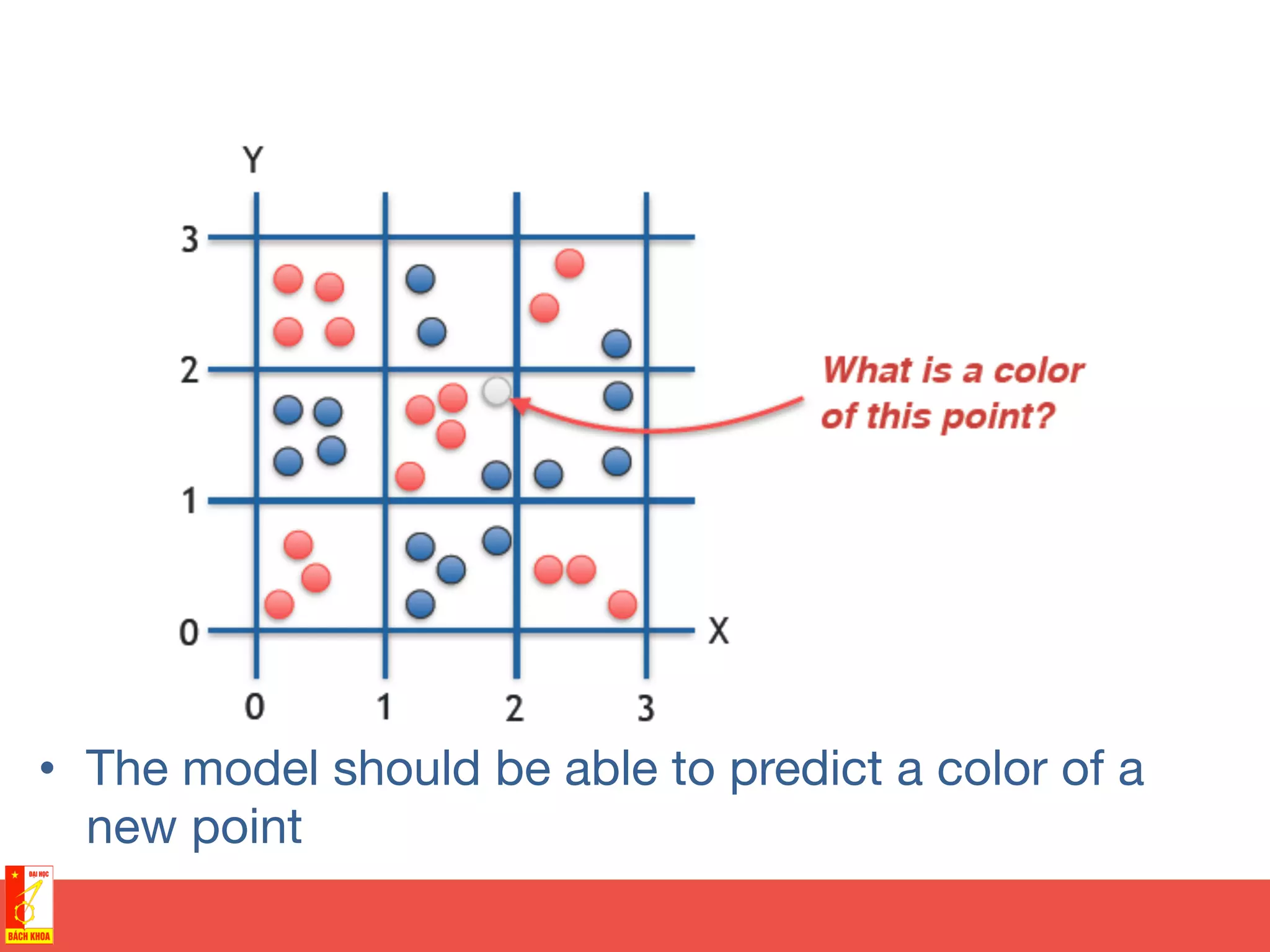
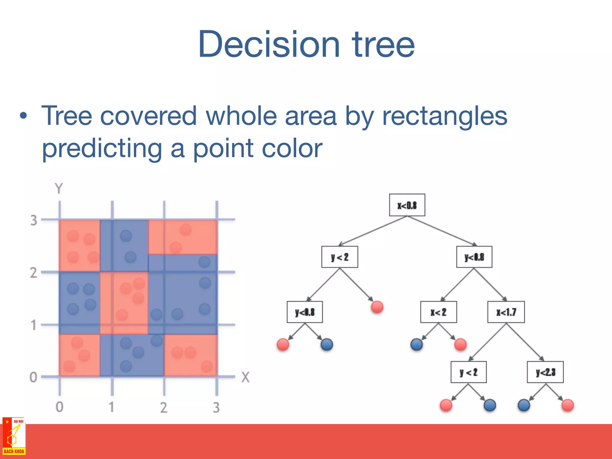
• Training sample of points
covering area [0,3] x [0,3]
• Two possible colors of
points](https://image.slidesharecdn.com/randomforests-150902071011-lva1-app6891/75/From-decision-trees-to-random-forests-35-2048.jpg)


![Motivation
• Training sample of points
covering area [0,3] x [0,3]
• Two possible colors of
points](https://crownmelresort.com/image.slidesharecdn.com/randomforests-150902071011-lva1-app6891/75/From-decision-trees-to-random-forests-35-2048.jpg)


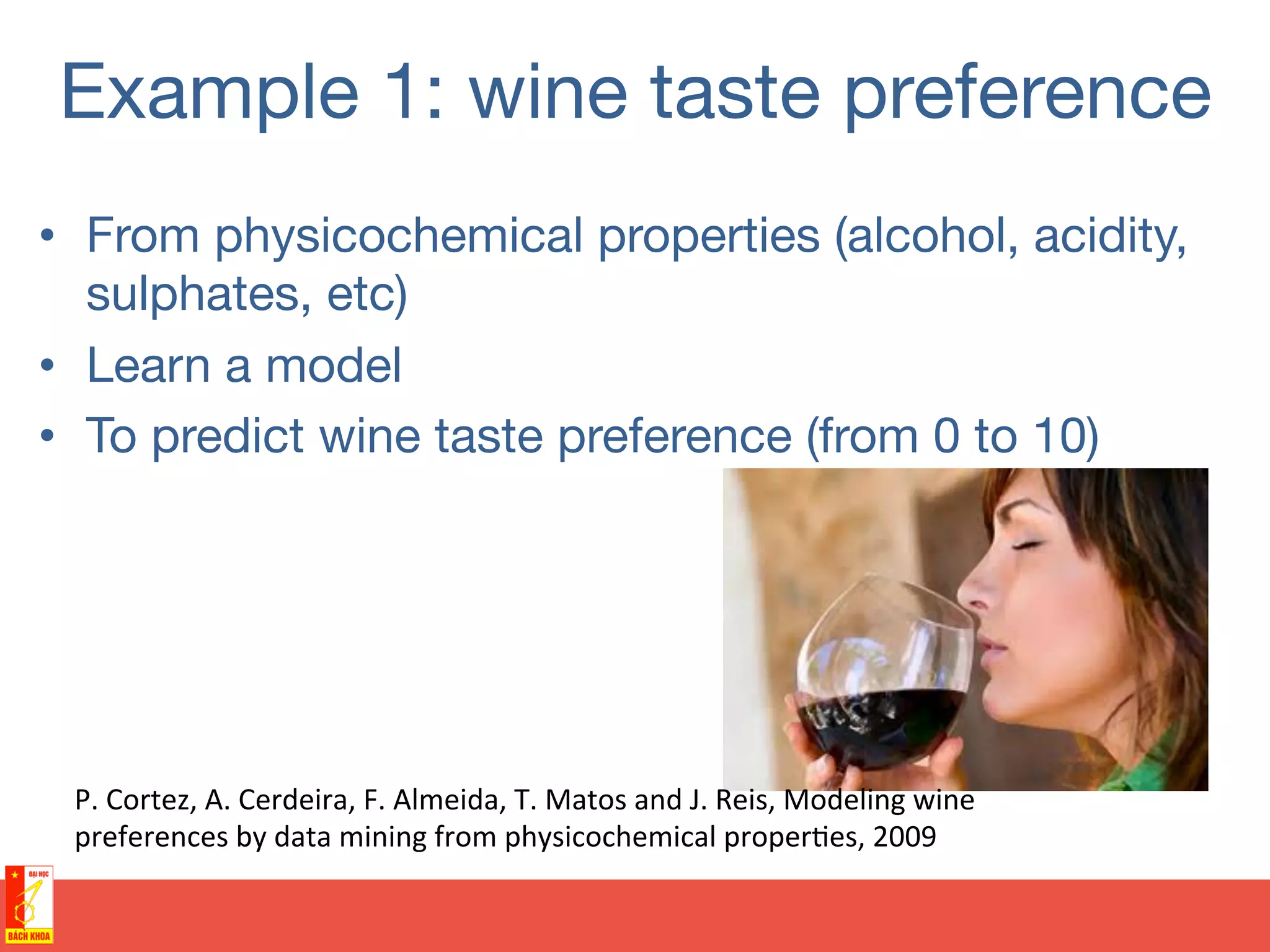
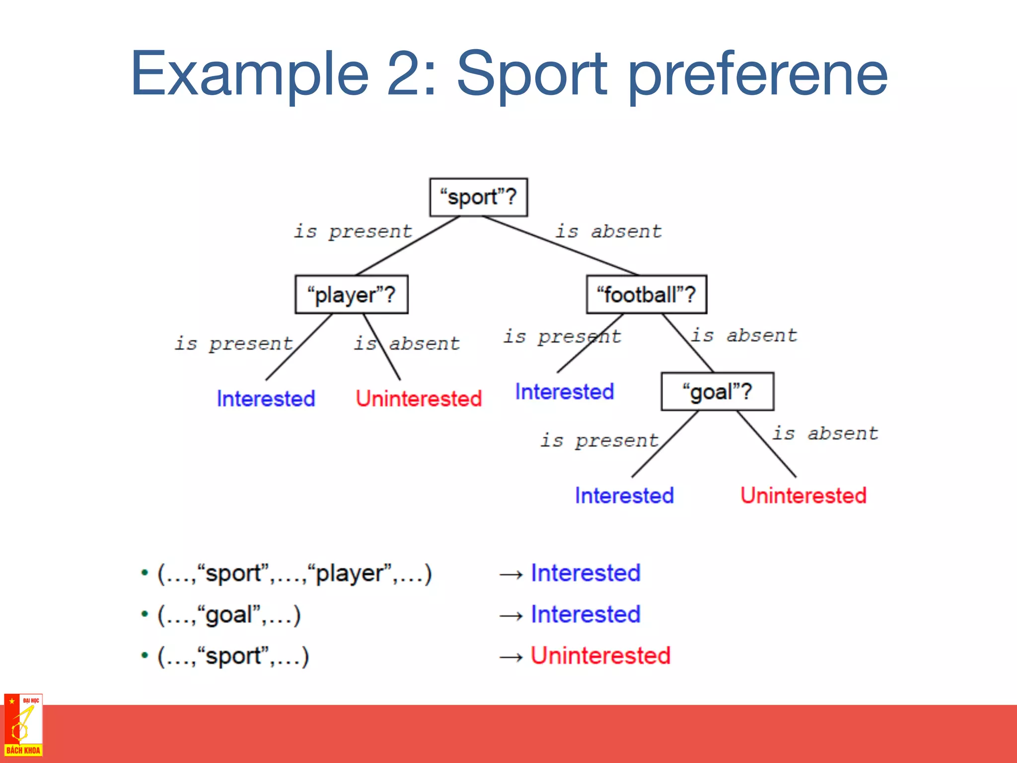
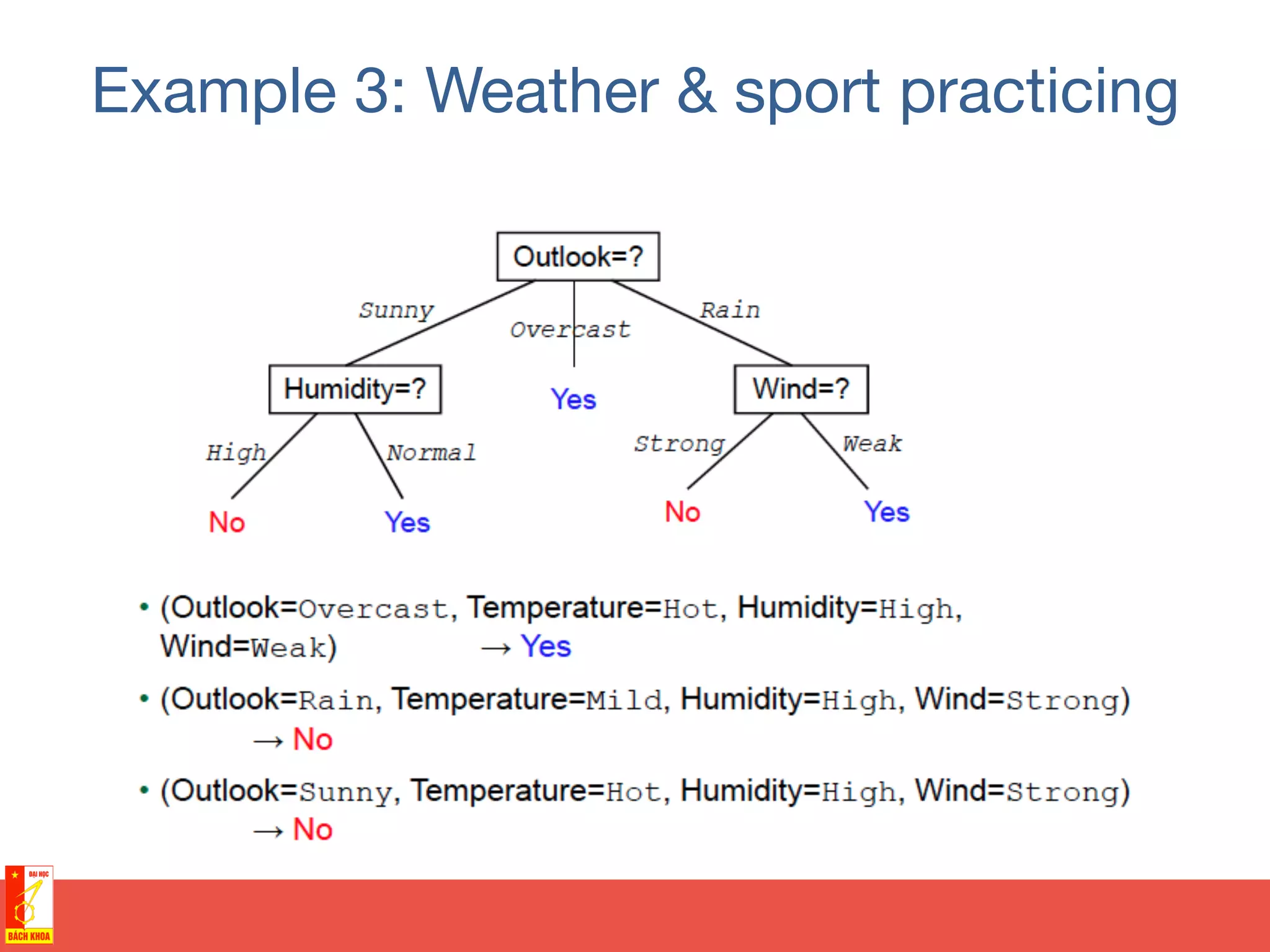
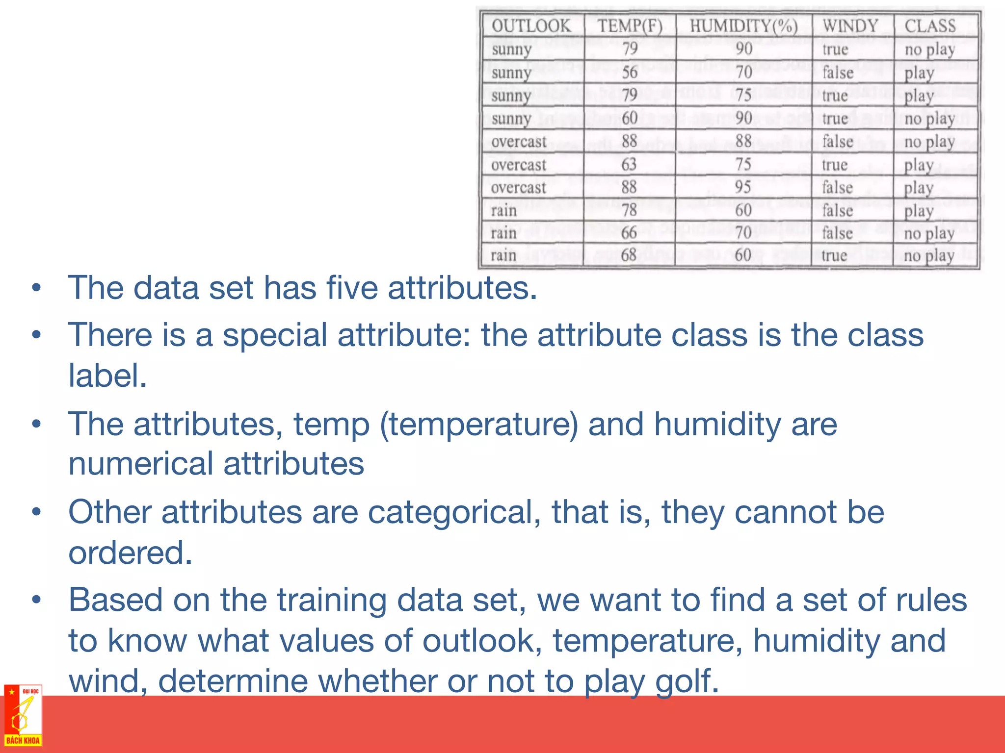
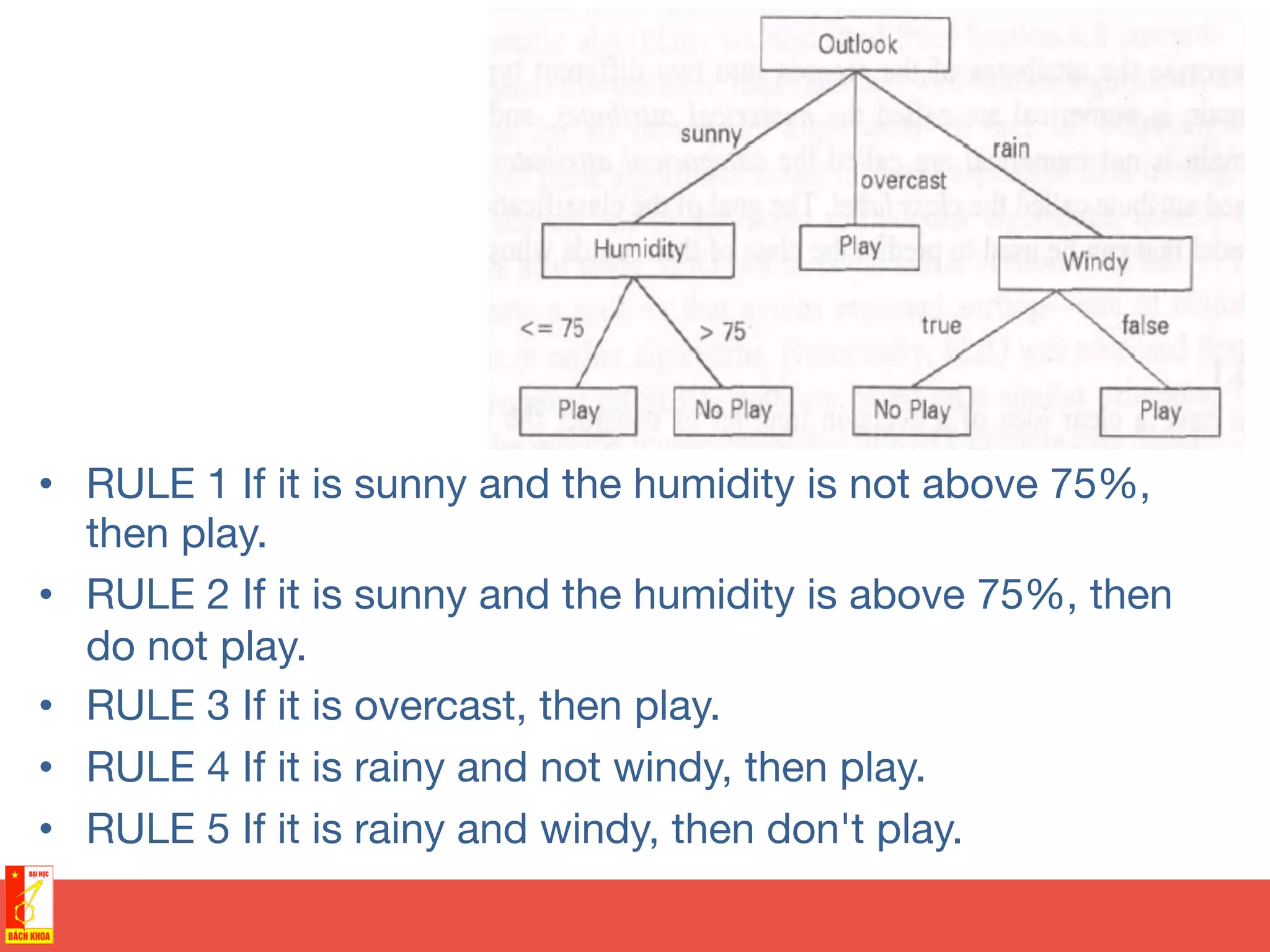
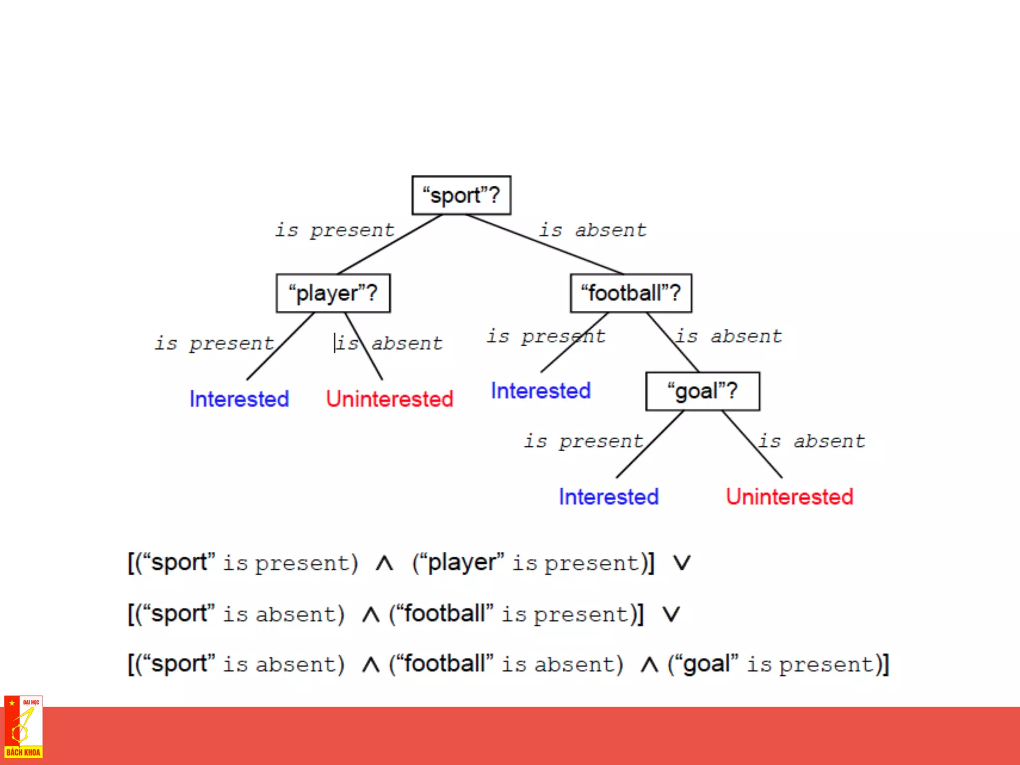
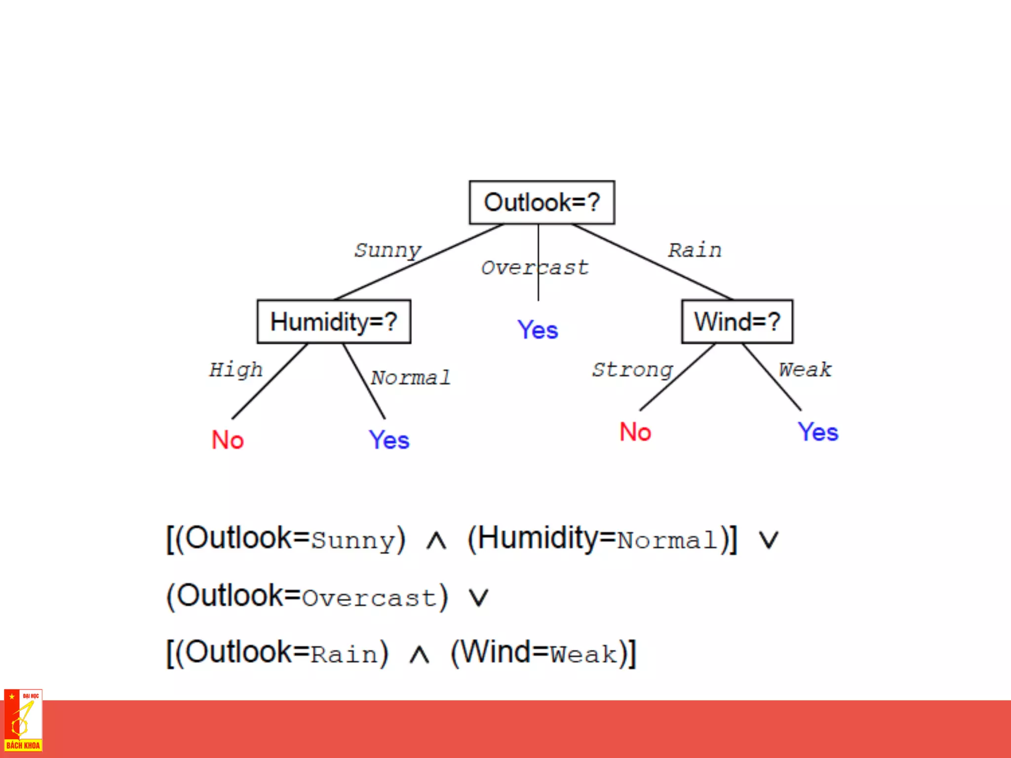
This document discusses decision trees and random forests for classification problems. It explains that decision trees use a top-down approach to split a training dataset based on attribute values to build a model for classification. Random forests improve upon decision trees by growing many de-correlated trees on randomly sampled subsets of data and features, then aggregating their predictions, which helps avoid overfitting. The document provides examples of using decision trees to classify wine preferences, sports preferences, and weather conditions for sport activities based on attribute values.