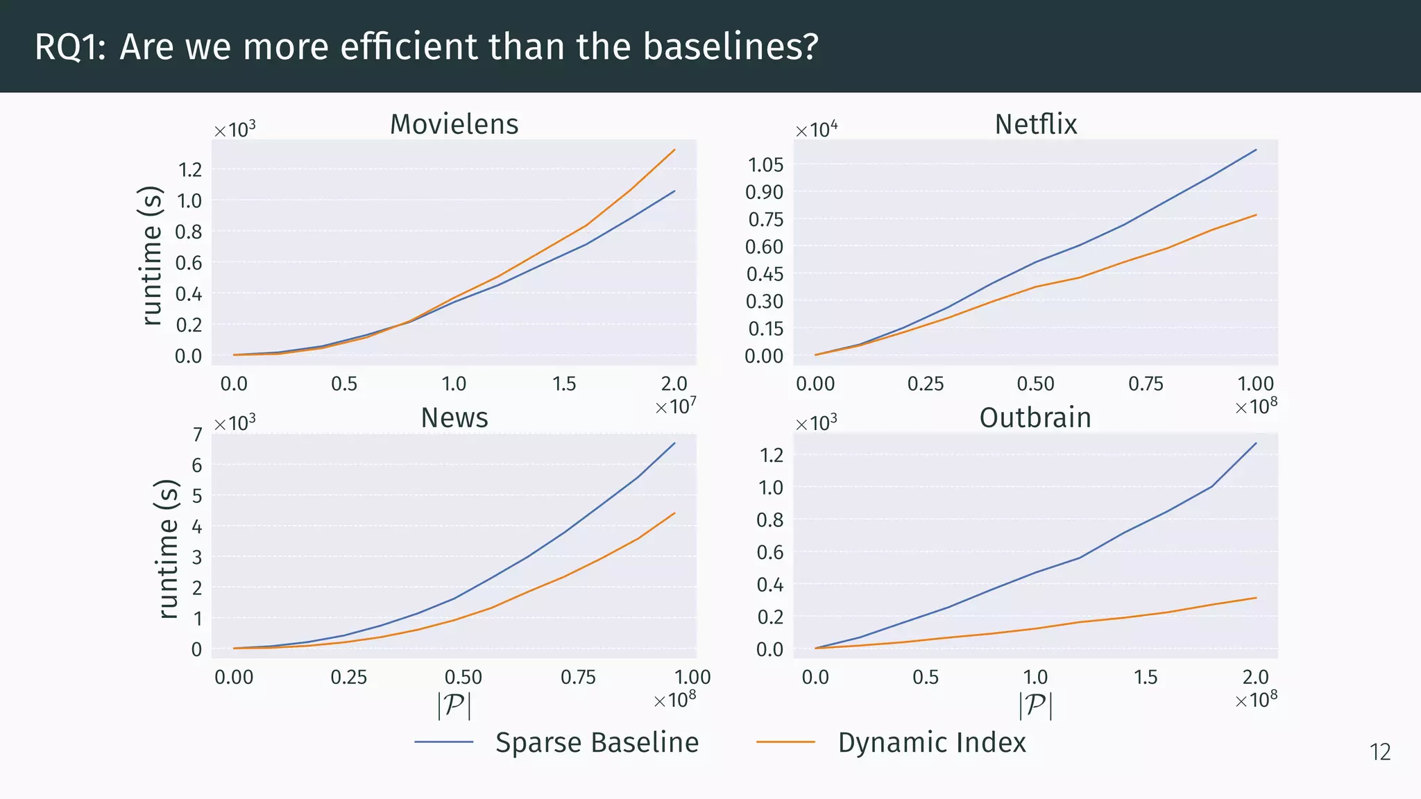
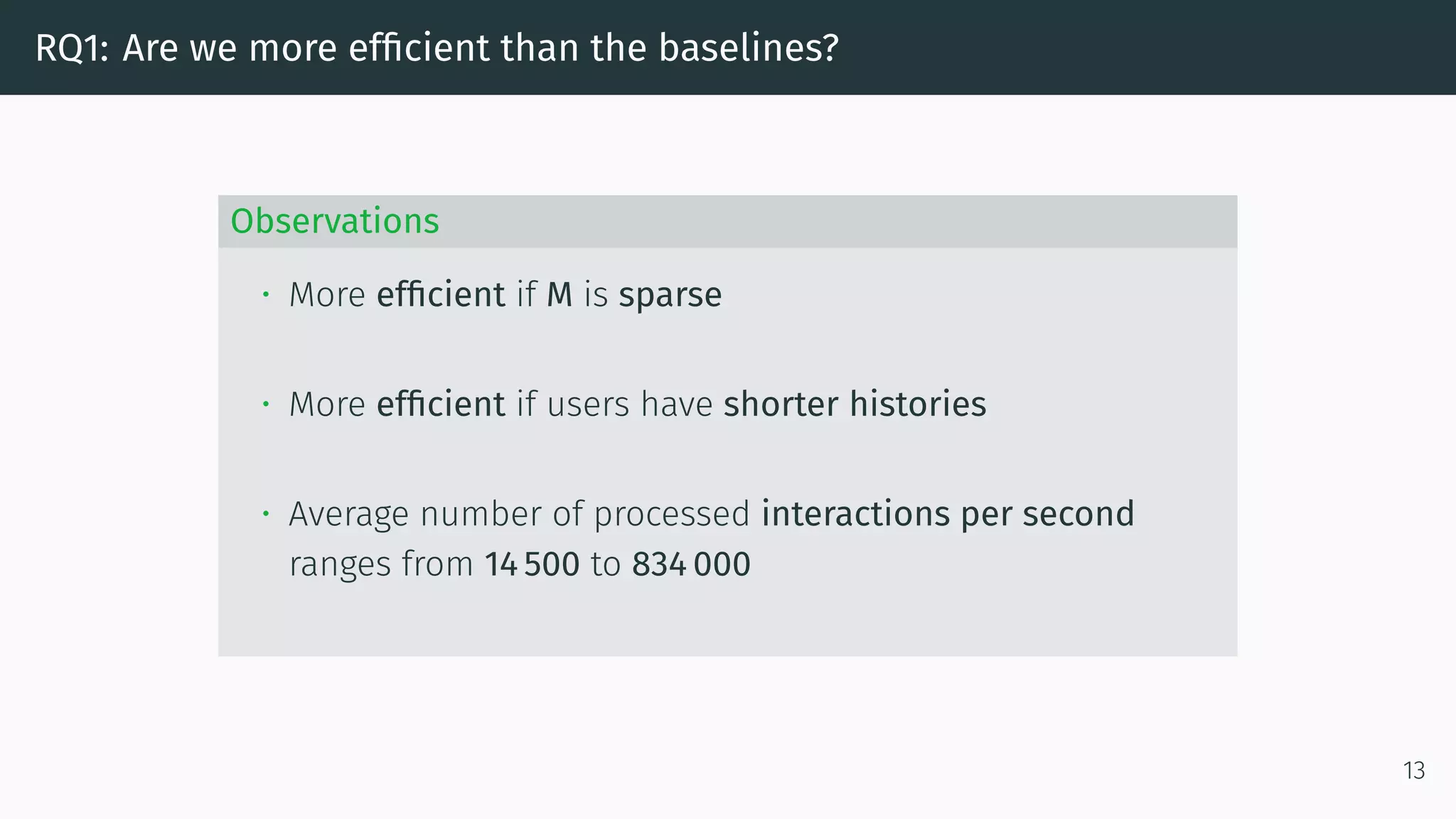
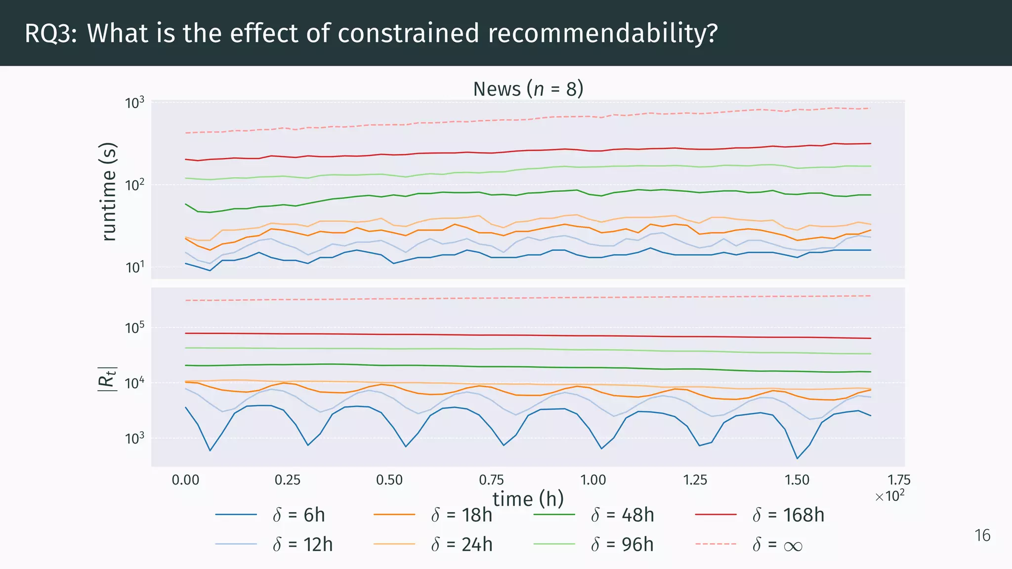
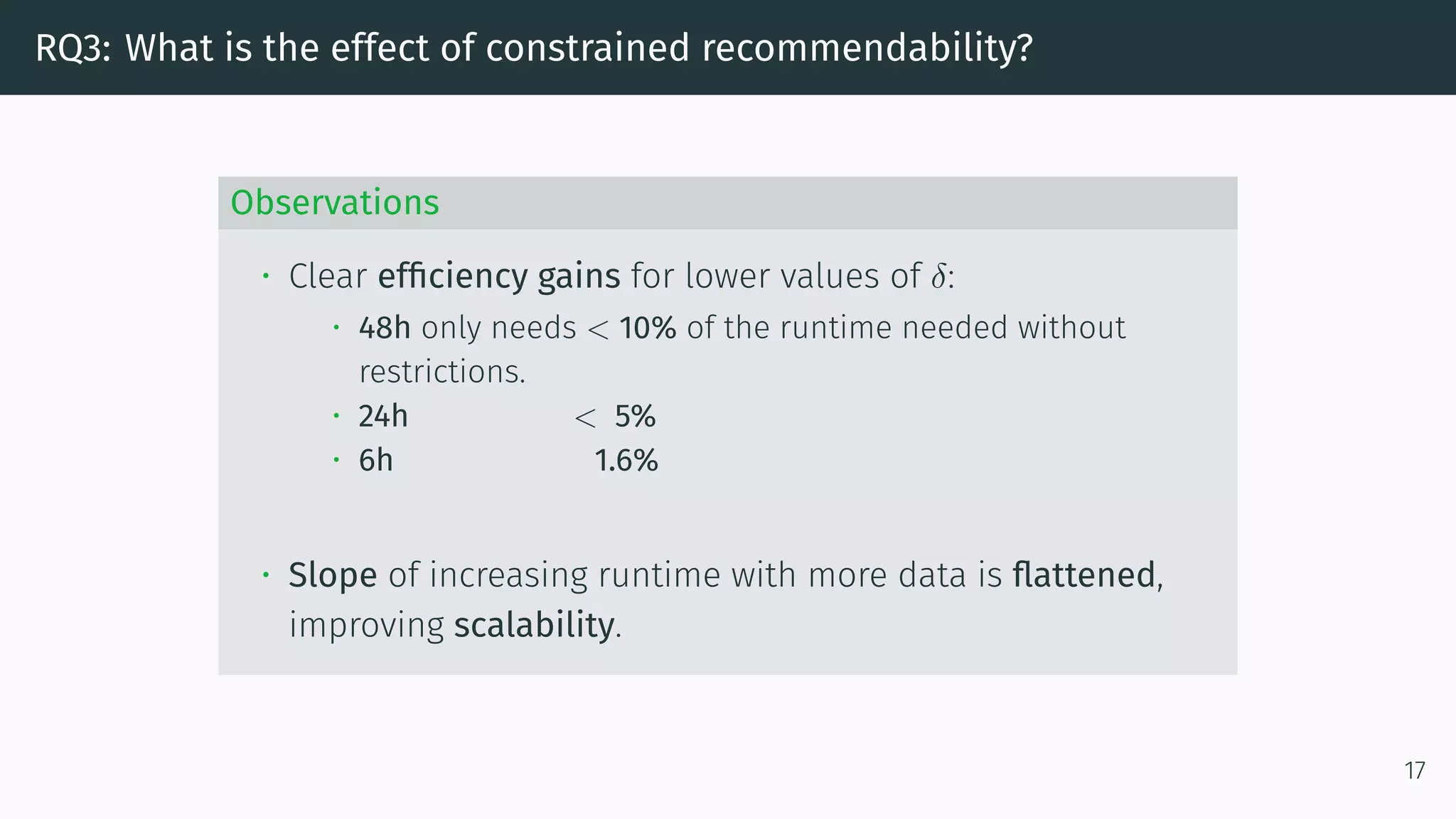
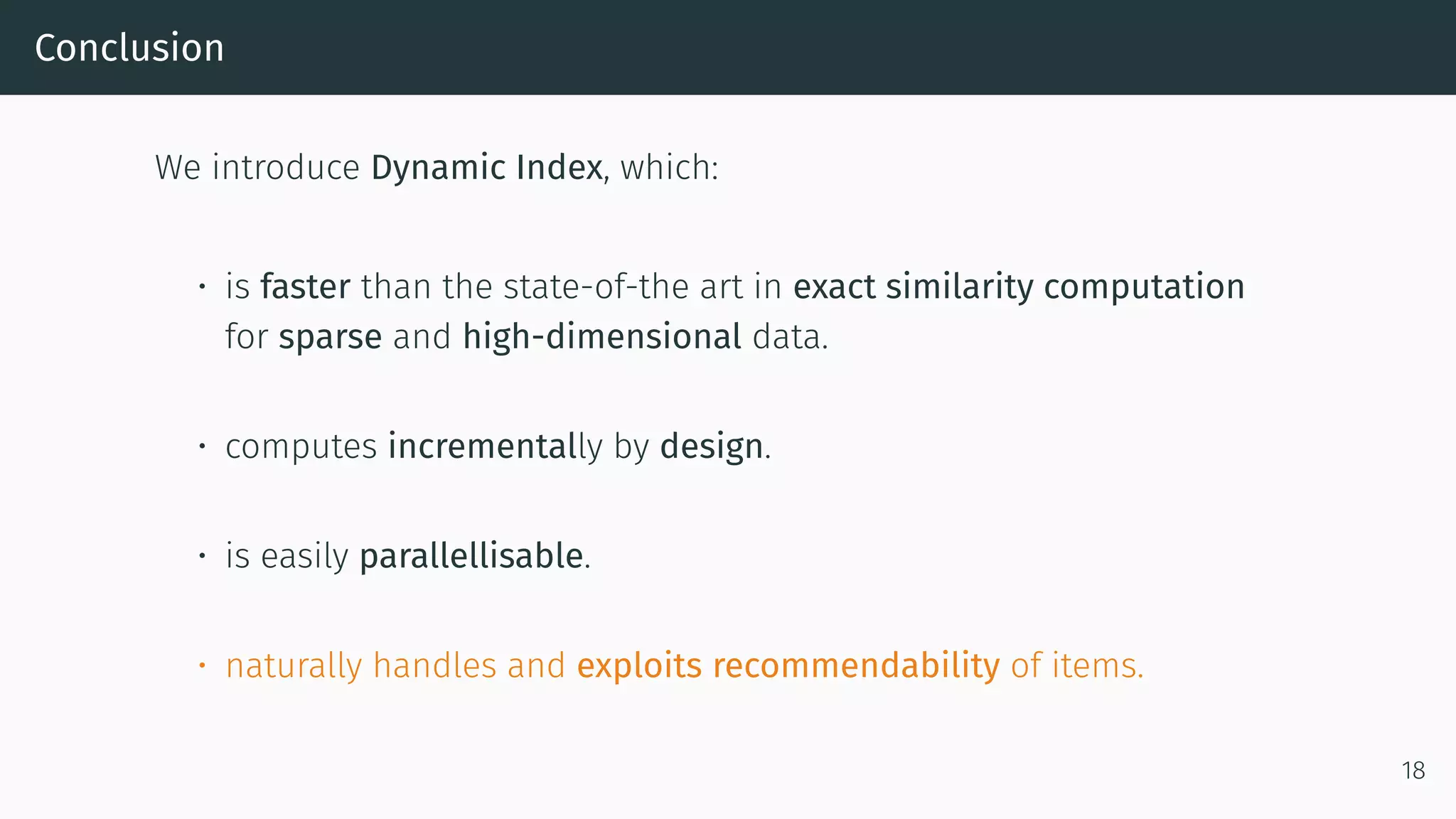
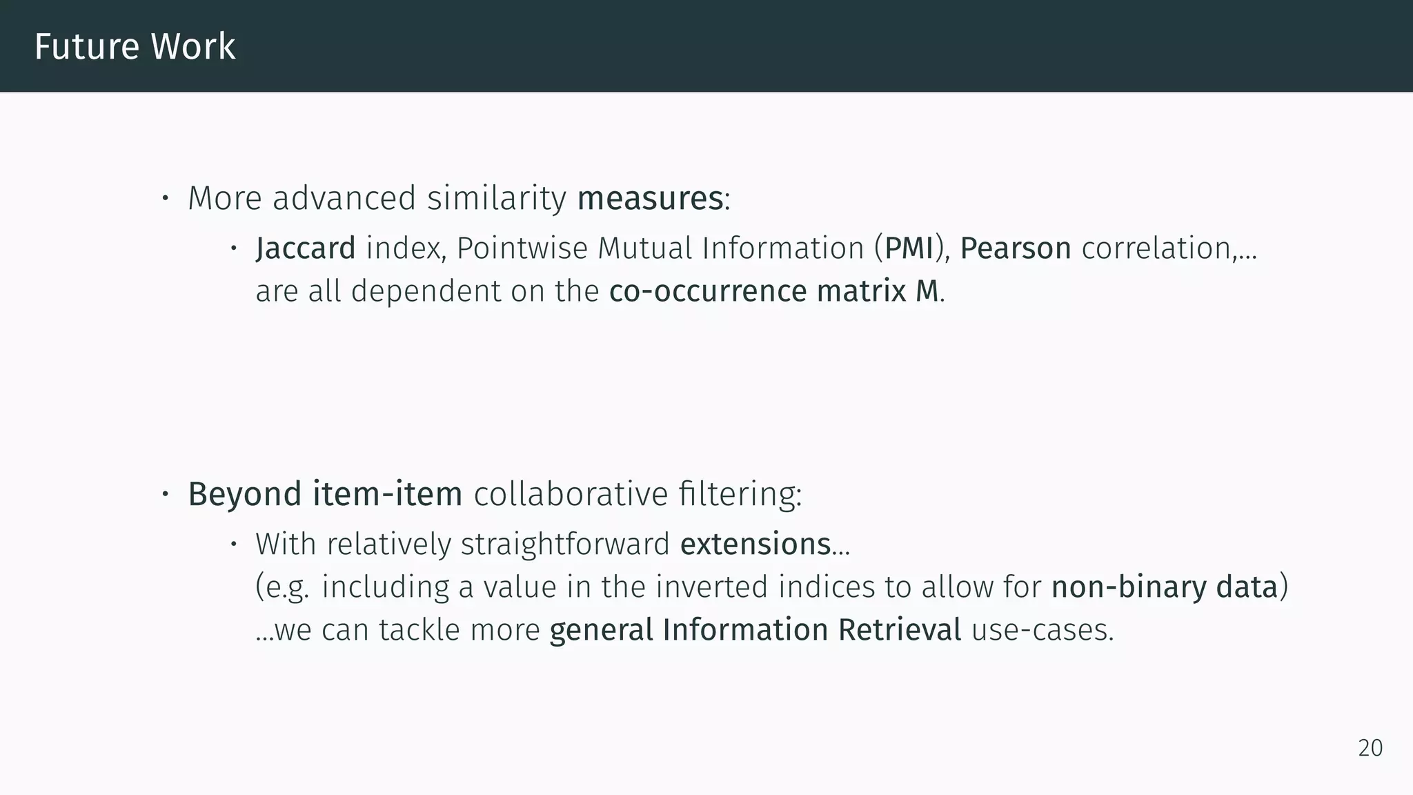
This document proposes a new method called Dynamic Index for efficiently computing similarity between items in collaborative filtering recommendations. It computes item similarities incrementally as user-item interactions stream in, by maintaining counts of co-occurrences between items and individual item exposures. This approach is faster than baselines for sparse datasets and scales to large data volumes. Parallelizing the method yields further speedups. Additionally, restricting recommendations to a subset of recent items significantly improves efficiency without harming recommendation quality.


![Parallellisation Procedure
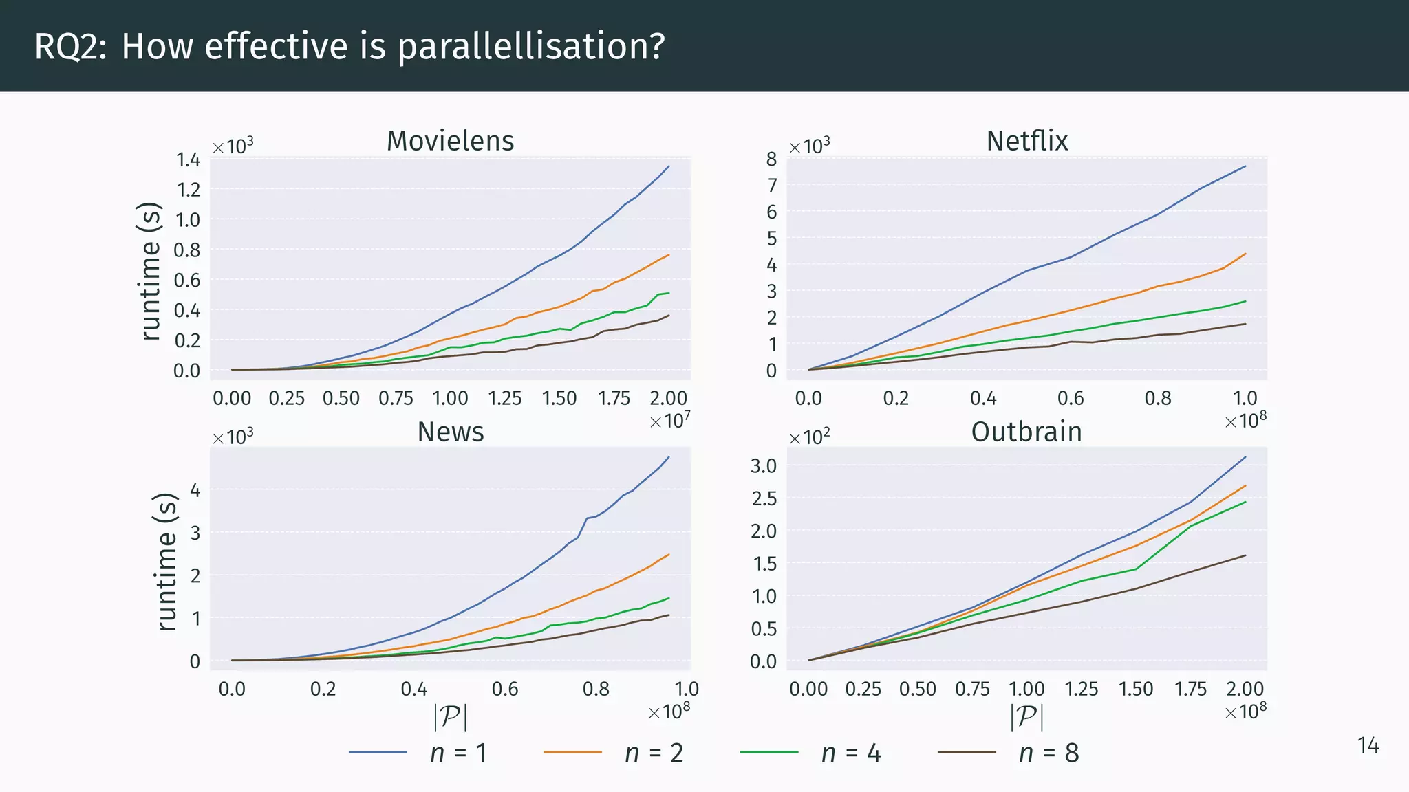
We adopt a MapReduce-like parallellisation framework:
• Mapping is the Dynamic Index algorithm.
• Reducing two models M = {M, N, L} and M = {M , N , L } is:
1. Summing up M, M and N, N
2. Cross-referencing (u, i)-pairs from L[u] with (u, j)-pairs from L [u].
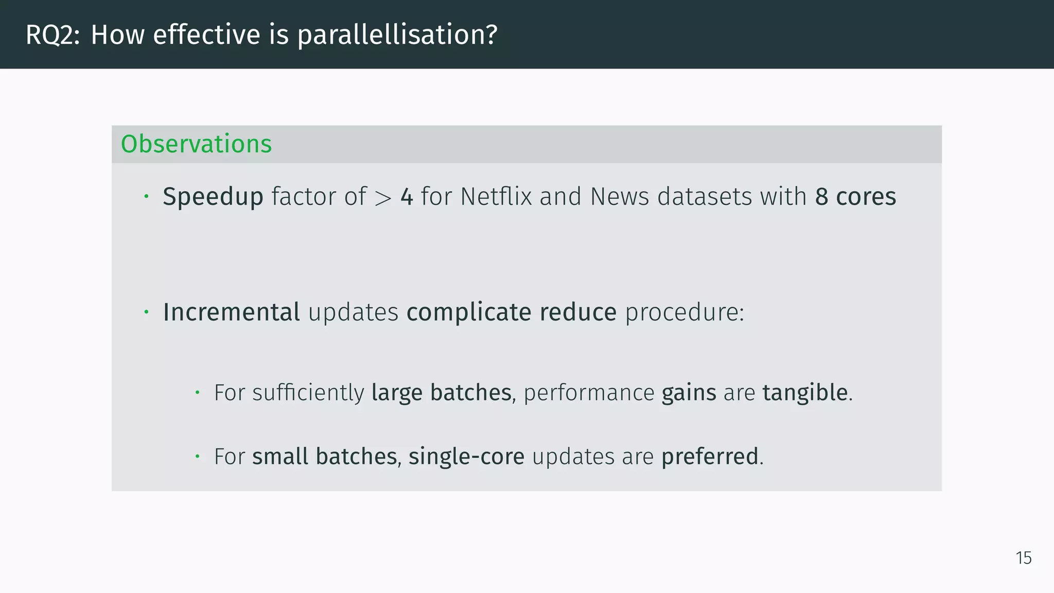
Step 2 is obsolete if M and M are computed on disjoint sets of users!
9](https://image.slidesharecdn.com/finalpresentationrecsys-190926161411/75/Efficient-Similarity-Computation-for-Collaborative-Filtering-in-Dynamic-Environments-ACM-RecSys-2019-11-2048.jpg)


![Parallellisation Procedure
We adopt a MapReduce-like parallellisation framework:
• Mapping is the Dynamic Index algorithm.
• Reducing two models M = {M, N, L} and M = {M , N , L } is:
1. Summing up M, M and N, N
2. Cross-referencing (u, i)-pairs from L[u] with (u, j)-pairs from L [u].
Step 2 is obsolete if M and M are computed on disjoint sets of users!
9](https://crownmelresort.com/image.slidesharecdn.com/finalpresentationrecsys-190926161411/75/Efficient-Similarity-Computation-for-Collaborative-Filtering-in-Dynamic-Environments-ACM-RecSys-2019-11-2048.jpg)


![[系列活動] 人工智慧與機器學習在推薦系統上的應用](https://cdn.slidesharecdn.com/ss_thumbnails/merged-161217165734-thumbnail.jpg?width=640&height=640&fit=bounds)


