Download as PDF, PPTX

![Data Mining Tasks
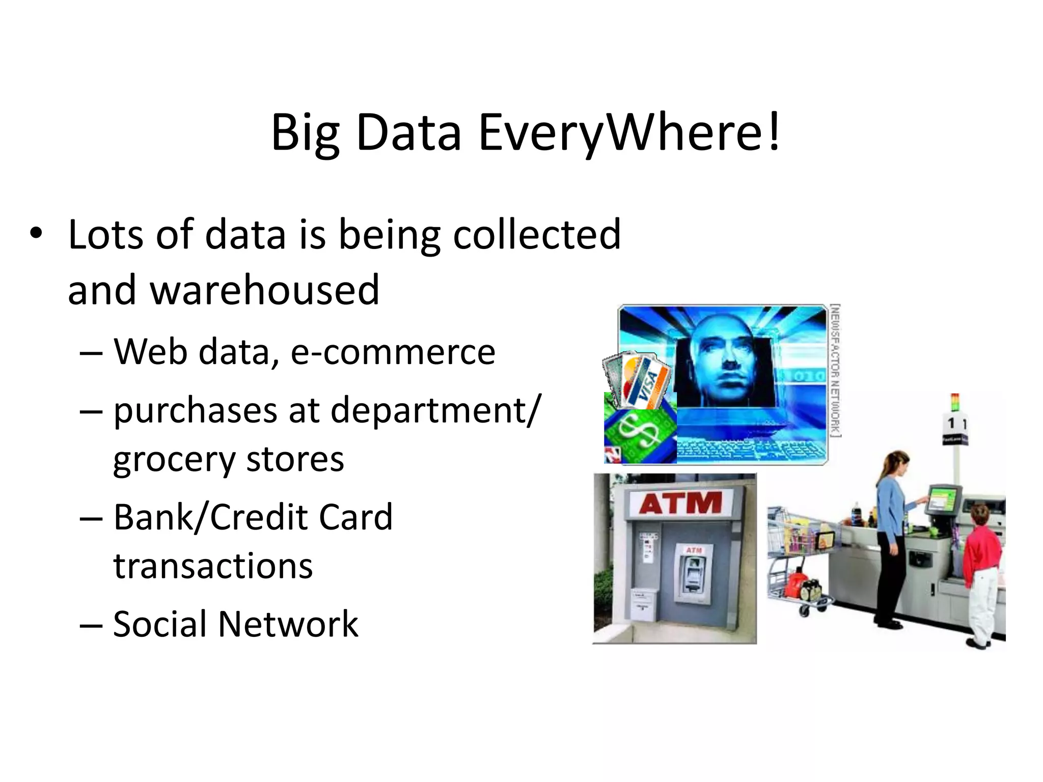
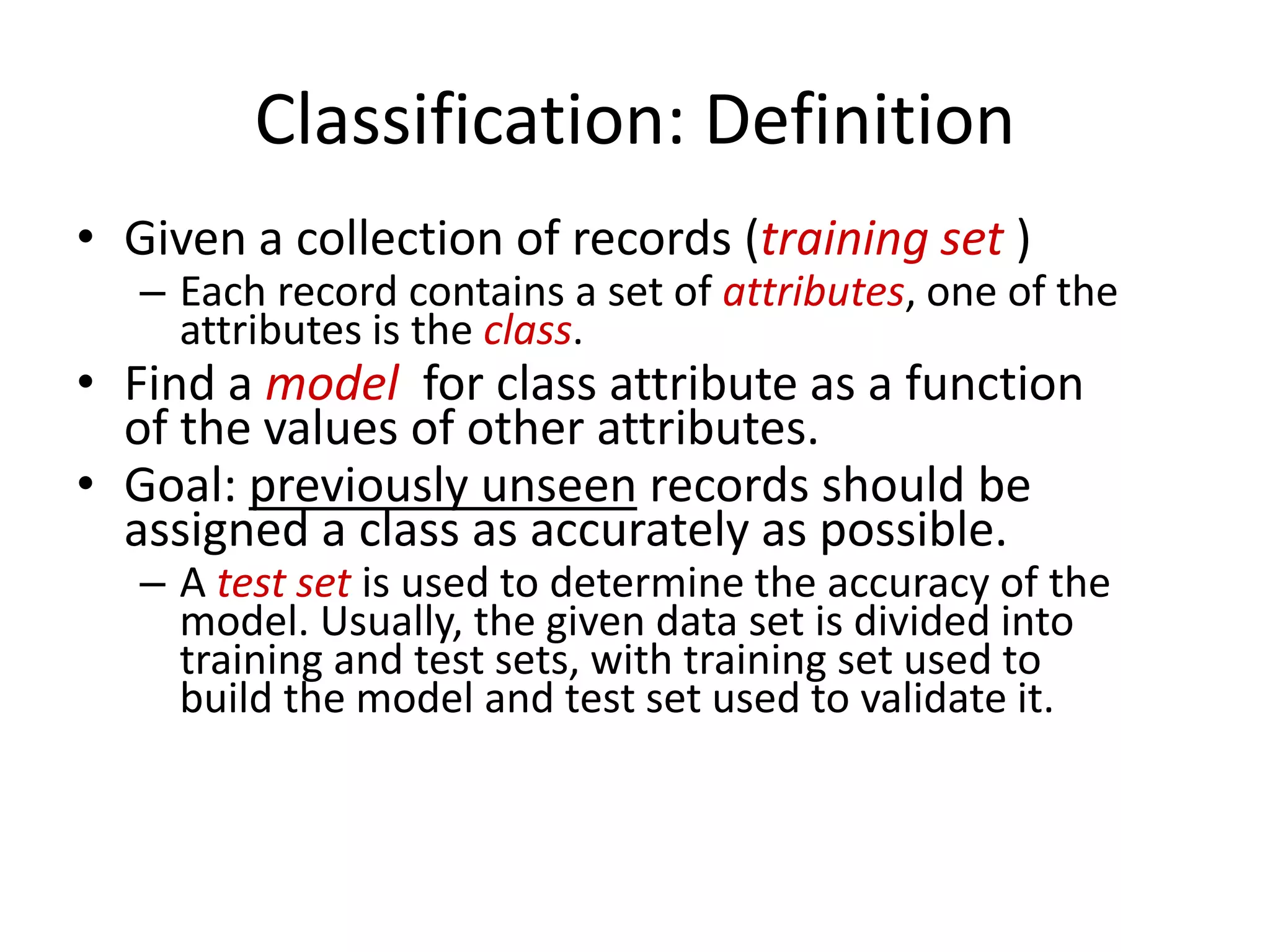
•Classification [Predictive]
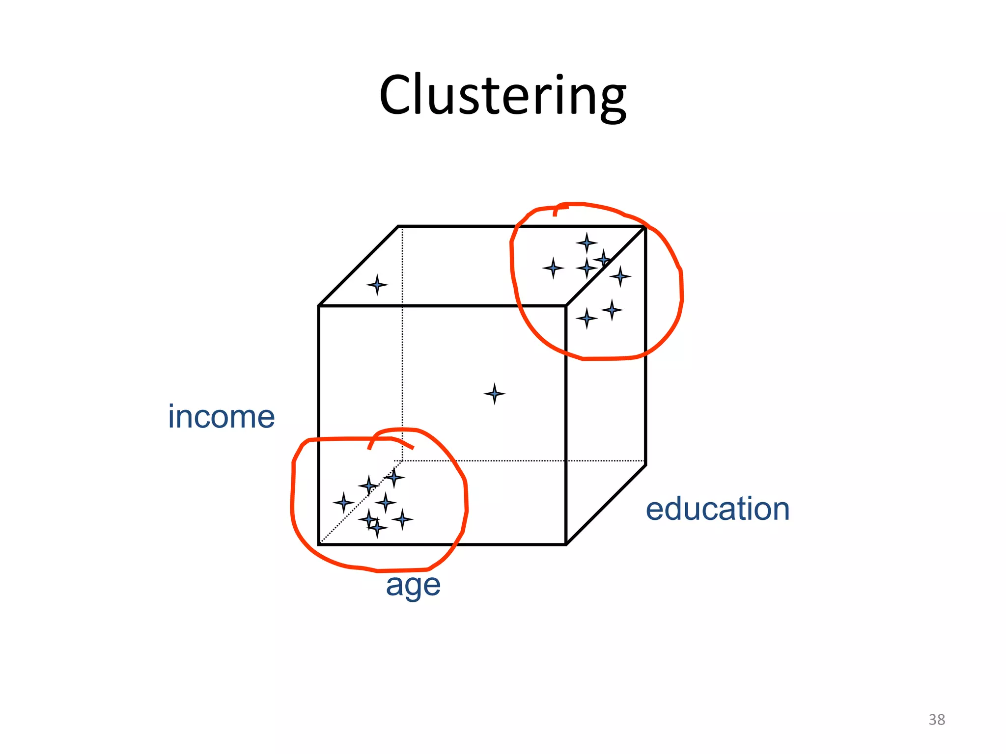
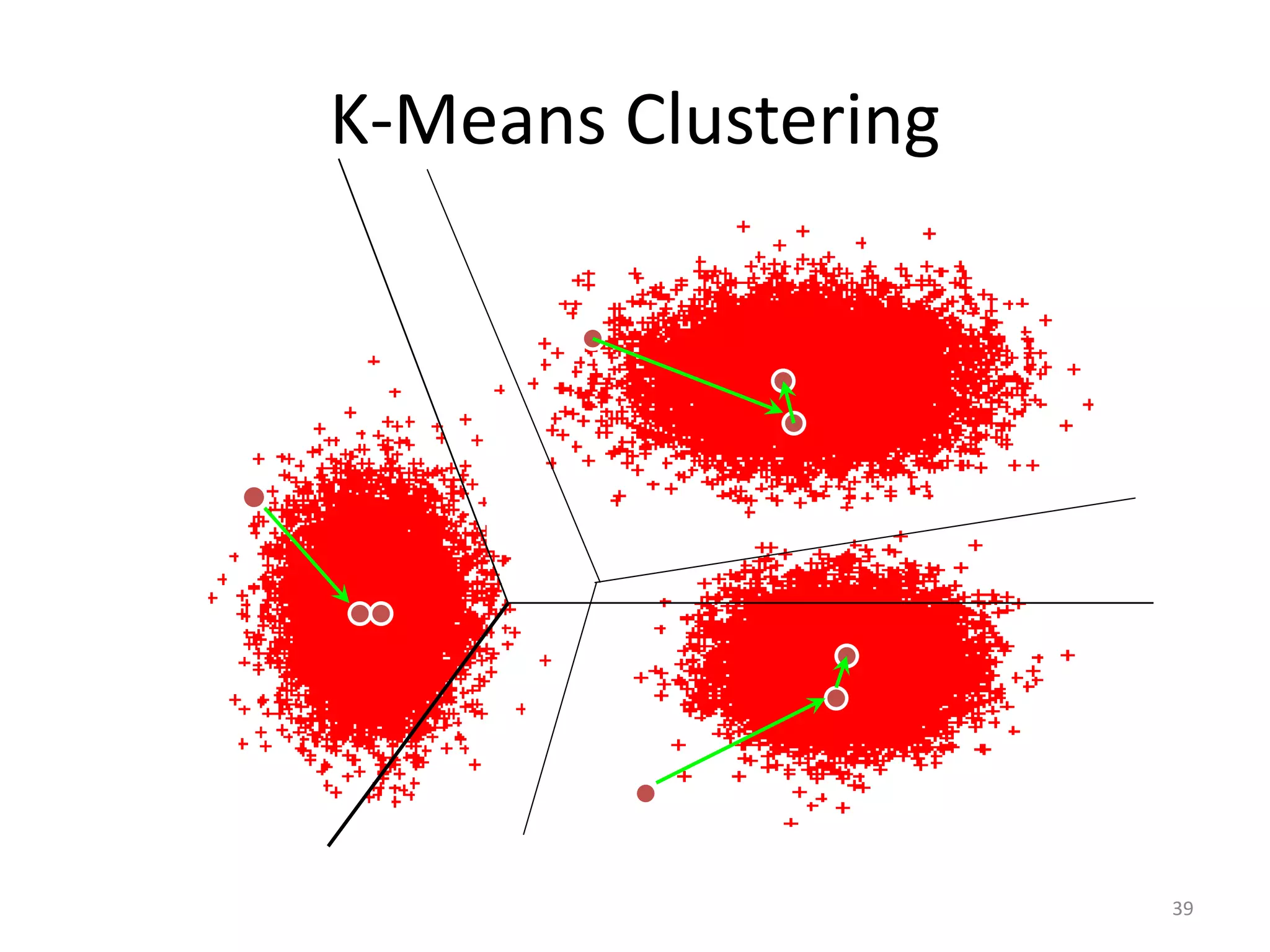
•Clustering [Descriptive]
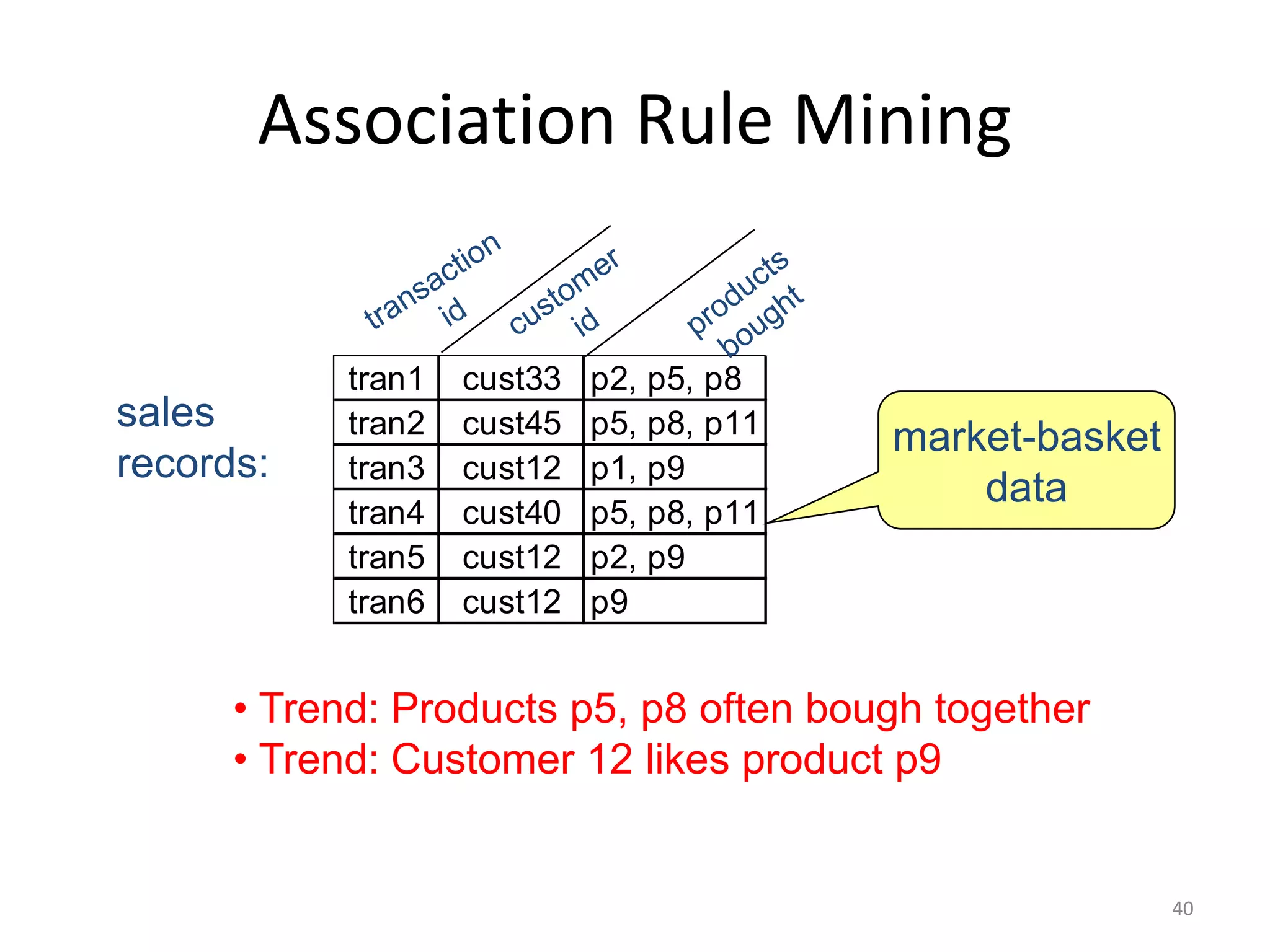
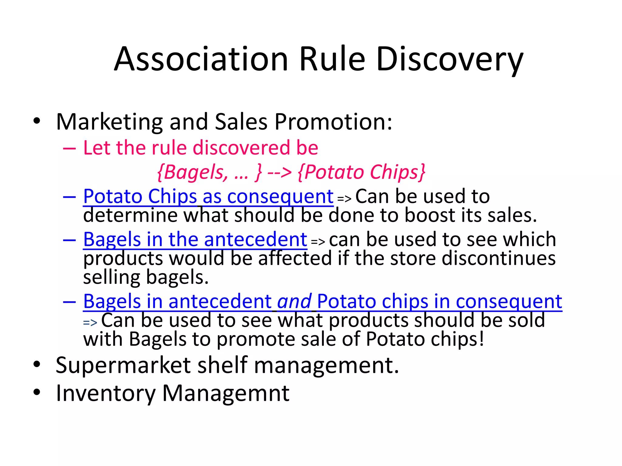
•Association Rule Discovery [Descriptive]
•Sequential Pattern Discovery [Descriptive]
•Regression [Predictive]
•Deviation Detection [Predictive]
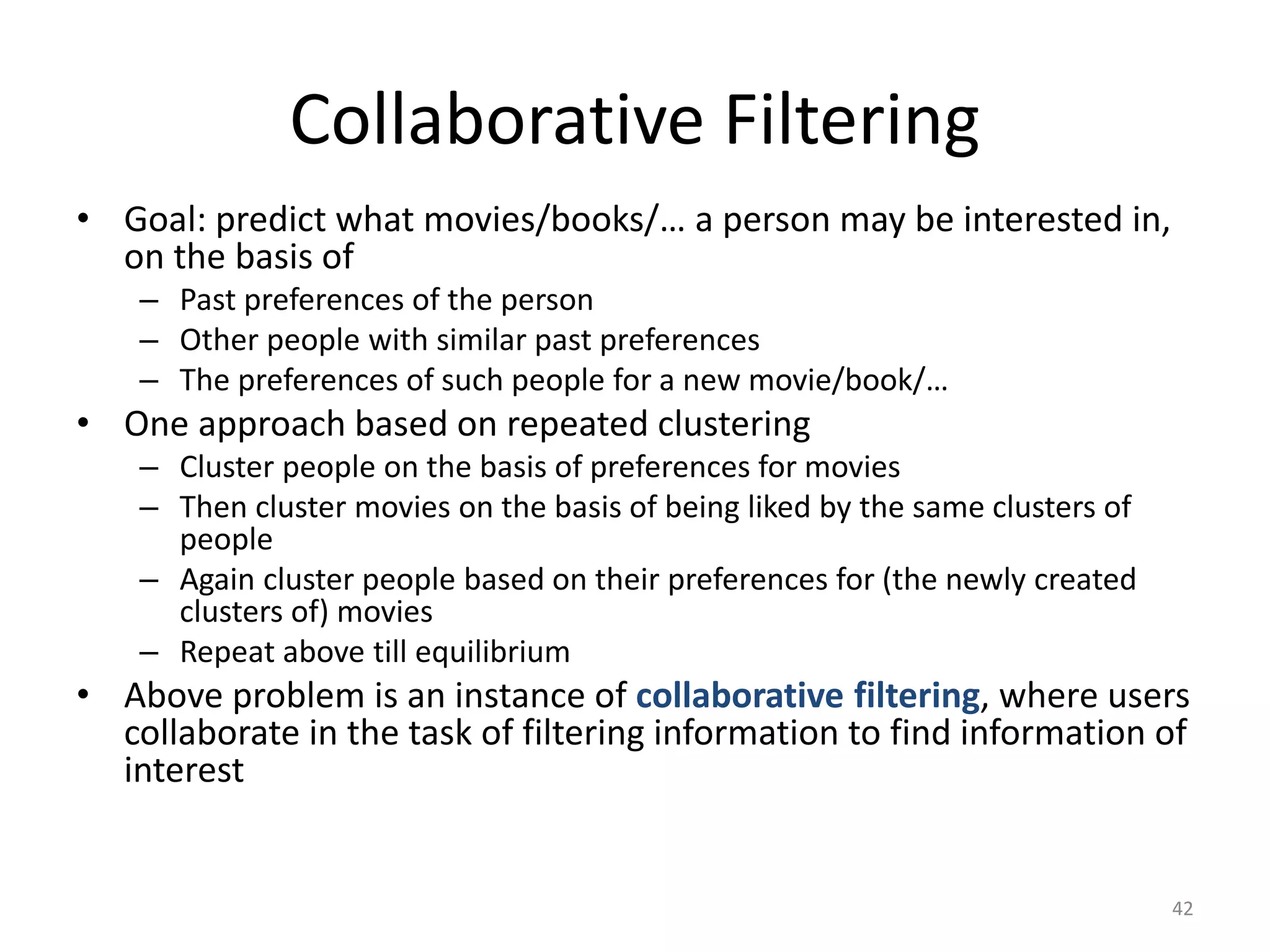
•Collaborative Filter [Predictive]](https://image.slidesharecdn.com/bigdata-141009021403-conversion-gate01/75/Big-data-35-2048.jpg)
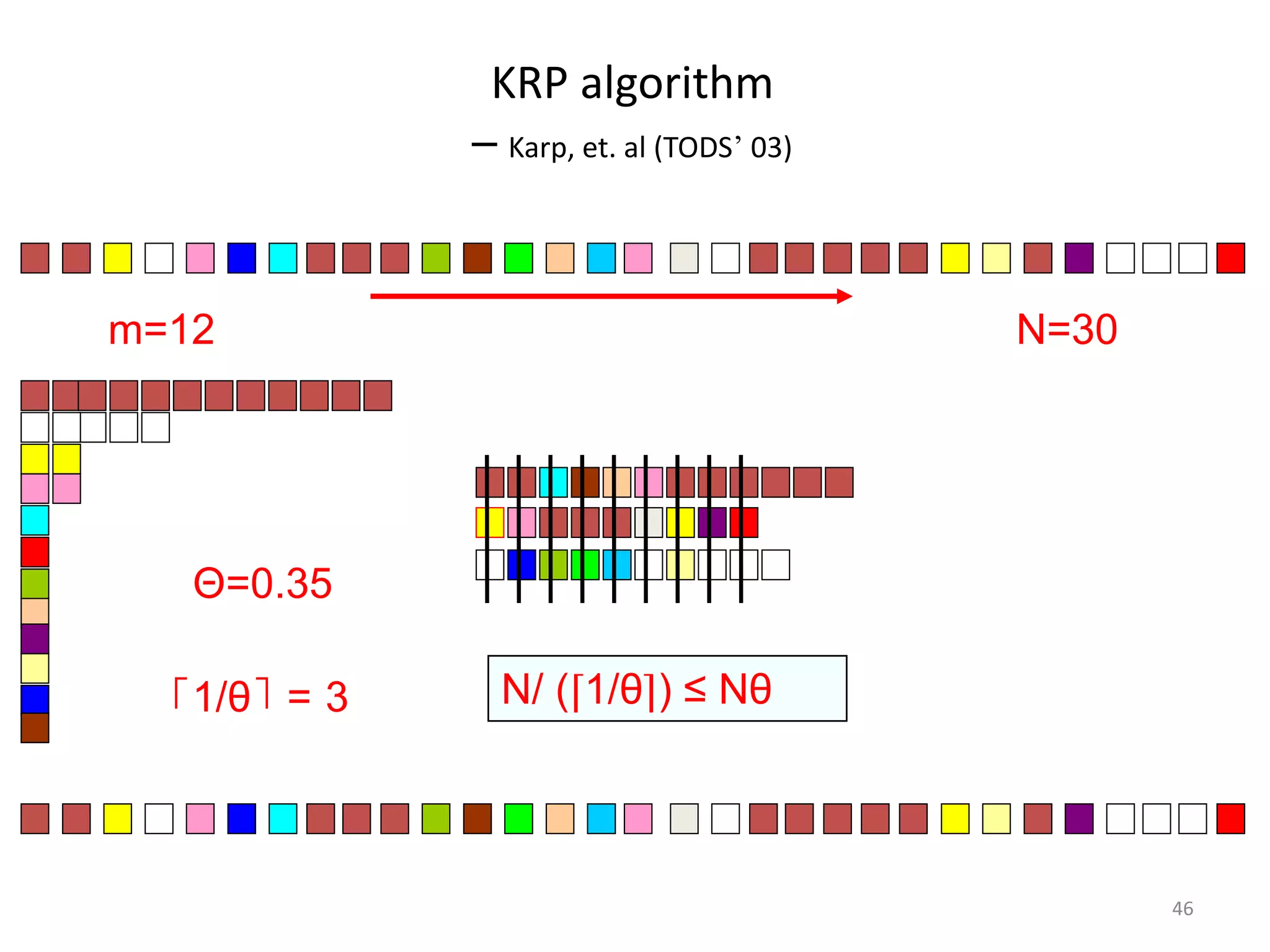
![A Simple Problem
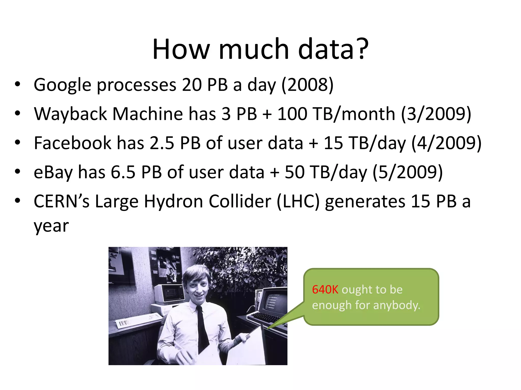
•Finding frequent items
–Given a sequence (x1,…xN) where xi∈[1,m], and a real number θbetween zero and one.
–Looking for xiwhose frequency > θ
–Naïve Algorithm (m counters)
•The number of frequent items ≤ 1/θ
•Problem: N>>m>>1/θ
45
P×(Nθ) ≤ N](https://image.slidesharecdn.com/bigdata-141009021403-conversion-gate01/75/Big-data-45-2048.jpg)


![Data Mining Tasks
•Classification [Predictive]
•Clustering [Descriptive]
•Association Rule Discovery [Descriptive]
•Sequential Pattern Discovery [Descriptive]
•Regression [Predictive]
•Deviation Detection [Predictive]
•Collaborative Filter [Predictive]](https://crownmelresort.com/image.slidesharecdn.com/bigdata-141009021403-conversion-gate01/75/Big-data-35-2048.jpg)


![A Simple Problem
•Finding frequent items
–Given a sequence (x1,…xN) where xi∈[1,m], and a real number θbetween zero and one.
–Looking for xiwhose frequency > θ
–Naïve Algorithm (m counters)
•The number of frequent items ≤ 1/θ
•Problem: N>>m>>1/θ
45
P×(Nθ) ≤ N](https://crownmelresort.com/image.slidesharecdn.com/bigdata-141009021403-conversion-gate01/75/Big-data-45-2048.jpg)


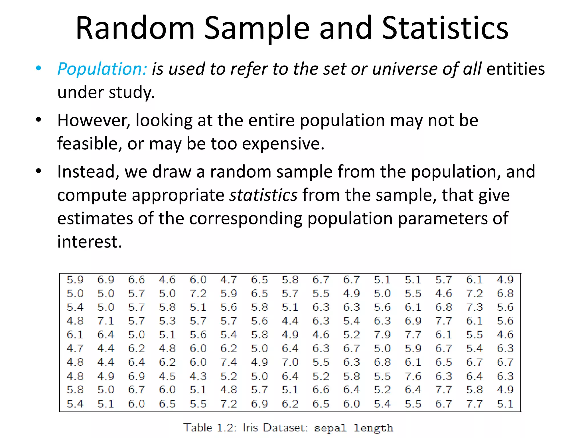
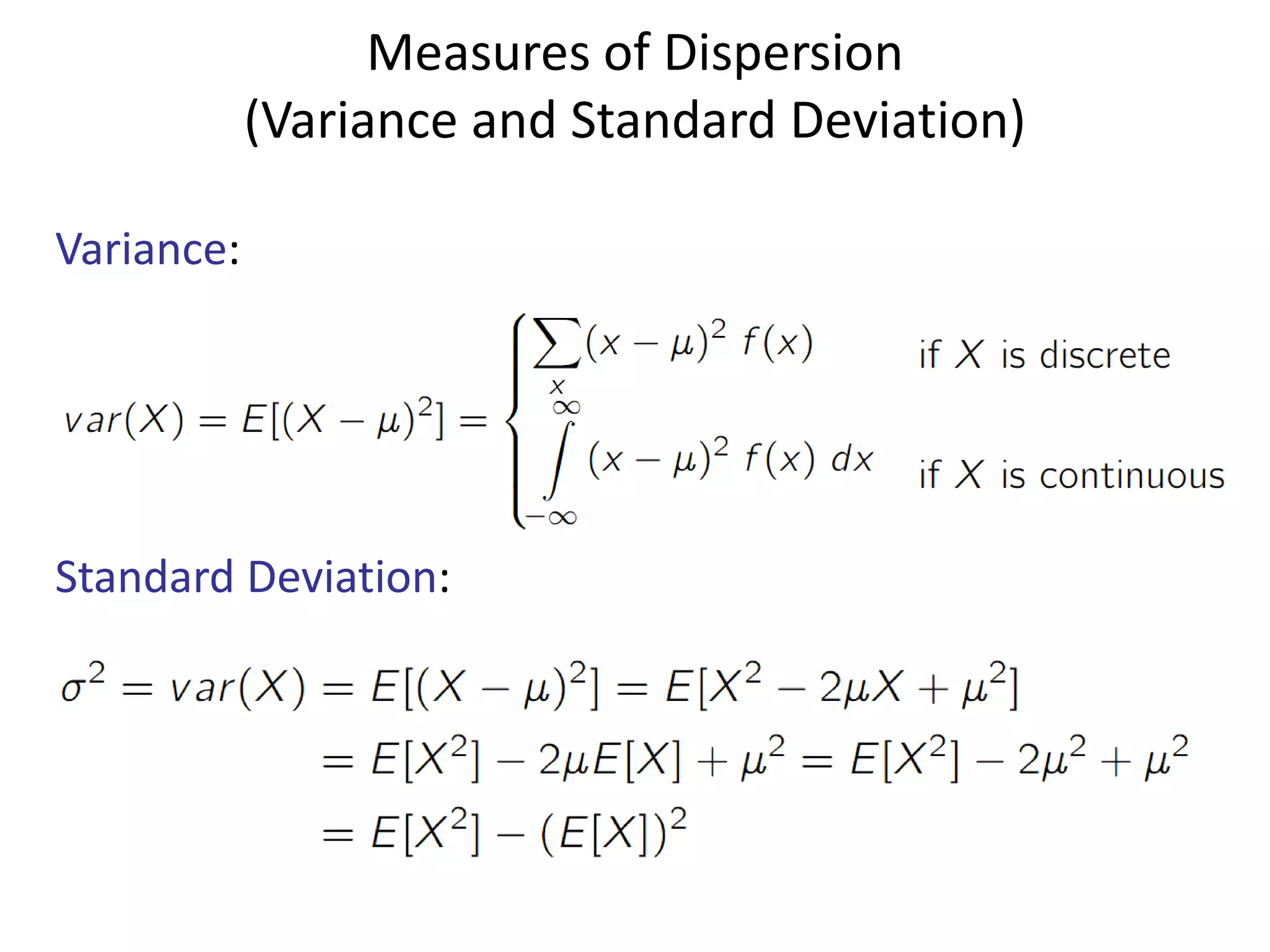
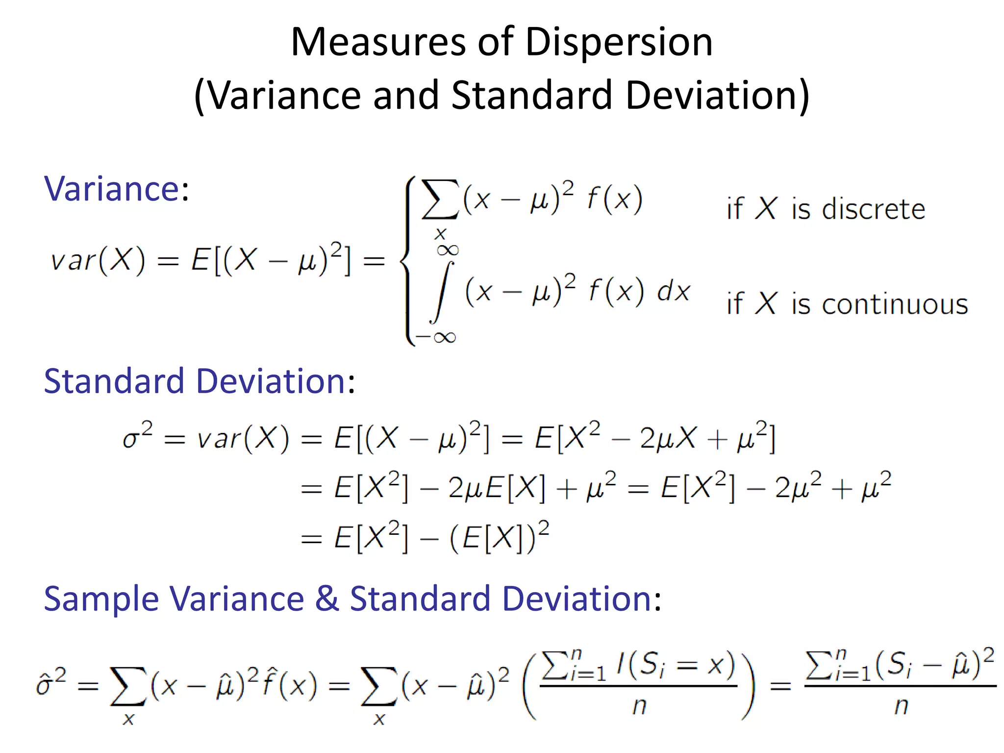
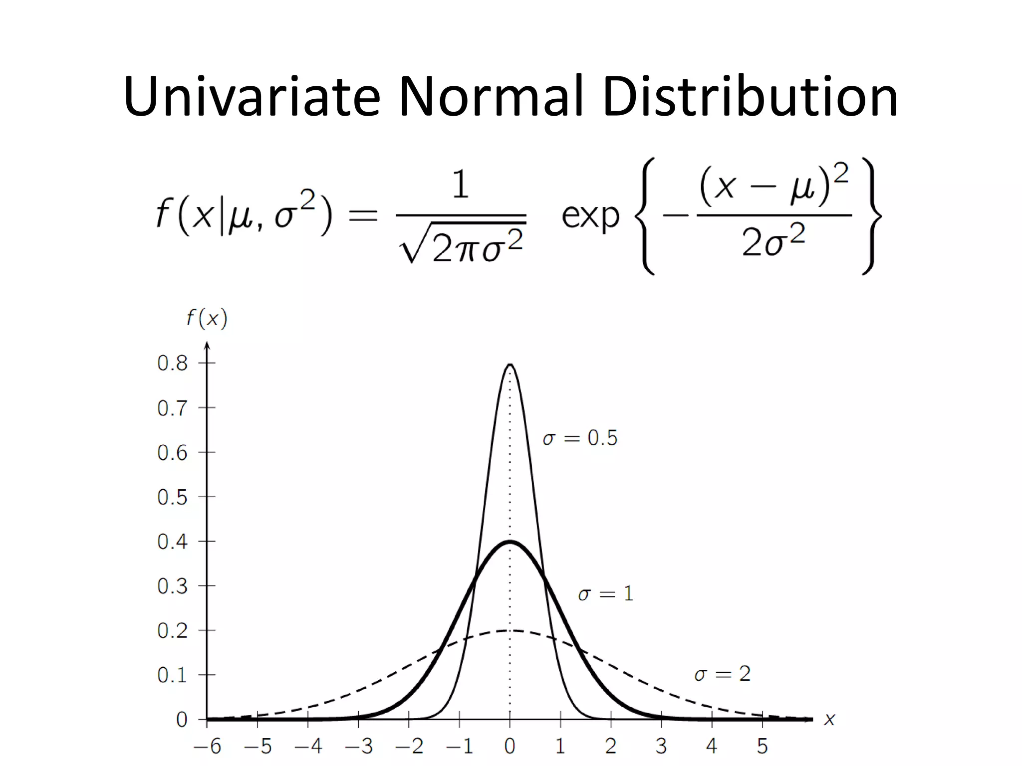
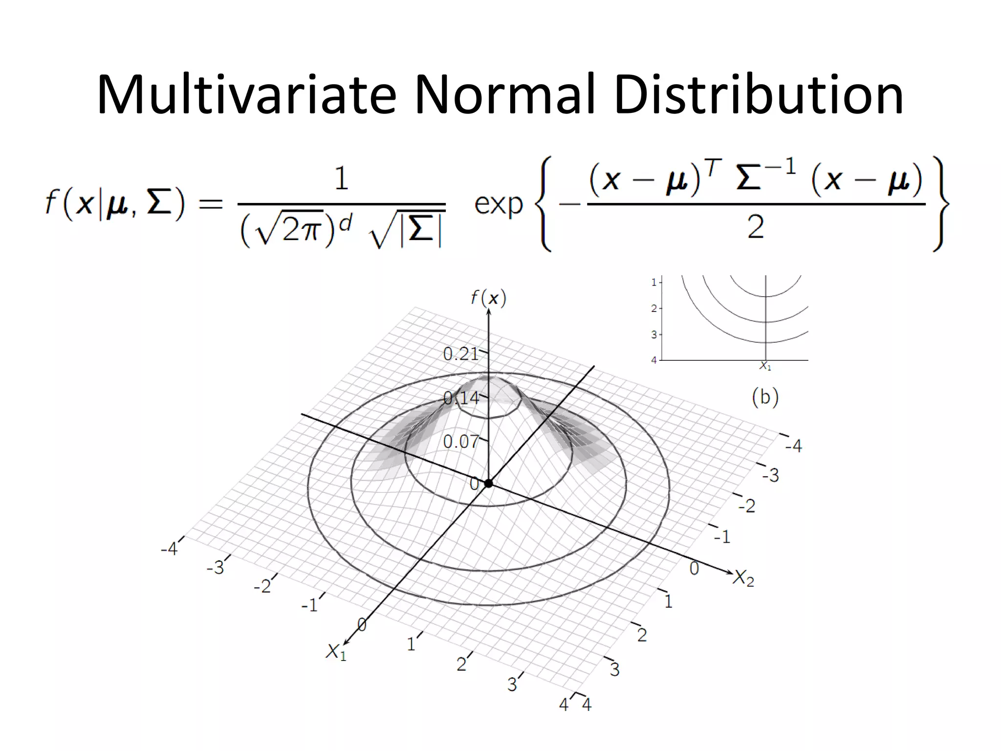
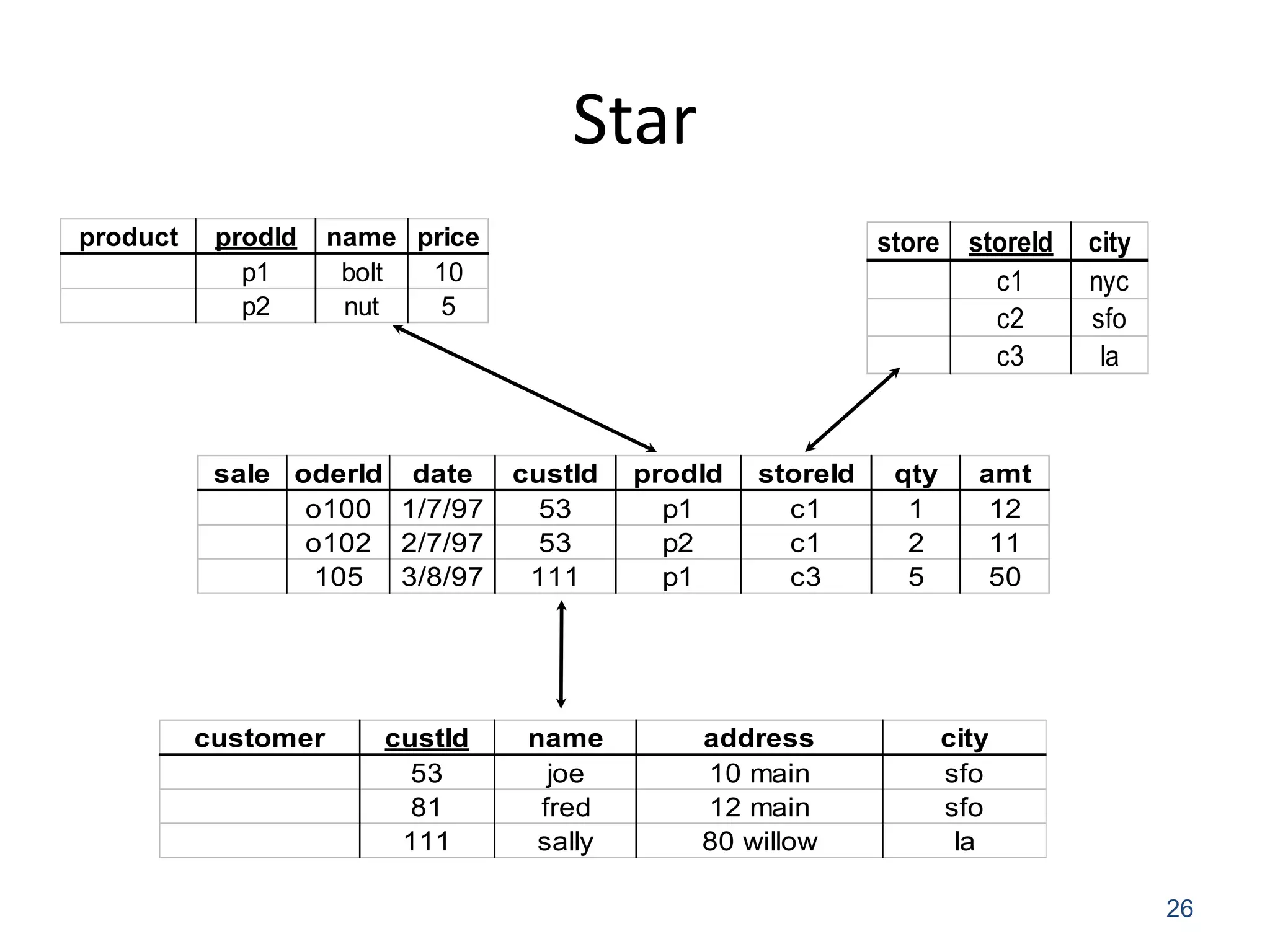
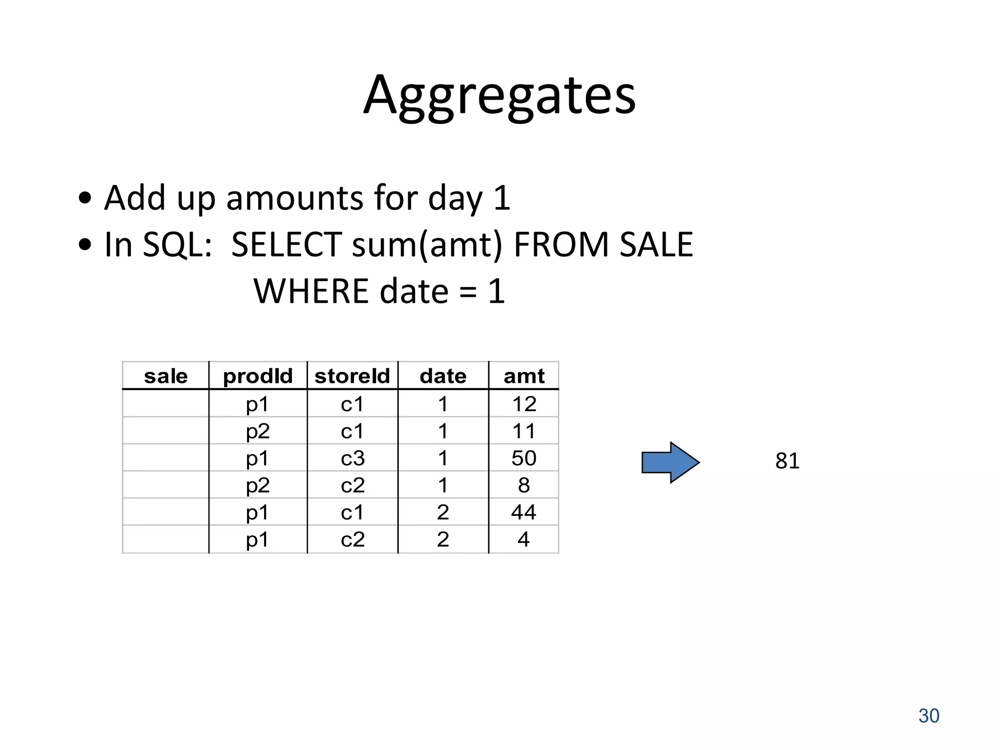
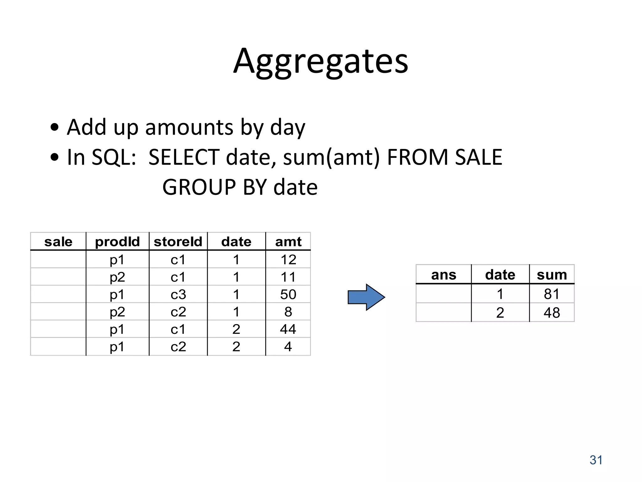
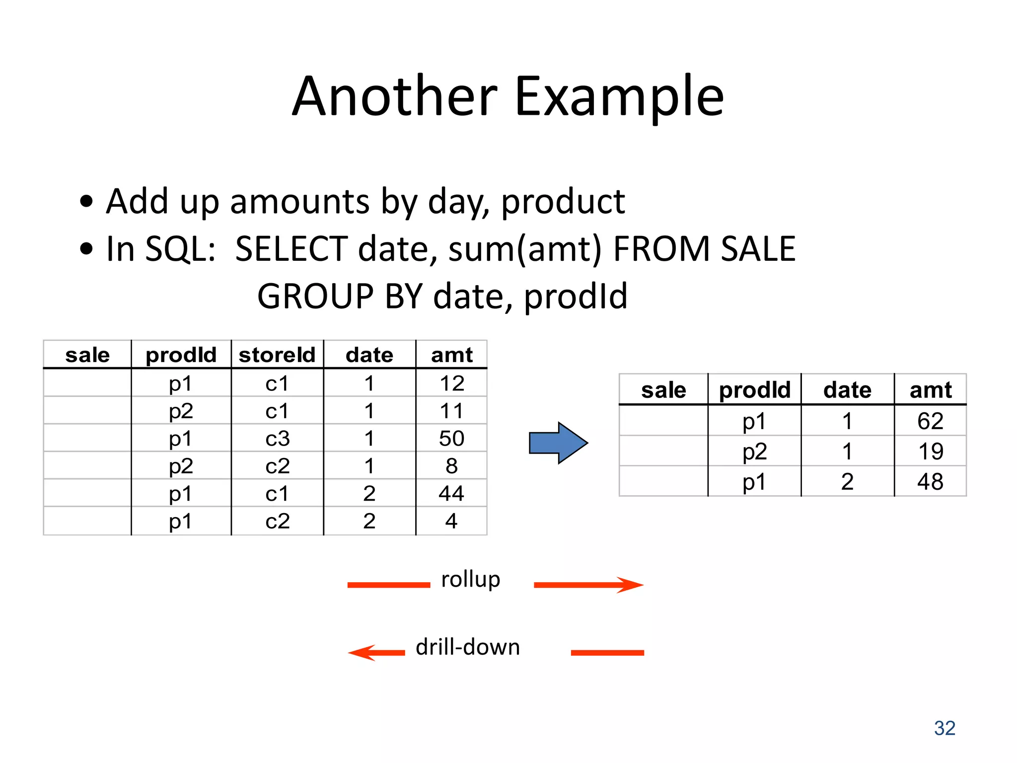
This document provides an introduction to big data and basic data analysis techniques. It discusses the large amounts of data being generated daily from sources like the web, social networks, and scientific projects. It also covers common data types, challenges in working with big data, and some basic statistical and data mining techniques for analyzing large datasets including classification, clustering, and association rule mining.


![[Redis Released]- FalkorDB - Redis + Graph Agentic Memory’s Secret Sauce](https://cdn.slidesharecdn.com/ss_thumbnails/redisreleased-falkordbslidedeck-1125-251115194922-e1c0046b-thumbnail.jpg?width=640&height=640&fit=bounds)


