Download to read offline
![ISSN: 2312-7694
Sakshi et al, / International Journal of Computer and Communication System Engineering (IJCCSE), Vol. 2 (5), 2015, 659-664
659 | P a g e
© IJCCSE All Rights Reserved Vol. 02 No.05 Oct 2015 www.ijccse.com
An Approach of Improvisation in Efficiency of
Apriori Algorithm
Sakshi Aggarwal
SGT Institute of Engineering & Technology
Gurgaon, Haryana
sakshii.26@gmail.com
Dr. Ritu Sindhu
SGT Institute of Engineering & Technology
Gurgaon, Haryana
ritu.sindhu2628@gmail.com
Abstract— Association rule mining is used to find frequent
itemsets in data mining. Classical apriori algorithm is inefficient
due to large scans of the transaction database to find frequent
item sets. In this paper, we are proposing a method to improve
Apriori algorithm efficiency by reducing the database size as well
as reducing the time wasted on scanning the transactions.
Index Terms— Apriori algorithm, Support, Frequent Itemset,
Association rules, Candidate Item
I. INTRODUCTION
Extracting relevant information by exploitation of data is
called Data Mining. There is an increasing need to extract valid
and useful information by business people from large datasets
[2]; here data mining achieves its goal. Thus, data mining has
its importance to discover hidden patterns from huge data
stored in databases, OLAP (Online Analytical Process), data
warehouse etc. [5]. This is the only reason why data mining is
also known as KDD (Knowledge Discovery in Databases). [4]
KDD’s techniques are used to extract the interesting patterns.
Steps of KDD process are cleaning of data (data cleaning),
selecting relevant data, transformation of data, data pre-
processing, mining and pattern evaluation.
II. ASSOCIATION RULE MINING
Association rule mining has its importance in fields of
artificial intelligence, information science, database and many
others. Data volumes are dramatically increasing by day-to-day
activities. Therefore, mining the association rules from massive
data is in the interest for many industries as theses rules help in
decision-making processes, market basket analysis and cross
marketing etc.
Association rule problems are in discussion from 1993 and
many researchers have worked on it to optimize the original
algorithm such as doing random sampling, declining rules,
changing storing framework etc. [1]. We find association rules
from a huge amount of data to identify the relationships in
items which tells about human behavior of buying set of items.
There is always a particular pattern followed by humans during
buying the set of items.
In data mining, unknown dependency in data is found in
association rule mining and then rules between the items are
found [3]. Association rule mining problem is defined as
follows.
DBT = {T1, T2,...,TN } is a database of N T transactions.
Each transaction consists of I, where I= {i1, i2, i3….iN} is a
set of all items. An association rule is of the form A⇒B, where
A and B are item sets, A⊆I, B⊆I, A∩B=∅. The whole point of
an algorithm is to extract the useful information from these
transactions.
For example: Consider below table containing some
transactions:
TABLE I. EXAMPLE OF TRANSACTIONS IN A DATABASE
TID Items
1 CPU, Monitor
2 CPU, Keyboard, Mouse, UPS
3 Monitor, Keyboard, Mouse, Motherboard
4
CPU, Monitor, Keyboard, Mouse
5 CPU, Monitor, Keyboard, Motherboard
Example of Association Rules:
{Keyboard} {Mouse},
{CPU, Monitor} {UPS, Motherboard},
{CPU, Mouse} {Monitor},
A B is an association rule (A and B are itemsets).
Example: {Monitor, Keyboard} {Mouse}
Rule Evaluation:
Support: It is defined as rate of occurrence of an itemset in
a transaction database.
Support (Keyboard Mouse) =
No. Of transactions containing both Keyboard and Mouse
No. Of total transactions
Confidence: For all transactions, it defines the ratio of data
items which contains Y in the items that contains X.](https://image.slidesharecdn.com/rp10155923-160107193637/75/An-Approach-of-Improvisation-in-Efficiency-of-Apriori-Algorithm-1-2048.jpg)
![ISSN: 2312-7694
Sakshi et al, / International Journal of Computer and Communication System Engineering (IJCCSE), Vol. 2 (5), 2015, 659-664
660 | P a g e
© IJCCSE All Rights Reserved Vol. 02 No.05 Oct 2015 www.ijccse.com
Confidence (Keyboard Mouse) =
No. Of transactions containing Keyboard and Mouse
No. Of transactions (containing Keyboard)
Itemset: One or more items collectively are called an
itemset.
Example {Monitor, Keyboard, Mouse}. K-itemset
contains k-items.
Frequent Itemset: For a frequent item set:
SI >= min_sup
Where I is an itemset, min_sup is minimum support
threshold and S represent the support for an itemset.
III. CLASSICAL APRIORI ALGORITHM
Using an iterative approach, in each iteration Apriori
algorithm generates candidate item-sets by using large itemsets
of a previous iteration. [2]. Basic concept of this iterative
approach is as follows:
Algorithm Apriori_algo(Lk)
1. L1= {frequent-1 item-sets};
2. for (k=2; Lk-1≠Φ; k++) {
3. Ck= generate_Apriori(Lk-1); //New candidates
4. forall transactions t ϵ D do begin
5. Ct=subset(Ck,t); //Candidates contained in t
6. forall candidates c ϵ Ct do
7. c.count++;
8. }
9. Lk={c ϵ Ck | c.count≥minsup}
10. end for
11. Answer=UkLk
Algorithm 1: Apriori Algorithm [6]
Above algorithm is the apriori algorithm. In above,
database is scanned to find frequent 1-itemsets along with the
count of each item. Frequent itemset L1 is created from
candidate item set where each item satisfies minimum support.
In next each iteration, set of item sets is used as a seed which
is used to generate next set of large itemsets i.e candidate item
sets (candidate generation) using apriori_gen function.
Lk-1 is input to generate_Apriori function and returns Ck.
Join step joins Lk-1 with another Lk-1 and in prune step, item
sets
c ϵ Ck are deleted such that (k-1) is the subset of “c” but not
in Lk-1 of Ck-1.
Algorithm generate_Apriori (Lk)
1. insert into Ck
2. p=Lk-1 ,q= Lk-1
3. select p.I1,p.I2,.....p.Ik-1,q.Ik-1 from p,q
where p.I1=q.I1.....p.Ik-2= q.Ik-2,p.Ik-1<q.Ik-1;
4. forall itemsets c ϵ Ck do
5. forall { s ⊃ (k-1) of c) do
6. if(s ∉ Lk-1) then
7. from Ck , delete c
Algorithm 2: Apriori-Gen Function[6]
Fig 1: Apriori Algoithm Steps
A. Limitations of Apriori Algorithm
Large number of candidate and frequent item sets are
to be handled and results in increased cost and waste of
time.
Example: if number of frequent (k-1) items is 104
then
almost 107
Ck need to be generated and tested [2]. So
scanning of a database is done many times to find Ck.
Apriori is inefficient in terms of memory requirement
when large numbers of transactions are in
consideration.](https://image.slidesharecdn.com/rp10155923-160107193637/75/An-Approach-of-Improvisation-in-Efficiency-of-Apriori-Algorithm-2-2048.jpg)
![ISSN: 2312-7694
Sakshi et al, / International Journal of Computer and Communication System Engineering (IJCCSE), Vol. 2 (5), 2015, 659-664
664 | P a g e
© IJCCSE All Rights Reserved Vol. 02 No.05 Oct 2015 www.ijccse.com
Fig 13: Comparative Analysis
VII. CONCLUSION
We have proposed an idea to improve the efficiency of
apriori algorithm by reducing the time taken to scan database
transactions. We find that with increase in value of k, number
of transactions scanned decreases and thus, time consumed
also decreases in comparison to classical apriori algorithm.
Because of this, time taken to generate candidate item sets
in our idea also decreases in comparison to classical apriori.
REFERENCES
[1] J. Han and M. Kamber, Conception and Technology of Data
Mining, Beijing: China Machine Press, 2007.
[2] U. Fayyad, G. Piatetsky-Shapiro, and P. Smyth, “From data
mining to knowledge discovery in databases,” vol. 17, no. 3, AI
magazine, 1996, pp. 37.
[3] S. Rao, R. Gupta, “Implementing Improved Algorithm over
APRIORI Data Mining Association Rule Algorithm”,
International Journal of Computer Science And Technology, pp.
489-493, Mar. 2012
[4] H. H. O. Nasereddin, “Stream data mining,” International
Journal of Web Applications, vol. 1, no. 4,pp. 183–190, 2009.
[5] M. Halkidi, “Quality assessment and uncertainty handling in
data mining process,” in Proc, EDBT Conference, Konstanz,
Germany, 2000.
[6] Rakesh Agarwal, Ramakrishna Srikant, “Fast Algorithm for
mining association rules” VLDB Conference Santiago, Chile,
1994, pp 487-499.](https://image.slidesharecdn.com/rp10155923-160107193637/75/An-Approach-of-Improvisation-in-Efficiency-of-Apriori-Algorithm-6-2048.jpg)
![ISSN: 2312-7694
Sakshi et al, / International Journal of Computer and Communication System Engineering (IJCCSE), Vol. 2 (5), 2015, 659-664
659 | P a g e
© IJCCSE All Rights Reserved Vol. 02 No.05 Oct 2015 www.ijccse.com
An Approach of Improvisation in Efficiency of
Apriori Algorithm
Sakshi Aggarwal
SGT Institute of Engineering & Technology
Gurgaon, Haryana
sakshii.26@gmail.com
Dr. Ritu Sindhu
SGT Institute of Engineering & Technology
Gurgaon, Haryana
ritu.sindhu2628@gmail.com
Abstract— Association rule mining is used to find frequent
itemsets in data mining. Classical apriori algorithm is inefficient
due to large scans of the transaction database to find frequent
item sets. In this paper, we are proposing a method to improve
Apriori algorithm efficiency by reducing the database size as well
as reducing the time wasted on scanning the transactions.
Index Terms— Apriori algorithm, Support, Frequent Itemset,
Association rules, Candidate Item
I. INTRODUCTION
Extracting relevant information by exploitation of data is
called Data Mining. There is an increasing need to extract valid
and useful information by business people from large datasets
[2]; here data mining achieves its goal. Thus, data mining has
its importance to discover hidden patterns from huge data
stored in databases, OLAP (Online Analytical Process), data
warehouse etc. [5]. This is the only reason why data mining is
also known as KDD (Knowledge Discovery in Databases). [4]
KDD’s techniques are used to extract the interesting patterns.
Steps of KDD process are cleaning of data (data cleaning),
selecting relevant data, transformation of data, data pre-
processing, mining and pattern evaluation.
II. ASSOCIATION RULE MINING
Association rule mining has its importance in fields of
artificial intelligence, information science, database and many
others. Data volumes are dramatically increasing by day-to-day
activities. Therefore, mining the association rules from massive
data is in the interest for many industries as theses rules help in
decision-making processes, market basket analysis and cross
marketing etc.
Association rule problems are in discussion from 1993 and
many researchers have worked on it to optimize the original
algorithm such as doing random sampling, declining rules,
changing storing framework etc. [1]. We find association rules
from a huge amount of data to identify the relationships in
items which tells about human behavior of buying set of items.
There is always a particular pattern followed by humans during
buying the set of items.
In data mining, unknown dependency in data is found in
association rule mining and then rules between the items are
found [3]. Association rule mining problem is defined as
follows.
DBT = {T1, T2,...,TN } is a database of N T transactions.
Each transaction consists of I, where I= {i1, i2, i3….iN} is a
set of all items. An association rule is of the form A⇒B, where
A and B are item sets, A⊆I, B⊆I, A∩B=∅. The whole point of
an algorithm is to extract the useful information from these
transactions.
For example: Consider below table containing some
transactions:
TABLE I. EXAMPLE OF TRANSACTIONS IN A DATABASE
TID Items
1 CPU, Monitor
2 CPU, Keyboard, Mouse, UPS
3 Monitor, Keyboard, Mouse, Motherboard
4
CPU, Monitor, Keyboard, Mouse
5 CPU, Monitor, Keyboard, Motherboard
Example of Association Rules:
{Keyboard} {Mouse},
{CPU, Monitor} {UPS, Motherboard},
{CPU, Mouse} {Monitor},
A B is an association rule (A and B are itemsets).
Example: {Monitor, Keyboard} {Mouse}
Rule Evaluation:
Support: It is defined as rate of occurrence of an itemset in
a transaction database.
Support (Keyboard Mouse) =
No. Of transactions containing both Keyboard and Mouse
No. Of total transactions
Confidence: For all transactions, it defines the ratio of data
items which contains Y in the items that contains X.](https://crownmelresort.com/image.slidesharecdn.com/rp10155923-160107193637/75/An-Approach-of-Improvisation-in-Efficiency-of-Apriori-Algorithm-1-2048.jpg)
![ISSN: 2312-7694
Sakshi et al, / International Journal of Computer and Communication System Engineering (IJCCSE), Vol. 2 (5), 2015, 659-664
660 | P a g e
© IJCCSE All Rights Reserved Vol. 02 No.05 Oct 2015 www.ijccse.com
Confidence (Keyboard Mouse) =
No. Of transactions containing Keyboard and Mouse
No. Of transactions (containing Keyboard)
Itemset: One or more items collectively are called an
itemset.
Example {Monitor, Keyboard, Mouse}. K-itemset
contains k-items.
Frequent Itemset: For a frequent item set:
SI >= min_sup
Where I is an itemset, min_sup is minimum support
threshold and S represent the support for an itemset.
III. CLASSICAL APRIORI ALGORITHM
Using an iterative approach, in each iteration Apriori
algorithm generates candidate item-sets by using large itemsets
of a previous iteration. [2]. Basic concept of this iterative
approach is as follows:
Algorithm Apriori_algo(Lk)
1. L1= {frequent-1 item-sets};
2. for (k=2; Lk-1≠Φ; k++) {
3. Ck= generate_Apriori(Lk-1); //New candidates
4. forall transactions t ϵ D do begin
5. Ct=subset(Ck,t); //Candidates contained in t
6. forall candidates c ϵ Ct do
7. c.count++;
8. }
9. Lk={c ϵ Ck | c.count≥minsup}
10. end for
11. Answer=UkLk
Algorithm 1: Apriori Algorithm [6]
Above algorithm is the apriori algorithm. In above,
database is scanned to find frequent 1-itemsets along with the
count of each item. Frequent itemset L1 is created from
candidate item set where each item satisfies minimum support.
In next each iteration, set of item sets is used as a seed which
is used to generate next set of large itemsets i.e candidate item
sets (candidate generation) using apriori_gen function.
Lk-1 is input to generate_Apriori function and returns Ck.
Join step joins Lk-1 with another Lk-1 and in prune step, item
sets
c ϵ Ck are deleted such that (k-1) is the subset of “c” but not
in Lk-1 of Ck-1.
Algorithm generate_Apriori (Lk)
1. insert into Ck
2. p=Lk-1 ,q= Lk-1
3. select p.I1,p.I2,.....p.Ik-1,q.Ik-1 from p,q
where p.I1=q.I1.....p.Ik-2= q.Ik-2,p.Ik-1<q.Ik-1;
4. forall itemsets c ϵ Ck do
5. forall { s ⊃ (k-1) of c) do
6. if(s ∉ Lk-1) then
7. from Ck , delete c
Algorithm 2: Apriori-Gen Function[6]
Fig 1: Apriori Algoithm Steps
A. Limitations of Apriori Algorithm
Large number of candidate and frequent item sets are
to be handled and results in increased cost and waste of
time.
Example: if number of frequent (k-1) items is 104
then
almost 107
Ck need to be generated and tested [2]. So
scanning of a database is done many times to find Ck.
Apriori is inefficient in terms of memory requirement
when large numbers of transactions are in
consideration.](https://crownmelresort.com/image.slidesharecdn.com/rp10155923-160107193637/75/An-Approach-of-Improvisation-in-Efficiency-of-Apriori-Algorithm-2-2048.jpg)


![ISSN: 2312-7694
Sakshi et al, / International Journal of Computer and Communication System Engineering (IJCCSE), Vol. 2 (5), 2015, 659-664
664 | P a g e
© IJCCSE All Rights Reserved Vol. 02 No.05 Oct 2015 www.ijccse.com
Fig 13: Comparative Analysis
VII. CONCLUSION
We have proposed an idea to improve the efficiency of
apriori algorithm by reducing the time taken to scan database
transactions. We find that with increase in value of k, number
of transactions scanned decreases and thus, time consumed
also decreases in comparison to classical apriori algorithm.
Because of this, time taken to generate candidate item sets
in our idea also decreases in comparison to classical apriori.
REFERENCES
[1] J. Han and M. Kamber, Conception and Technology of Data
Mining, Beijing: China Machine Press, 2007.
[2] U. Fayyad, G. Piatetsky-Shapiro, and P. Smyth, “From data
mining to knowledge discovery in databases,” vol. 17, no. 3, AI
magazine, 1996, pp. 37.
[3] S. Rao, R. Gupta, “Implementing Improved Algorithm over
APRIORI Data Mining Association Rule Algorithm”,
International Journal of Computer Science And Technology, pp.
489-493, Mar. 2012
[4] H. H. O. Nasereddin, “Stream data mining,” International
Journal of Web Applications, vol. 1, no. 4,pp. 183–190, 2009.
[5] M. Halkidi, “Quality assessment and uncertainty handling in
data mining process,” in Proc, EDBT Conference, Konstanz,
Germany, 2000.
[6] Rakesh Agarwal, Ramakrishna Srikant, “Fast Algorithm for
mining association rules” VLDB Conference Santiago, Chile,
1994, pp 487-499.](https://crownmelresort.com/image.slidesharecdn.com/rp10155923-160107193637/75/An-Approach-of-Improvisation-in-Efficiency-of-Apriori-Algorithm-6-2048.jpg)
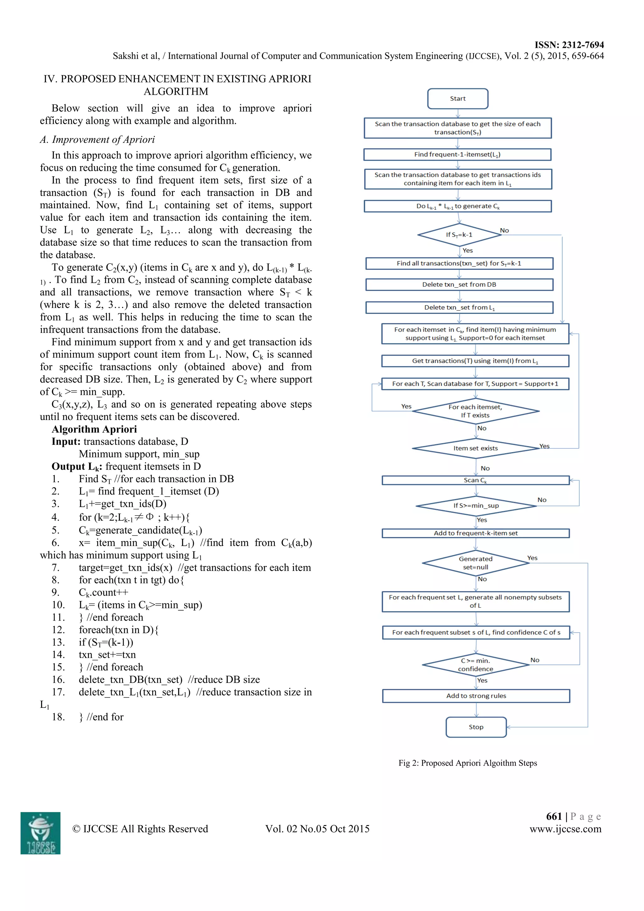
This document proposes an approach to improve the efficiency of the Apriori algorithm for association rule mining. The Apriori algorithm is inefficient because it requires multiple scans of the transaction database to find frequent itemsets. The proposed approach aims to reduce this inefficiency in two ways: 1) It reduces the size of the transaction database by removing transactions where the transaction size is less than the candidate itemset size. 2) It scans only the relevant transactions for candidate itemset counting rather than the full database, by using transaction IDs of minimum support items from the first pass of the algorithm. An example is provided to demonstrate how the approach reduces the database and number of transactions scanned to generate frequent itemsets more efficiently than the standard Apriori