Download as PDF, PPTX

![7
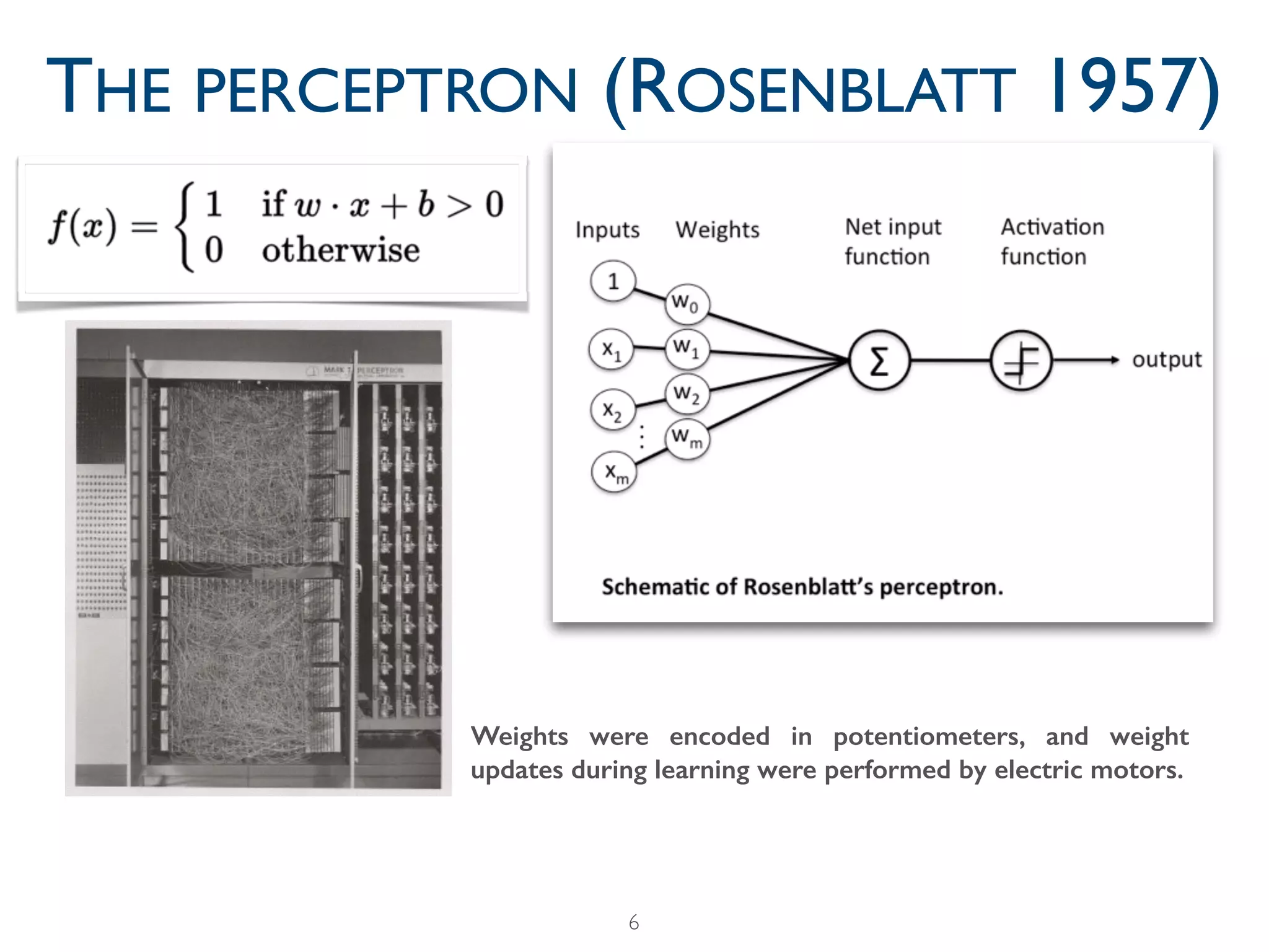
THE PERCEPTRON (ROSENBLATT 1957)
Based on Rosenblatt's
statements, The New York
Times reported the perceptron
to be "the embryo of an
electronic computer that [the
Navy] expects will be able to
walk, talk, see, write, reproduce
itself and be conscious of its
existence."](https://image.slidesharecdn.com/slidesdeeplearningintro-170917112542/75/A-historical-introduction-to-deep-learning-hardware-data-and-tricks-7-2048.jpg)


![7
THE PERCEPTRON (ROSENBLATT 1957)
Based on Rosenblatt's
statements, The New York
Times reported the perceptron
to be "the embryo of an
electronic computer that [the
Navy] expects will be able to
walk, talk, see, write, reproduce
itself and be conscious of its
existence."](https://crownmelresort.com/image.slidesharecdn.com/slidesdeeplearningintro-170917112542/75/A-historical-introduction-to-deep-learning-hardware-data-and-tricks-7-2048.jpg)


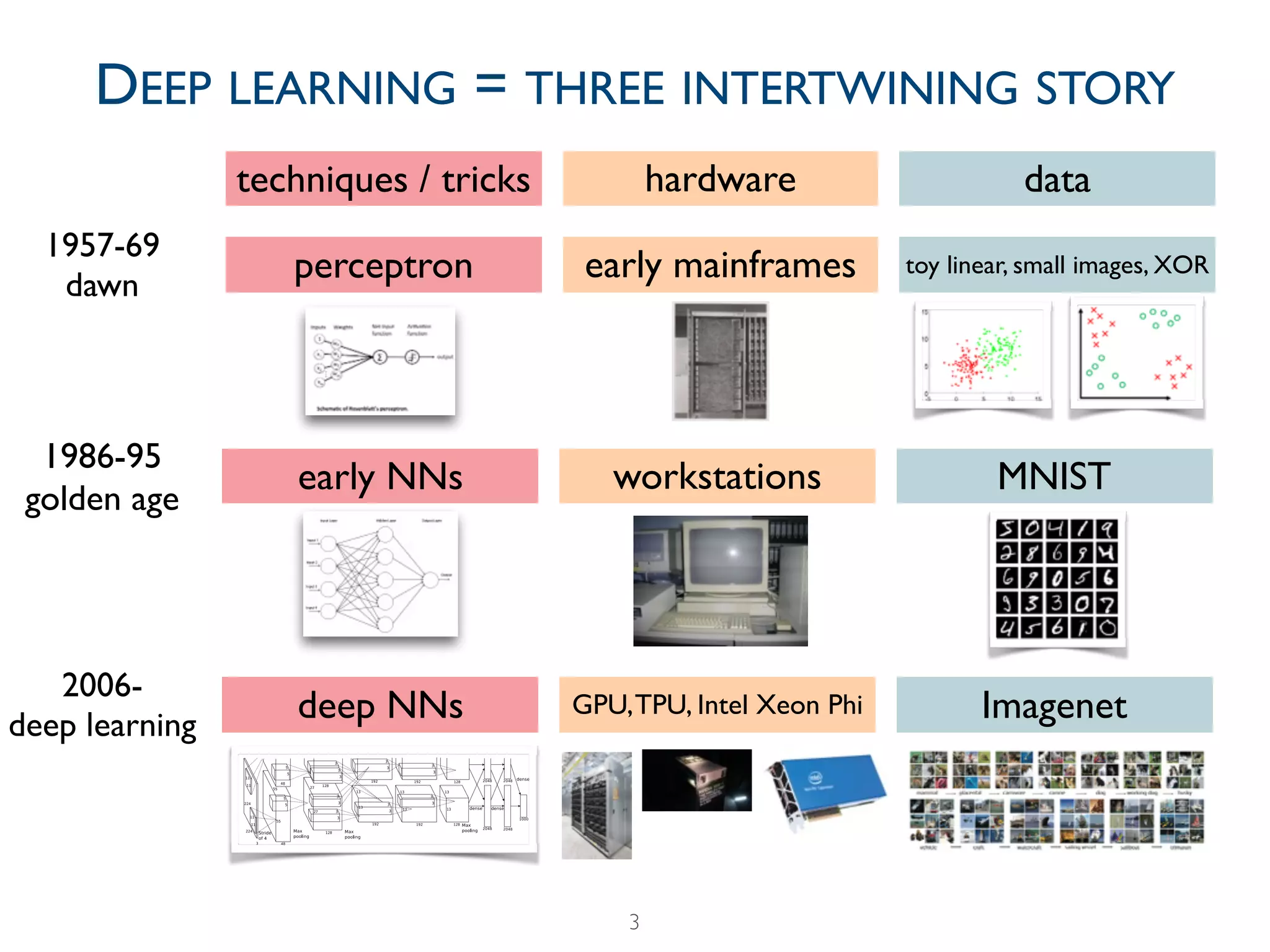
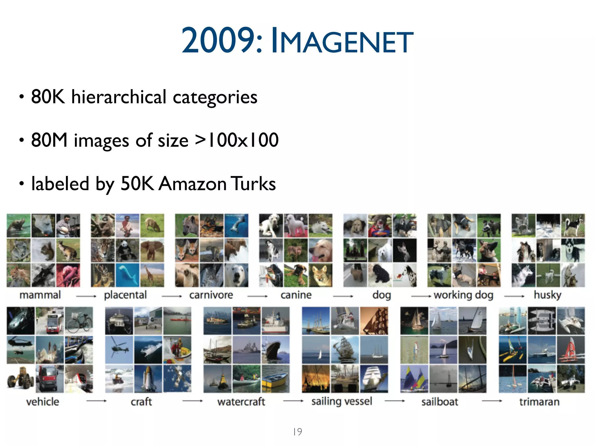
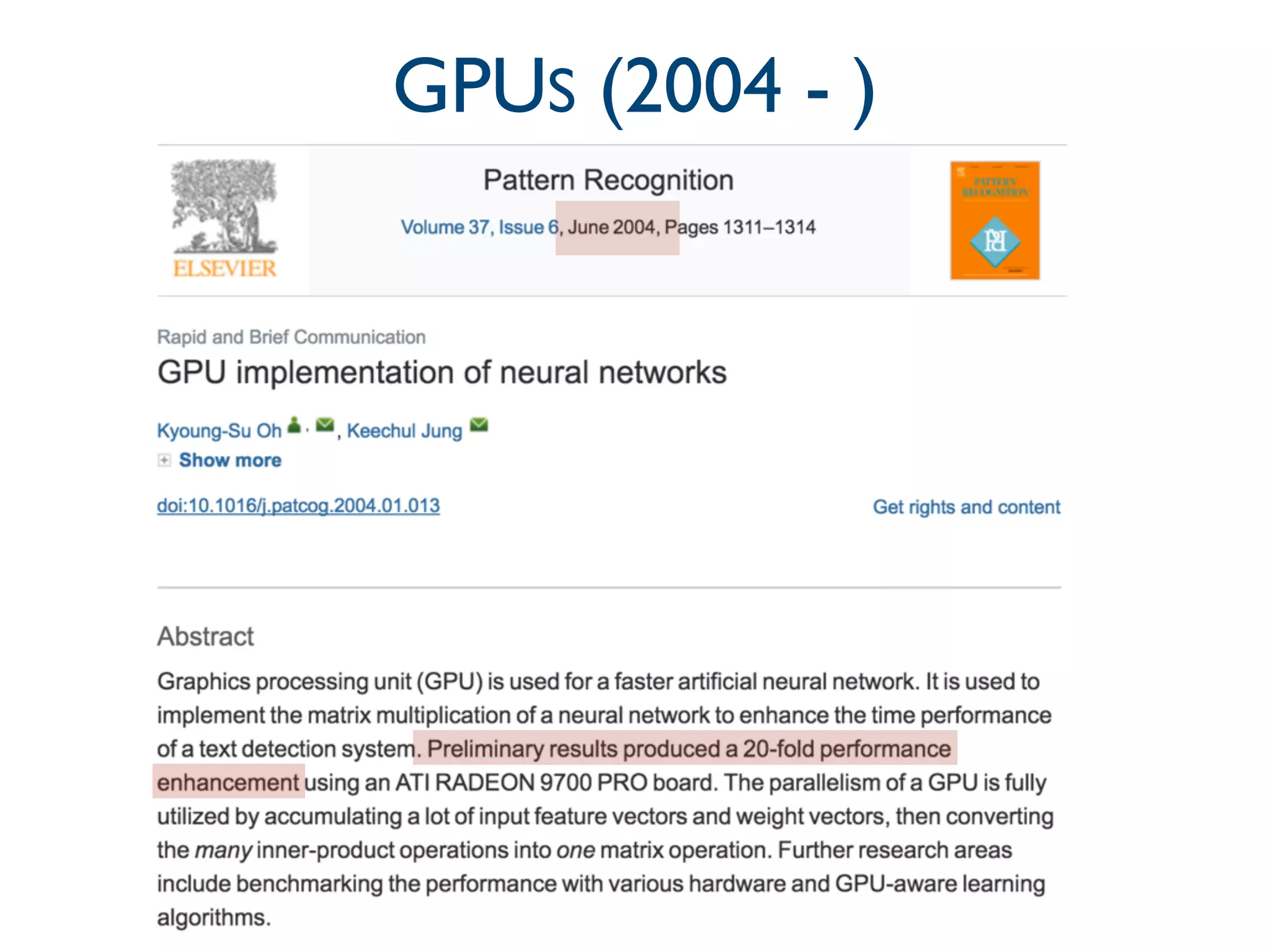
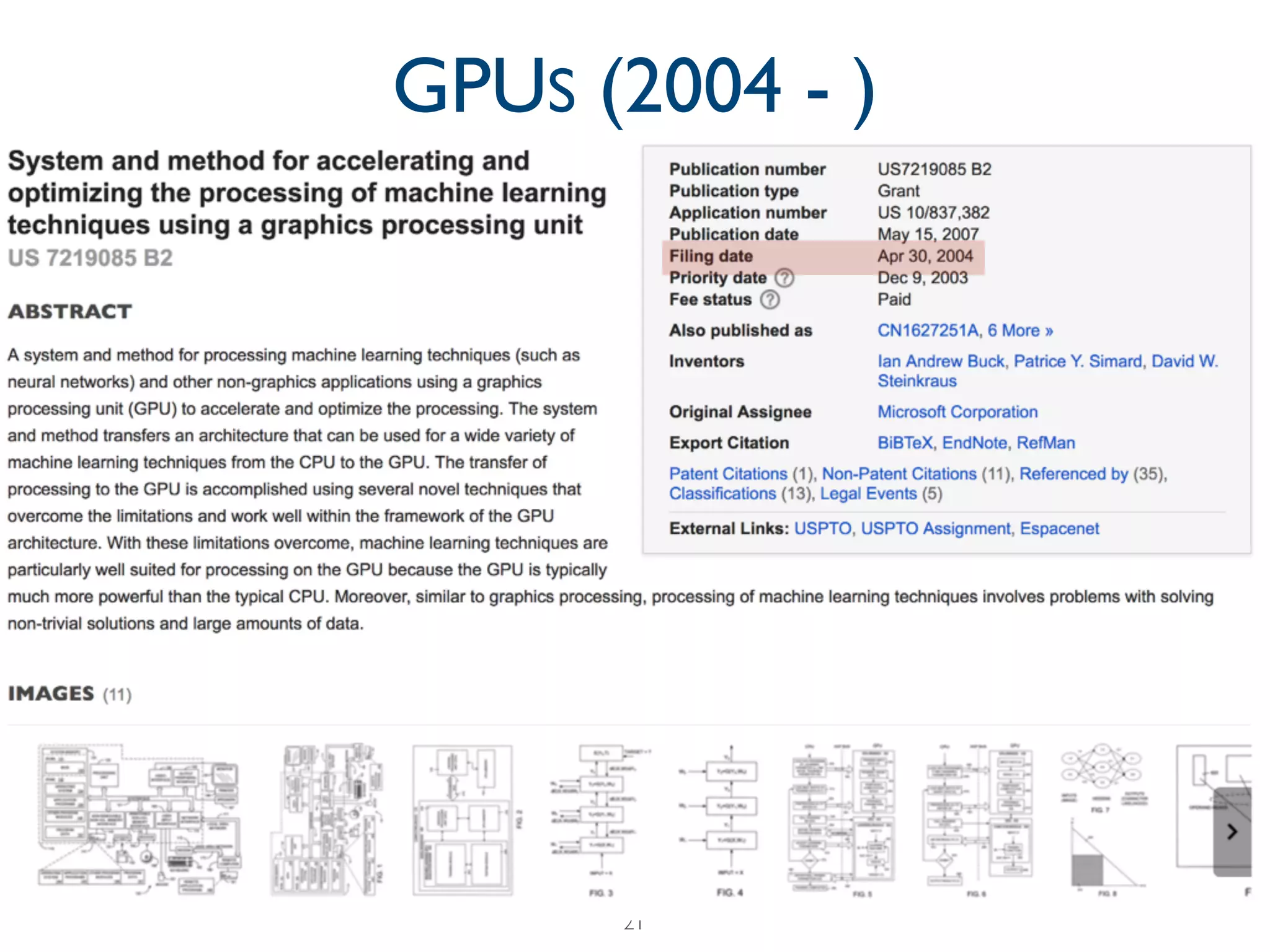
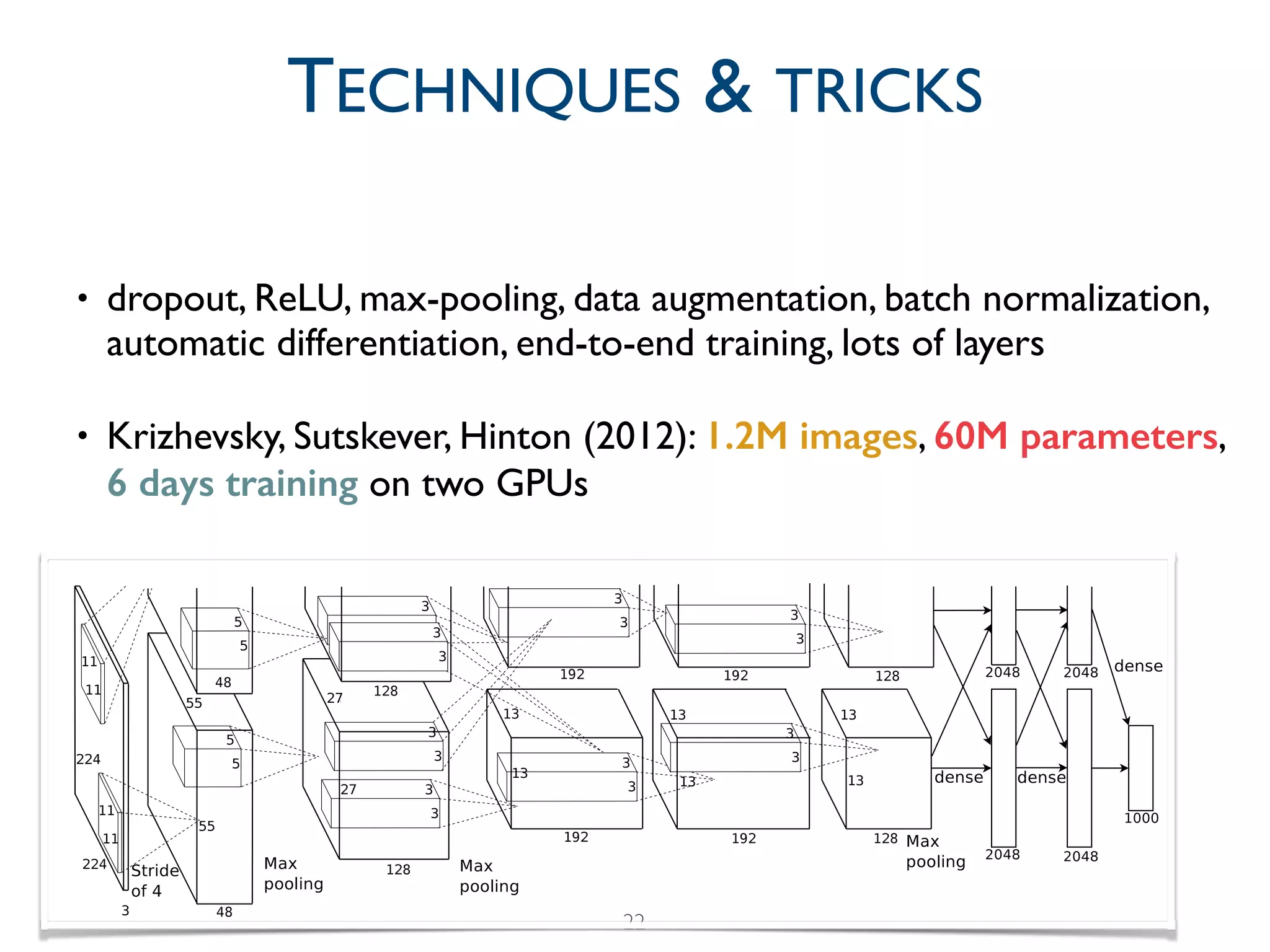
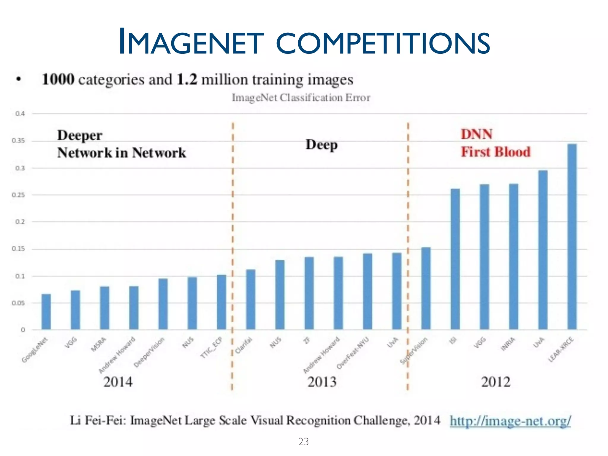
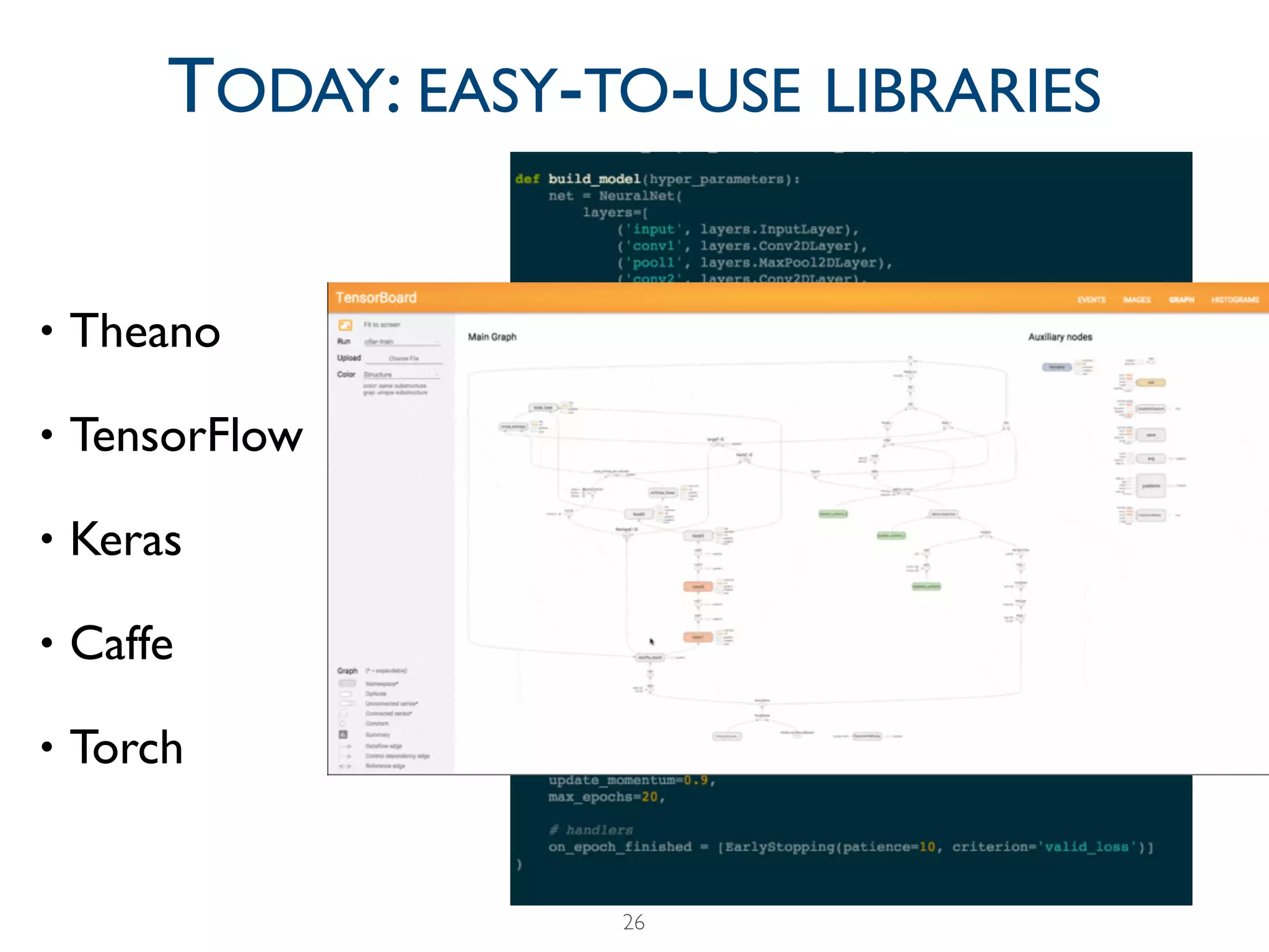
The document provides a comprehensive overview of the evolution of deep learning, detailing its historical development from early perceptrons to modern architectures utilizing GPUs and large datasets. It highlights key milestones, including the challenges faced during the 'AI winters' and the resurgence of neural networks from 2006 onwards, notably with the introduction of ImageNet. Additionally, it emphasizes the importance of data and computational power in training deep learning models, alongside contemporary tools used in the field.