Downloaded 163 times


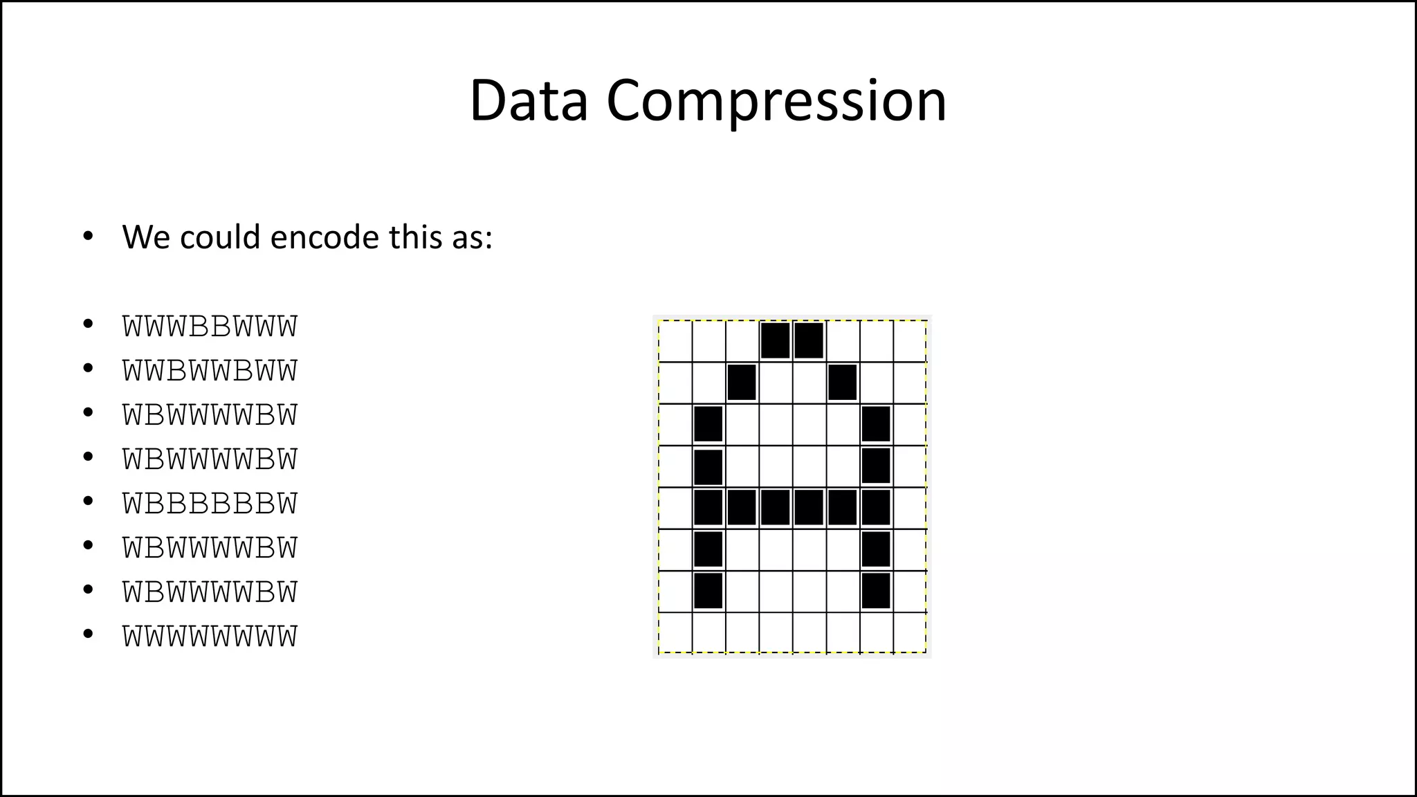
![Boolean Logic
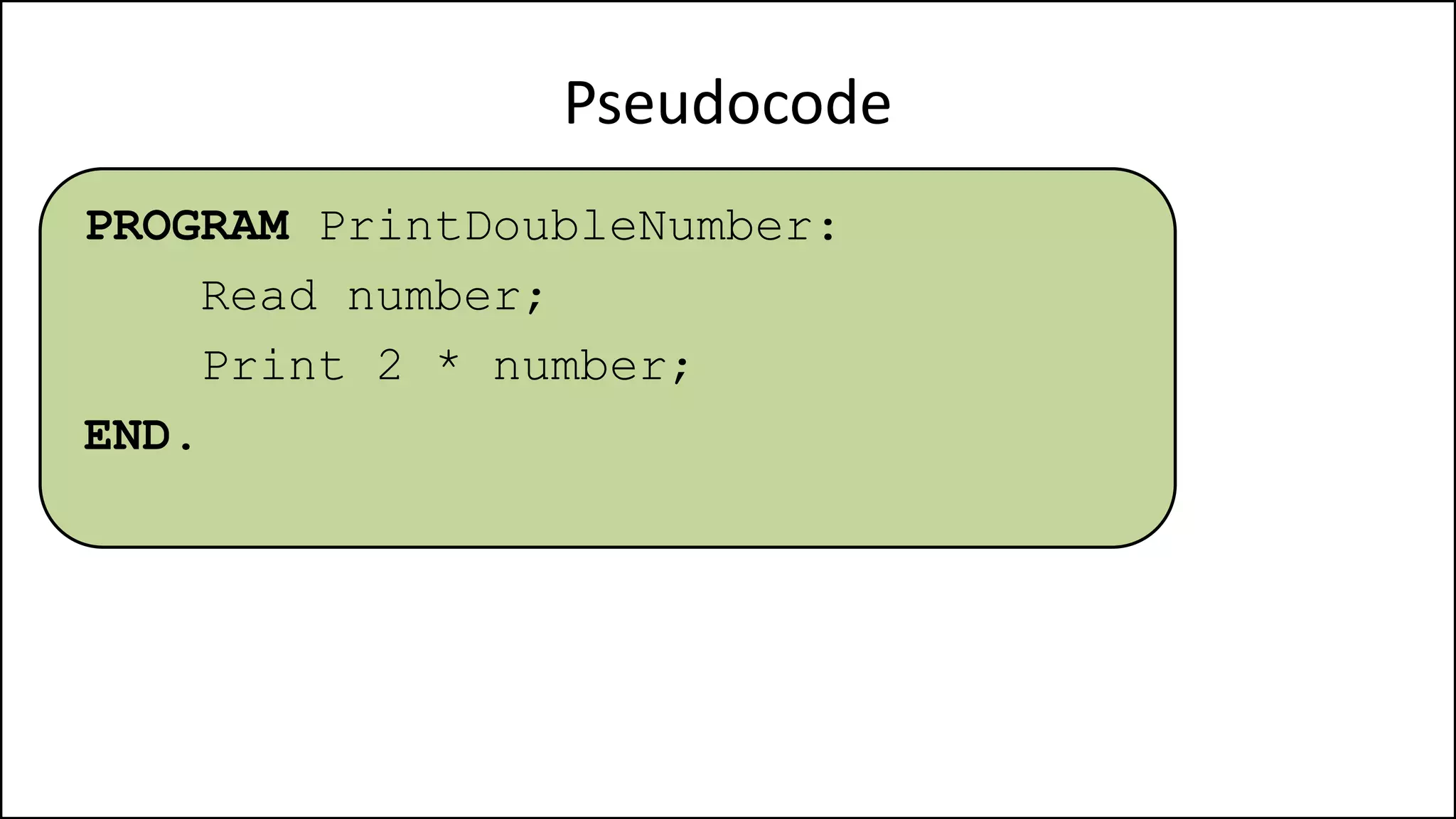
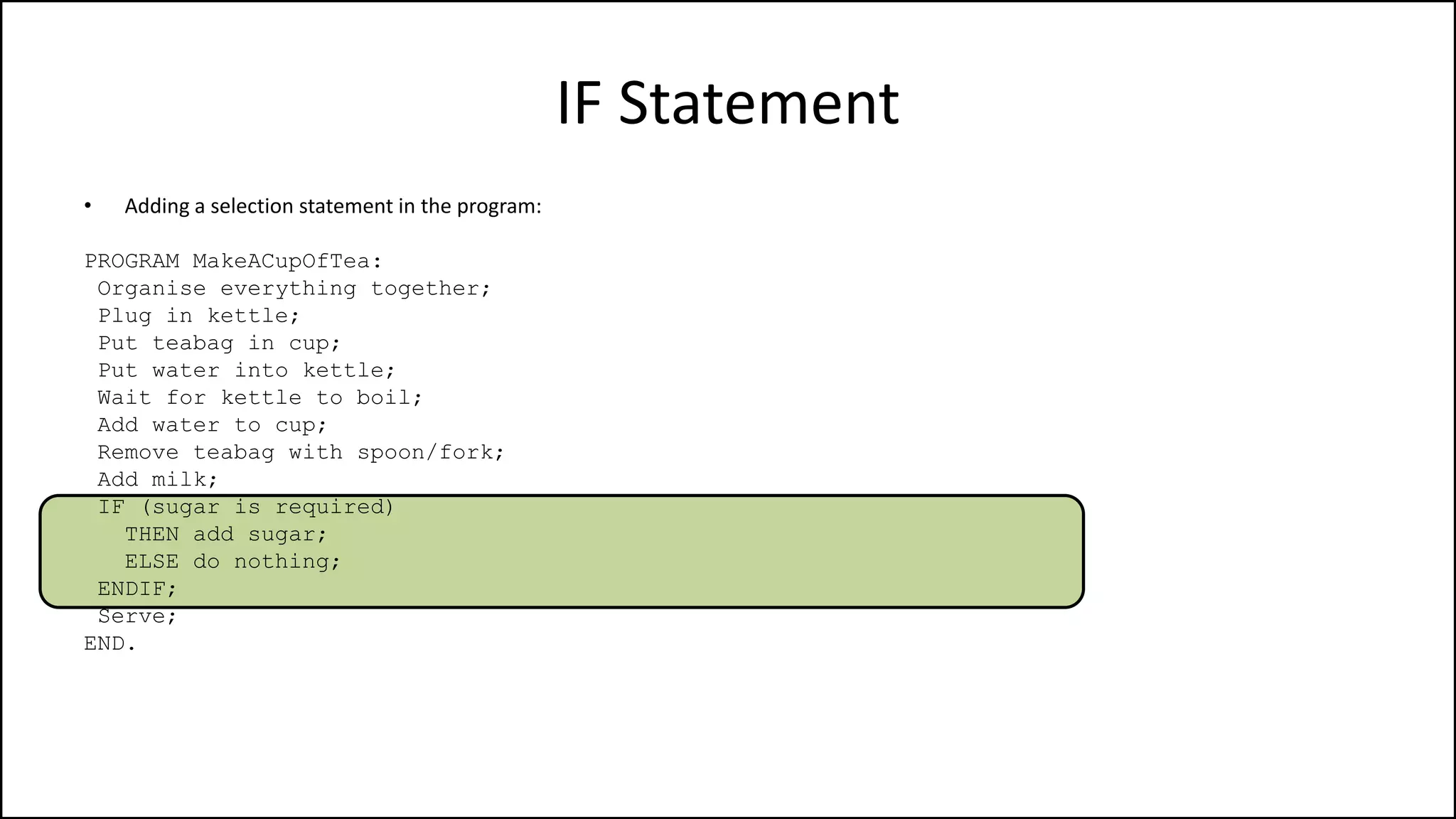
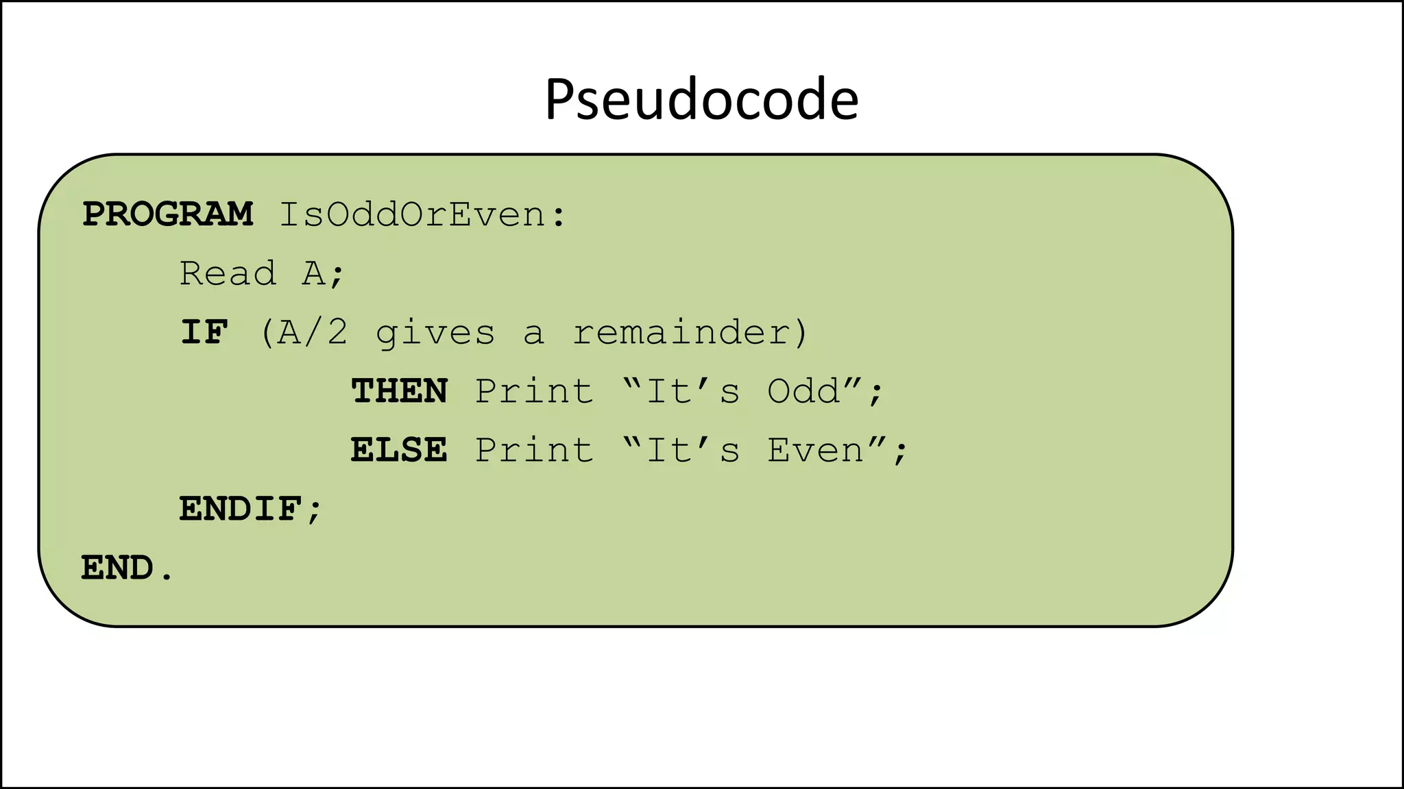
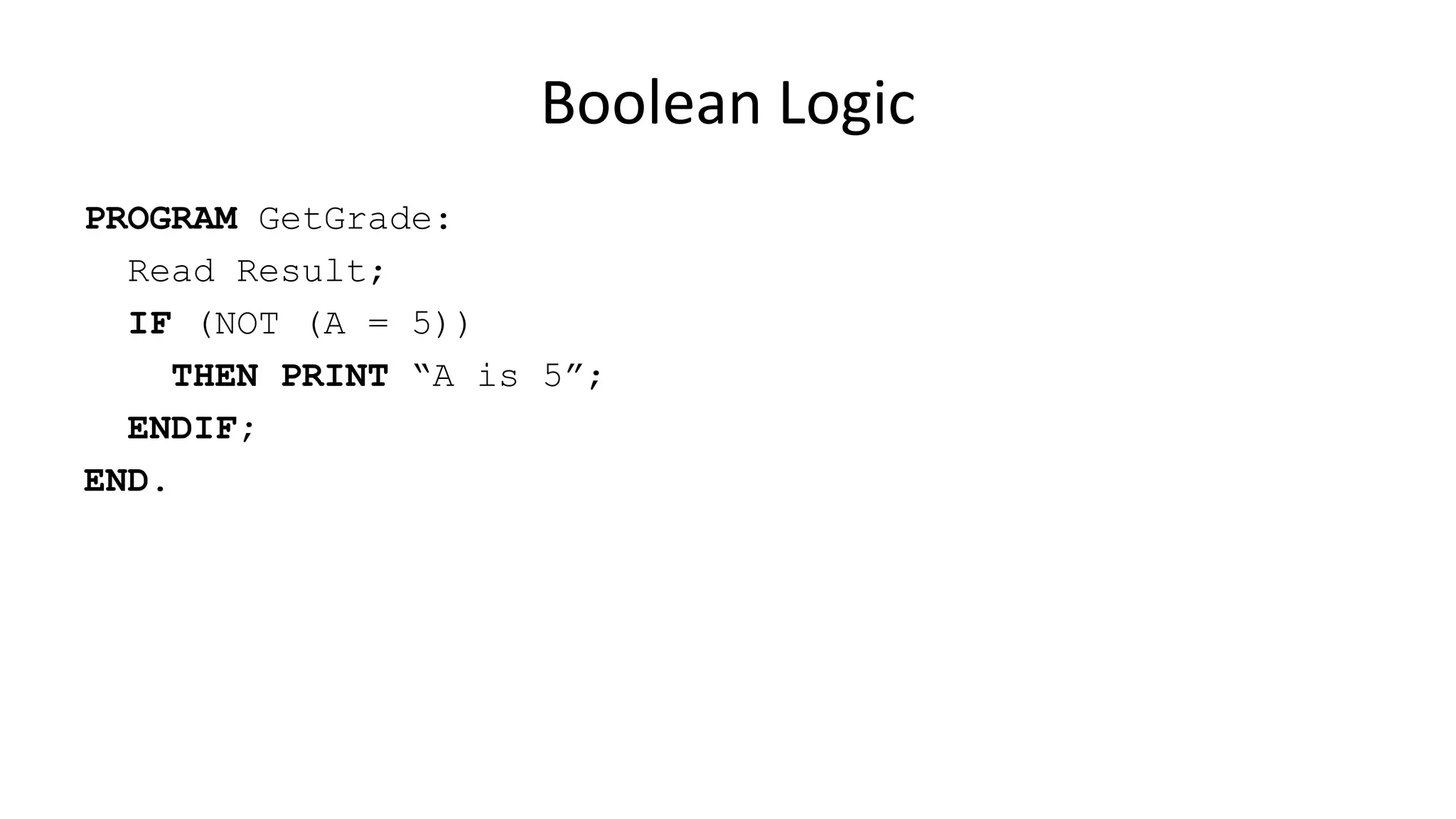
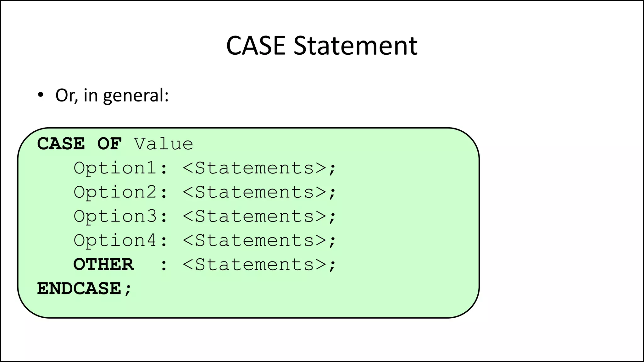
PROGRAM GetGrade:
Read Result;
IF (A = 5 AND Age[Index] < Age[Index+1])
THEN PRINT “A is 5”;
ENDIF;
END.](https://image.slidesharecdn.com/completecourse-150726101701-lva1-app6892/75/A-complete-course-in-Program-Design-using-Pseudocode-154-2048.jpg)
![Boolean Logic
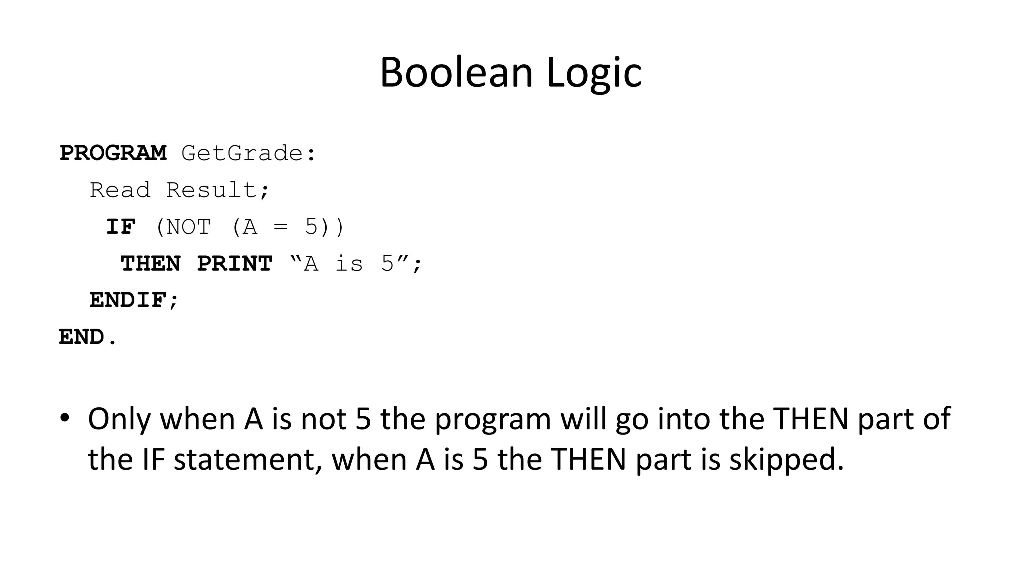
PROGRAM GetGrade:
Read Result;
IF (A = 5 AND Age[Index] < Age[Index+1])
THEN PRINT “A is 5”;
ENDIF;
END.
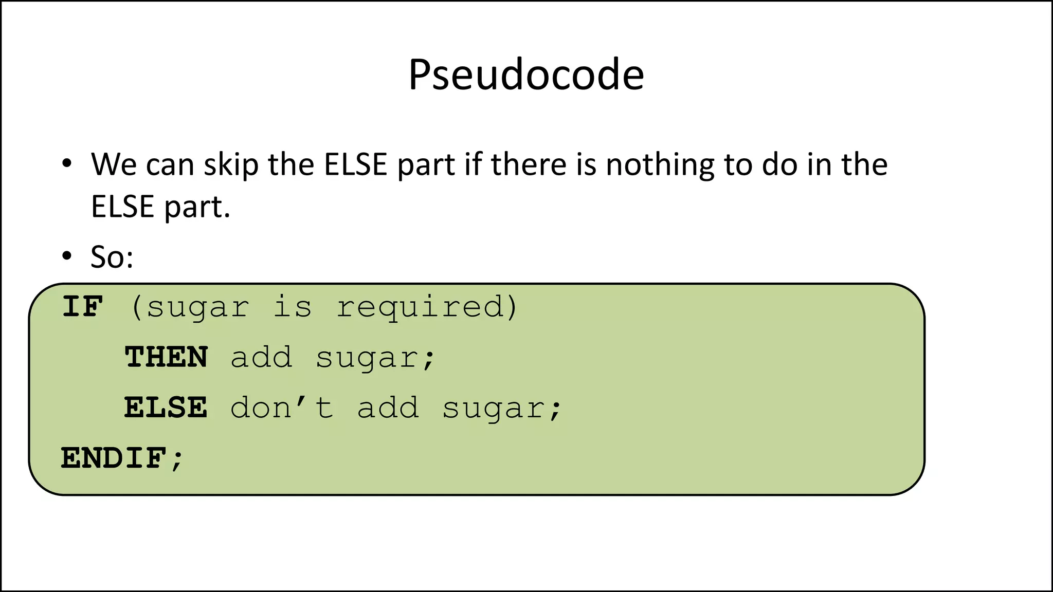
• Both A=5 and Age[Index] < Age[Index+1] must be
TRUE to do the THEN part of the statement.](https://image.slidesharecdn.com/completecourse-150726101701-lva1-app6892/75/A-complete-course-in-Program-Design-using-Pseudocode-155-2048.jpg)
![Boolean Logic
PROGRAM GetGrade:
Read Result;
IF (A = 5 OR Age[Index] < Age[Index+1])
THEN PRINT “A is 5”;
ENDIF;
END.](https://image.slidesharecdn.com/completecourse-150726101701-lva1-app6892/75/A-complete-course-in-Program-Design-using-Pseudocode-157-2048.jpg)
![Boolean Logic
PROGRAM GetGrade:
Read Result;
IF (A = 5 OR Age[Index] < Age[Index+1])
THEN PRINT “A is 5”;
ENDIF;
END.
• Either or both of A=5 and Age[Index] <
Age[Index+1] must be TRUE to do the THEN part of the
statement.](https://image.slidesharecdn.com/completecourse-150726101701-lva1-app6892/75/A-complete-course-in-Program-Design-using-Pseudocode-158-2048.jpg)


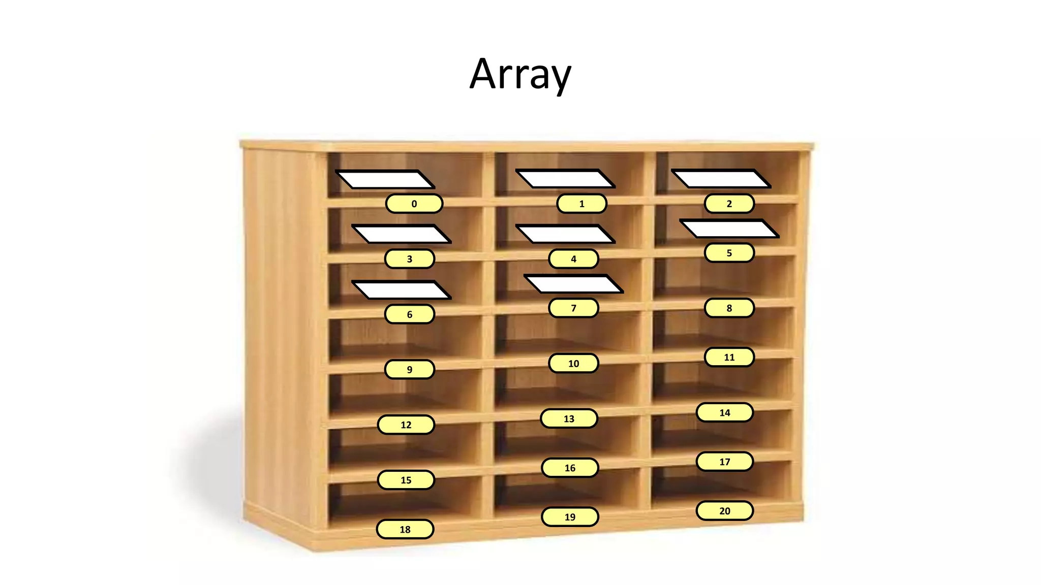
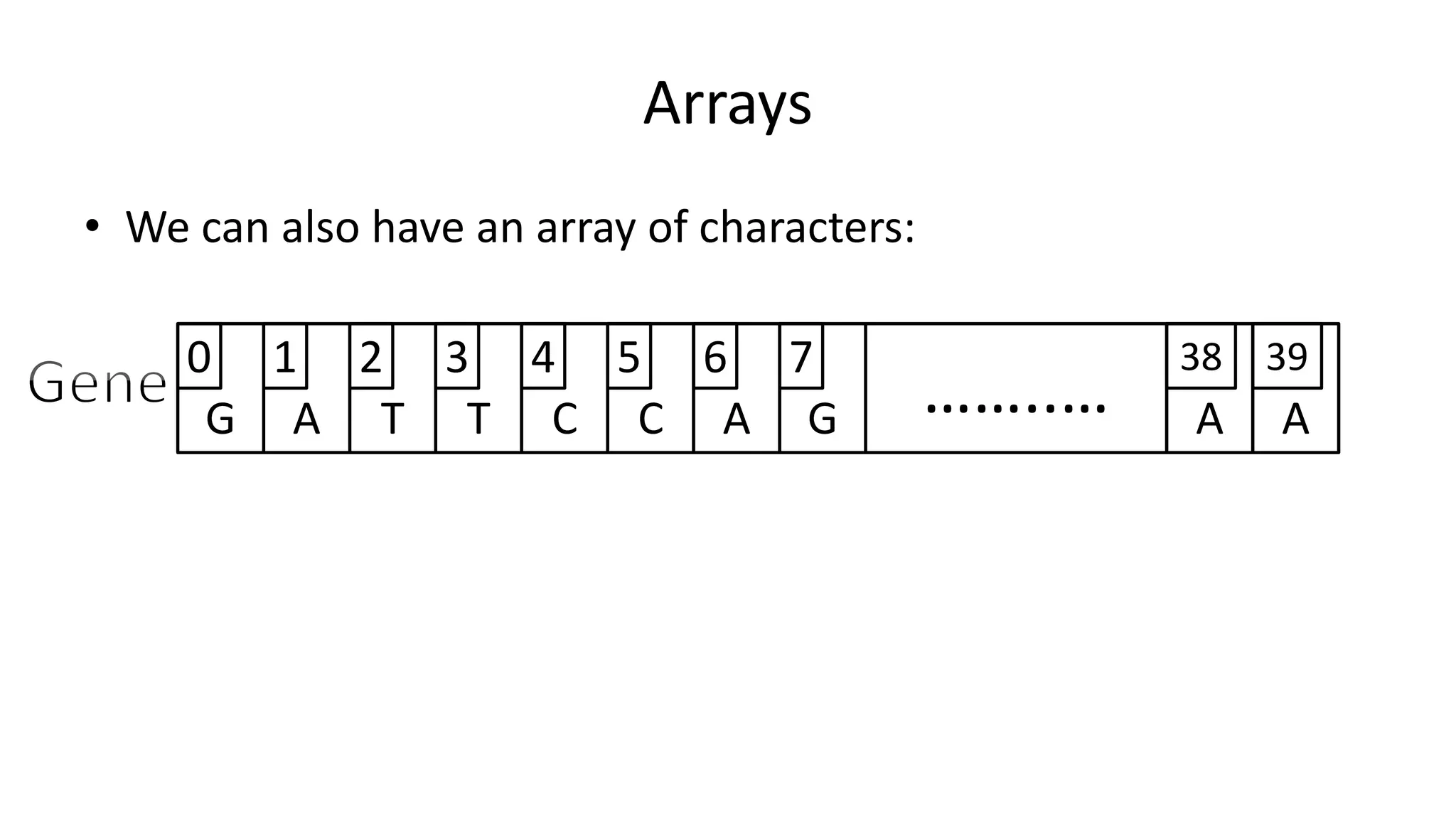
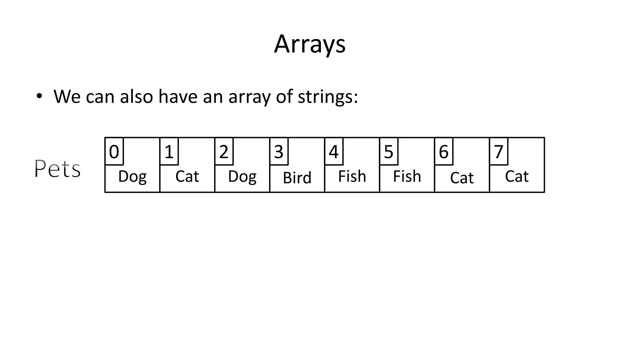
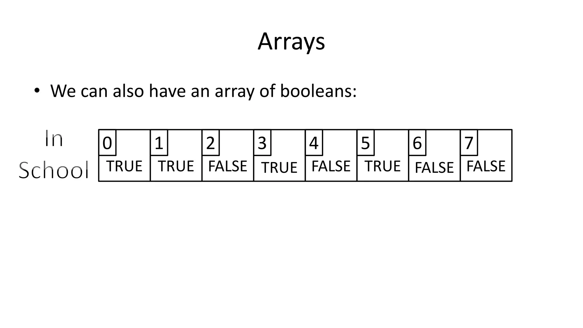
![Arrays
• We declare an array as follows:
• Integer Age[40];](https://image.slidesharecdn.com/completecourse-150726101701-lva1-app6892/75/A-complete-course-in-Program-Design-using-Pseudocode-325-2048.jpg)
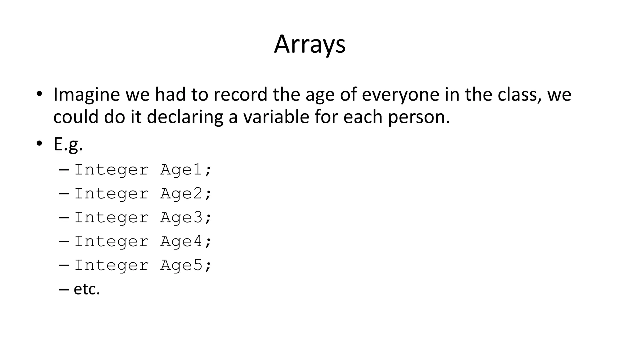
![Arrays
• We declare an array as follows:
• Integer Age[40];
• Which means we declare 40 integer variables, all can be
accessed using the Age name.
……..…](https://image.slidesharecdn.com/completecourse-150726101701-lva1-app6892/75/A-complete-course-in-Program-Design-using-Pseudocode-326-2048.jpg)
![Arrays
• We declare an array as follows:
• Integer Age[40];
• Which means we declare 40 integer variables, all can be
accessed using the Age name.
0 1 2 3 4 5 6 397 ……..… 38](https://image.slidesharecdn.com/completecourse-150726101701-lva1-app6892/75/A-complete-course-in-Program-Design-using-Pseudocode-327-2048.jpg)
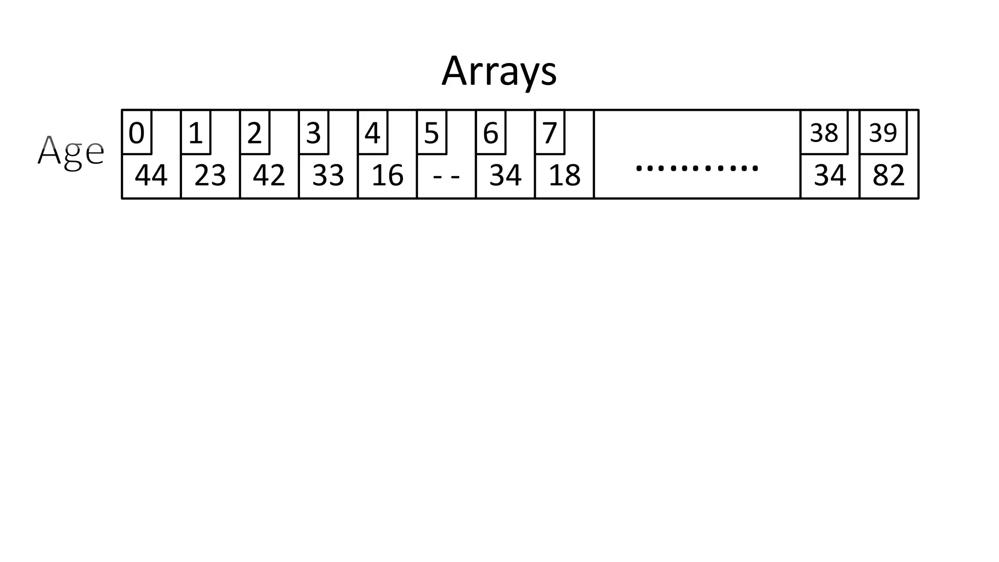
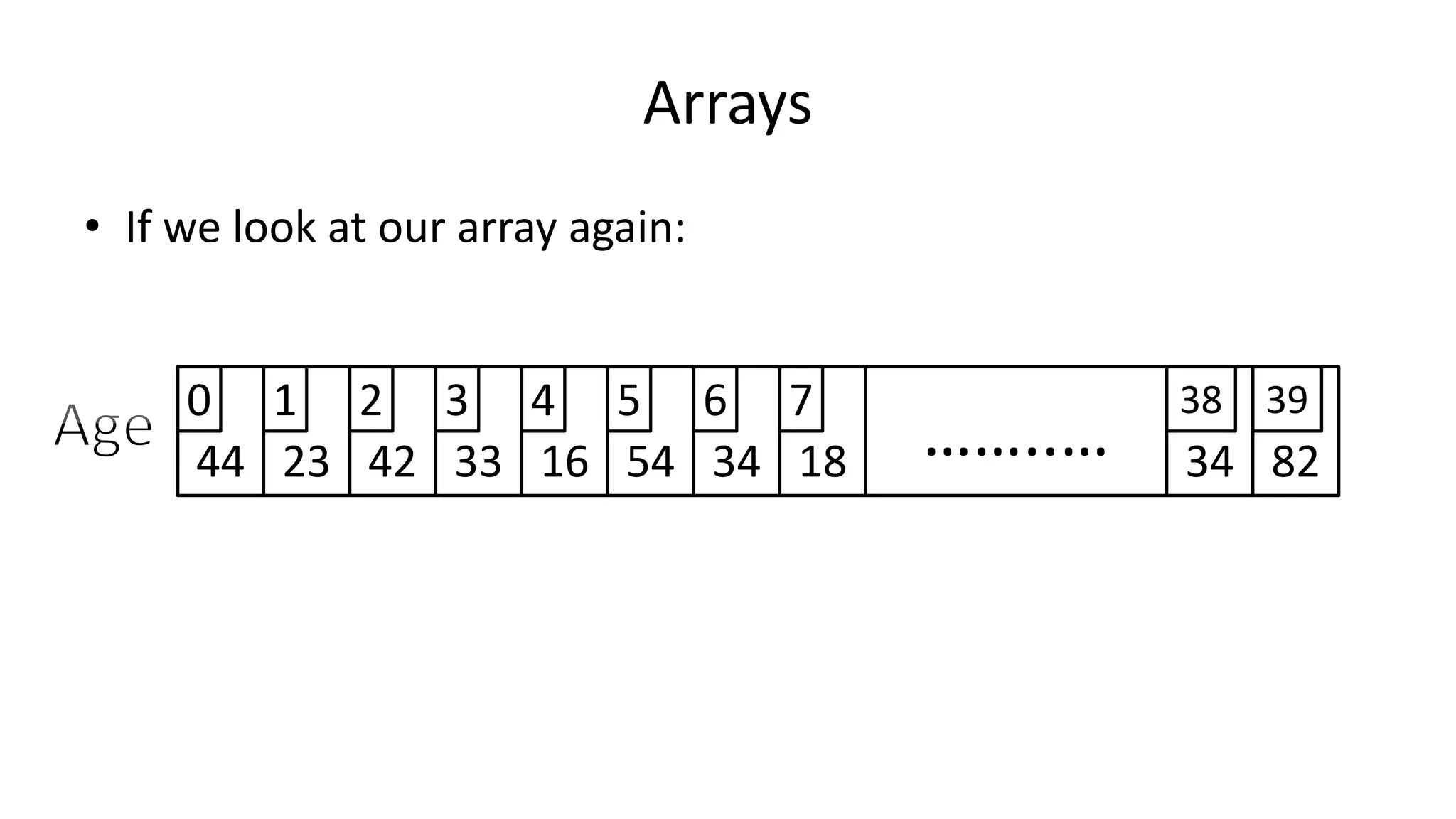
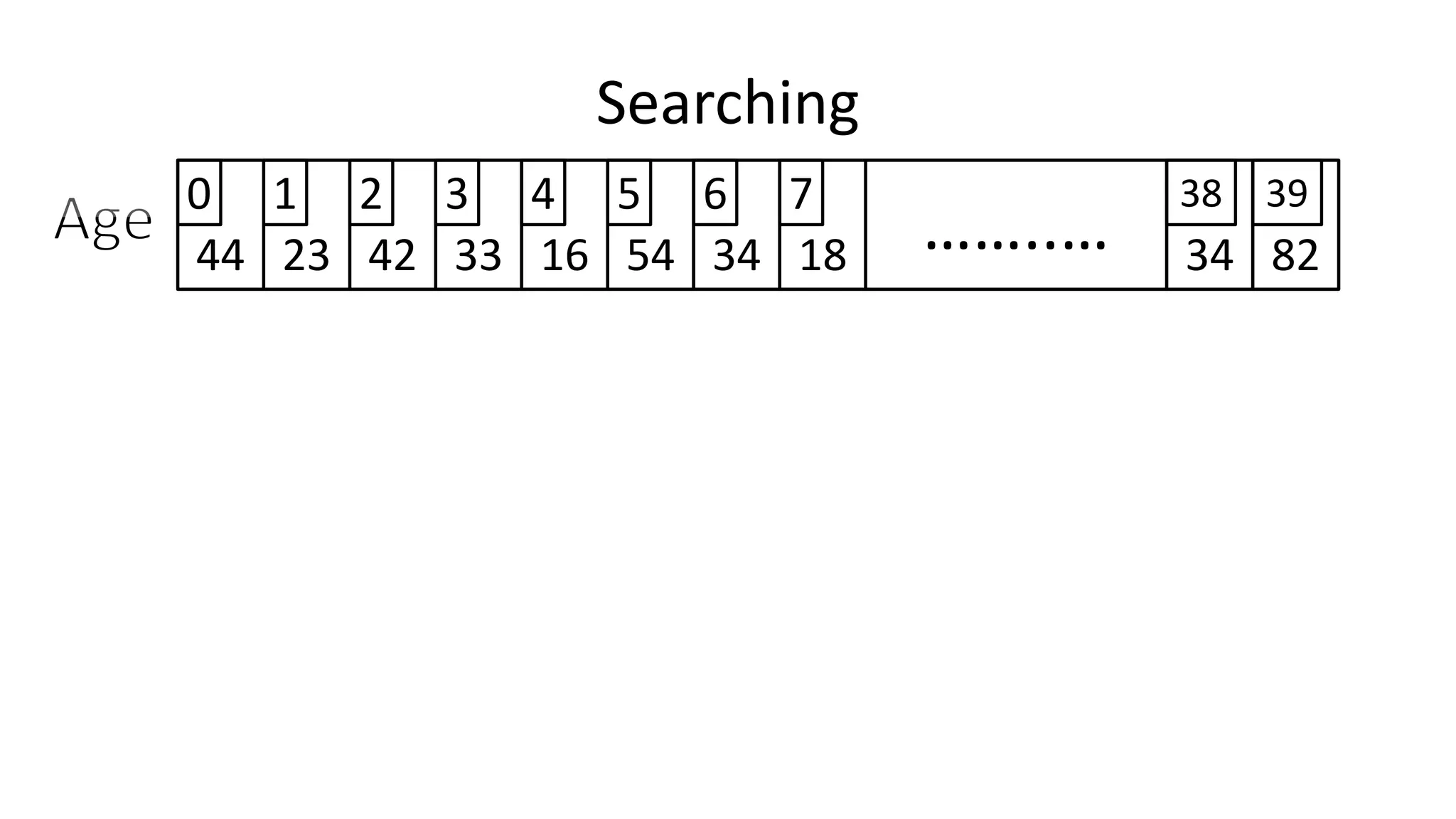
![Arrays
44 23 42 33 16 - - 34 8218 ……..… 34
0 1 2 3 4 5 6 7 38 39
• So if I do:
• PRINT Age[0];
• We will get:
• 44](https://image.slidesharecdn.com/completecourse-150726101701-lva1-app6892/75/A-complete-course-in-Program-Design-using-Pseudocode-329-2048.jpg)
![Arrays
44 23 42 33 16 - - 34 8218 ……..… 34
0 1 2 3 4 5 6 7 38 39
• So if I do:
• PRINT Age[2];
• We will get:
• 42](https://image.slidesharecdn.com/completecourse-150726101701-lva1-app6892/75/A-complete-course-in-Program-Design-using-Pseudocode-330-2048.jpg)
![Arrays
44 23 42 33 16 - - 34 8218 ……..… 34
0 1 2 3 4 5 6 7 38 39
• So if I do:
• PRINT Age[39];
• We will get:
• 82](https://image.slidesharecdn.com/completecourse-150726101701-lva1-app6892/75/A-complete-course-in-Program-Design-using-Pseudocode-331-2048.jpg)
![Arrays
44 23 42 33 16 - - 34 8218 ……..… 34
0 1 2 3 4 5 6 7 38 39
• So if I do:
• PRINT Age[40];
• We will get:
• Array Out of Bounds Exception](https://image.slidesharecdn.com/completecourse-150726101701-lva1-app6892/75/A-complete-course-in-Program-Design-using-Pseudocode-332-2048.jpg)
![Arrays
44 23 42 33 16 - - 34 8218 ……..… 34
0 1 2 3 4 5 6 7 38 39
• We notice that Age[5] is blank.
• If I want to put a value into it (e.g. 54), I do:
• Age[5] <- 54;](https://image.slidesharecdn.com/completecourse-150726101701-lva1-app6892/75/A-complete-course-in-Program-Design-using-Pseudocode-333-2048.jpg)
![Arrays
44 23 42 33 16 54 34 8218 ……..… 34
0 1 2 3 4 5 6 7 38 39
• We notice that Age[5] is blank.
• If I want to put a value into it (e.g. 54), I do:
• Age[5] <- 54;](https://image.slidesharecdn.com/completecourse-150726101701-lva1-app6892/75/A-complete-course-in-Program-Design-using-Pseudocode-334-2048.jpg)

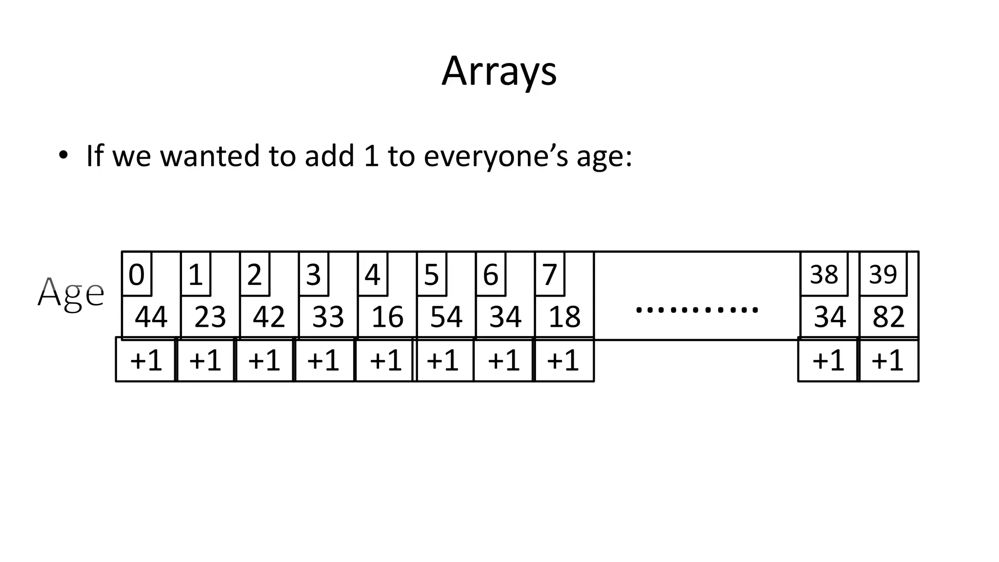
![Arrays
• We could do it like this:
PROGRAM Add1ToAge:
Age[0] <- Age[0] + 1;
Age[1] <- Age[1] + 1;
Age[2] <- Age[2] + 1;
Age[3] <- Age[3] + 1;
Age[4] <- Age[4] + 1;
Age[5] <- Age[5] + 1;
………………………………………………………
Age[38] <- Age[38] + 1;
Age[39] <- Age[39] + 1;
END.](https://image.slidesharecdn.com/completecourse-150726101701-lva1-app6892/75/A-complete-course-in-Program-Design-using-Pseudocode-340-2048.jpg)
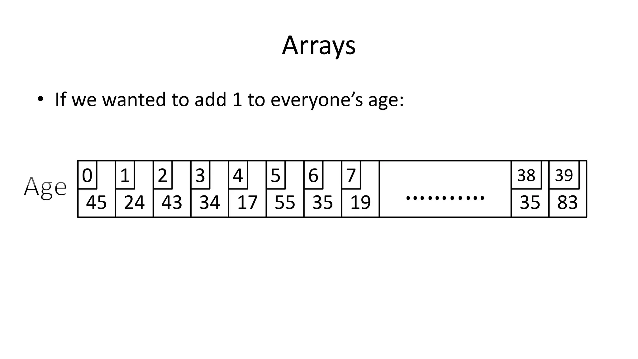
![Arrays
• An easier way of doing it is:
PROGRAM Add1ToAge:
N <- 0;
WHILE (N != 40)
DO Age[N] <- Age[N] + 1;
N <- N + 1;
ENDWHILE;
END.](https://image.slidesharecdn.com/completecourse-150726101701-lva1-app6892/75/A-complete-course-in-Program-Design-using-Pseudocode-341-2048.jpg)
![Arrays
• Or:
PROGRAM Add1ToAge:
FOR N IN 0 TO 39
DO Age[N] <- Age[N] + 1;
ENDFOR;
END.](https://image.slidesharecdn.com/completecourse-150726101701-lva1-app6892/75/A-complete-course-in-Program-Design-using-Pseudocode-342-2048.jpg)
![Arrays
• If we want to add up all the values in the array:
PROGRAM TotalOfArray:
integer Total <- 0;
FOR N IN 0 TO 39
DO Total <- Total + Age[N];
ENDFOR;
END.](https://image.slidesharecdn.com/completecourse-150726101701-lva1-app6892/75/A-complete-course-in-Program-Design-using-Pseudocode-344-2048.jpg)
![Arrays
• So the average age is:
PROGRAM AverageOfArray:
integer Total <- 0;
FOR N IN 0 TO 39
DO Total <- Total + Age[N];
ENDFOR;
PRINT Total/40;
END.](https://image.slidesharecdn.com/completecourse-150726101701-lva1-app6892/75/A-complete-course-in-Program-Design-using-Pseudocode-346-2048.jpg)
![Arrays
• We can add another variable:
PROGRAM AverageOfArray:
integer Total <- 0;
integer ArraySize <- 40;
FOR N IN 0 TO 39
DO Total <- Total + Age[N];
ENDFOR;
PRINT Total/40;
END.](https://image.slidesharecdn.com/completecourse-150726101701-lva1-app6892/75/A-complete-course-in-Program-Design-using-Pseudocode-347-2048.jpg)
![Arrays
• We can add another variable:
PROGRAM AverageOfArray:
integer Total <- 0;
integer ArraySize <- 40;
FOR N IN 0 TO 39
DO Total <- Total + Age[N];
ENDFOR;
PRINT Total/ArraySize;
END.](https://image.slidesharecdn.com/completecourse-150726101701-lva1-app6892/75/A-complete-course-in-Program-Design-using-Pseudocode-348-2048.jpg)
![Arrays
• We can add another variable:
PROGRAM AverageOfArray:
integer Total <- 0;
integer ArraySize <- 40;
FOR N IN 0 TO ArraySize-1
DO Total <- Total + Age[N];
ENDFOR;
PRINT Total/ArraySize;
END.](https://image.slidesharecdn.com/completecourse-150726101701-lva1-app6892/75/A-complete-course-in-Program-Design-using-Pseudocode-349-2048.jpg)
![• So now if the Array size changes, we just need to change the value
of one variable (ArraySize).
PROGRAM AverageOfArray:
integer Total <- 0;
integer ArraySize <- 40;
FOR N IN 0 TO ArraySize-1
DO Total <- Total + Age[N];
ENDFOR;
PRINT Total/ArraySize;
END.
Arrays](https://image.slidesharecdn.com/completecourse-150726101701-lva1-app6892/75/A-complete-course-in-Program-Design-using-Pseudocode-350-2048.jpg)
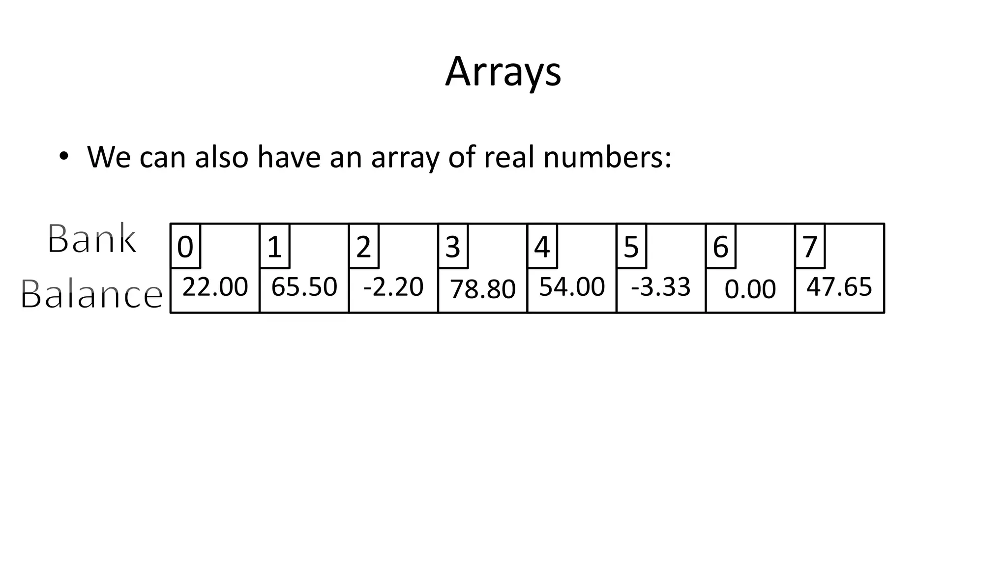
![• What if we wanted to check who has a balance less than zero :
PROGRAM LessThanZeroBalance:
integer ArraySize <- 8;
FOR N IN 0 TO ArraySize-1
DO IF BankBalance[N] < 0
THEN PRINT “User” N “is in debt”;
ENDIF;
ENDFOR;
END.
Arrays](https://image.slidesharecdn.com/completecourse-150726101701-lva1-app6892/75/A-complete-course-in-Program-Design-using-Pseudocode-353-2048.jpg)
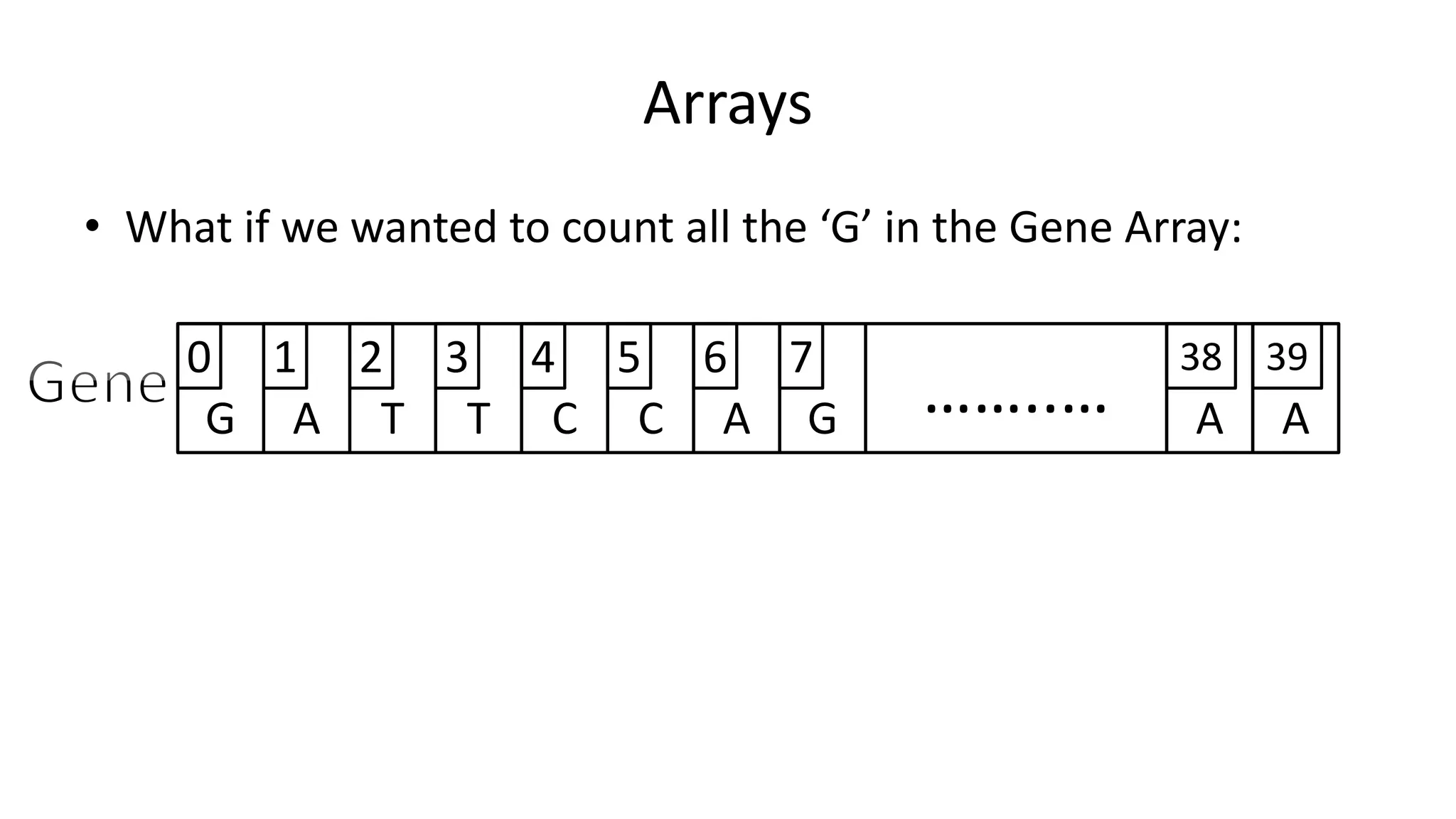
![• What if we wanted to count all the ‘G’ in the Gene Array:
PROGRAM AverageOfArray:
integer ArraySize <- 40;
integer G-Count <- 0;
FOR N IN 0 TO ArraySize-1
DO IF Gene[N] = ‘G’
THEN G-Count <- G-Count + 1;
ENDIF;
ENDFOR;
PRINT “The total G count is:” G-Count;
END.
Arrays](https://image.slidesharecdn.com/completecourse-150726101701-lva1-app6892/75/A-complete-course-in-Program-Design-using-Pseudocode-357-2048.jpg)
![• What if we wanted to count all the ‘A’ in the Gene Array:
PROGRAM AverageOfArray:
integer ArraySize <- 40;
integer A-Count <- 0;
FOR N IN 0 TO ArraySize-1
DO IF Gene[N] = ‘A’
THEN A-Count <- A-Count + 1;
ENDIF;
ENDFOR;
PRINT “The total A count is:” A-Count;
END.
Arrays](https://image.slidesharecdn.com/completecourse-150726101701-lva1-app6892/75/A-complete-course-in-Program-Design-using-Pseudocode-358-2048.jpg)


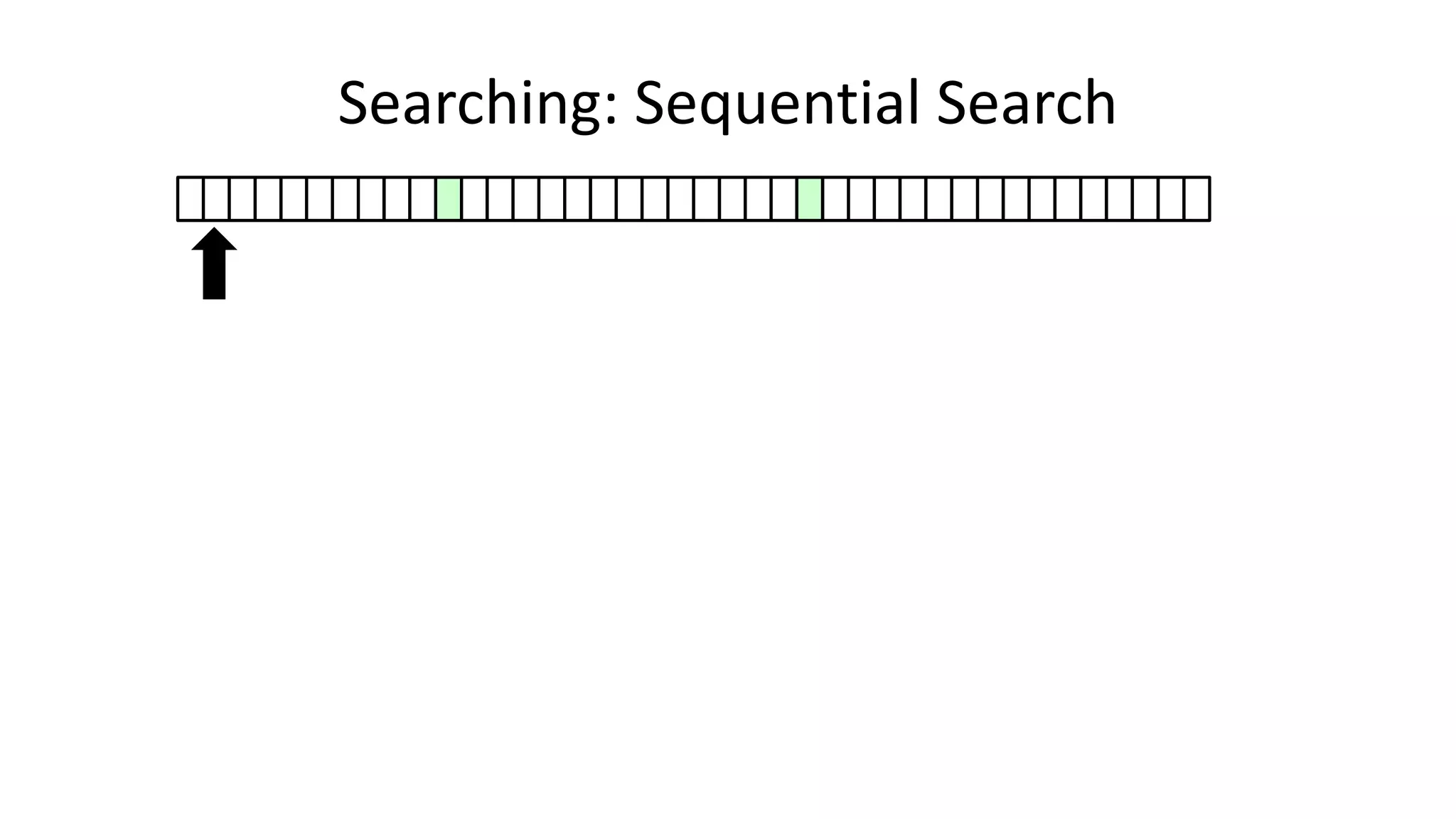
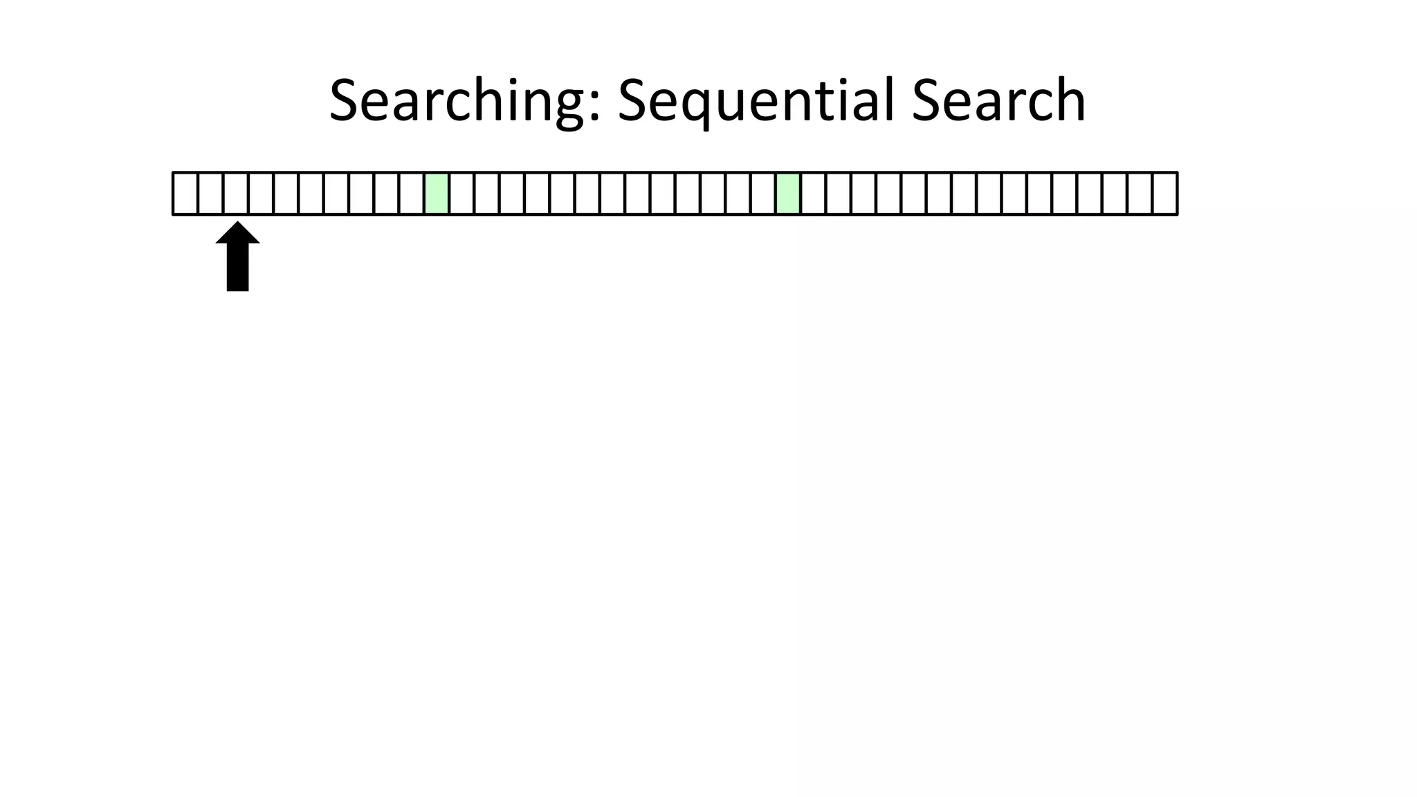
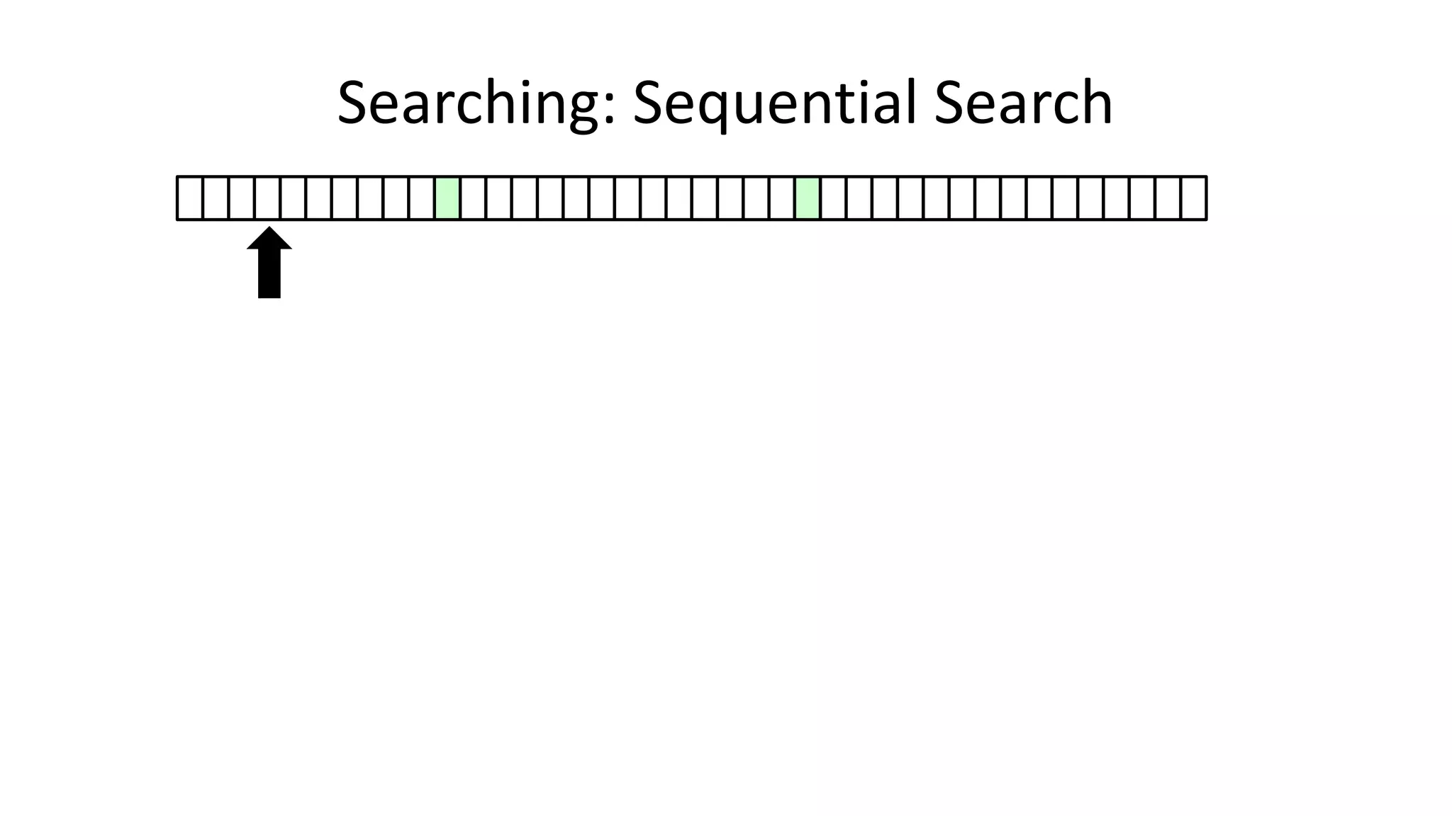
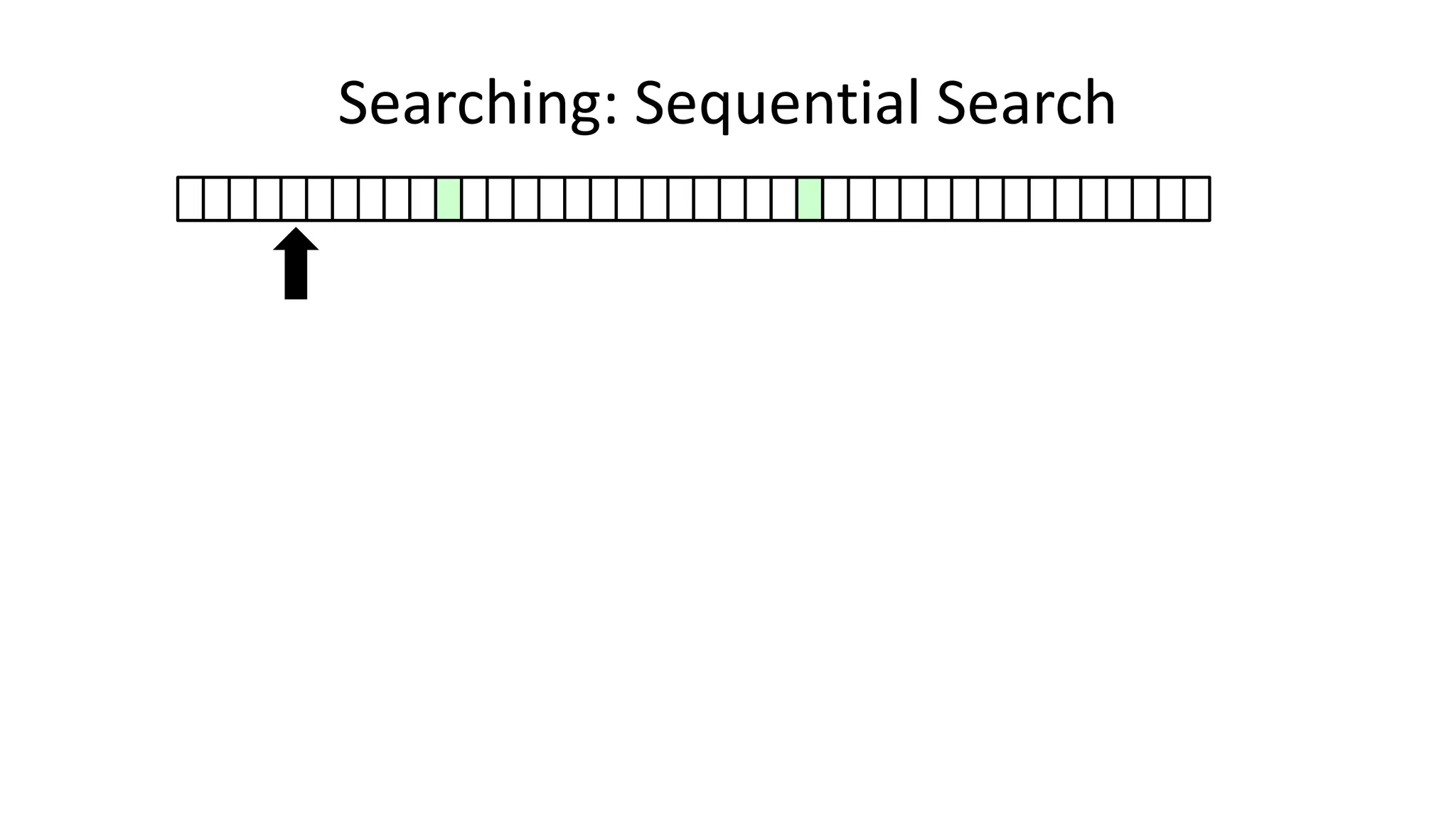
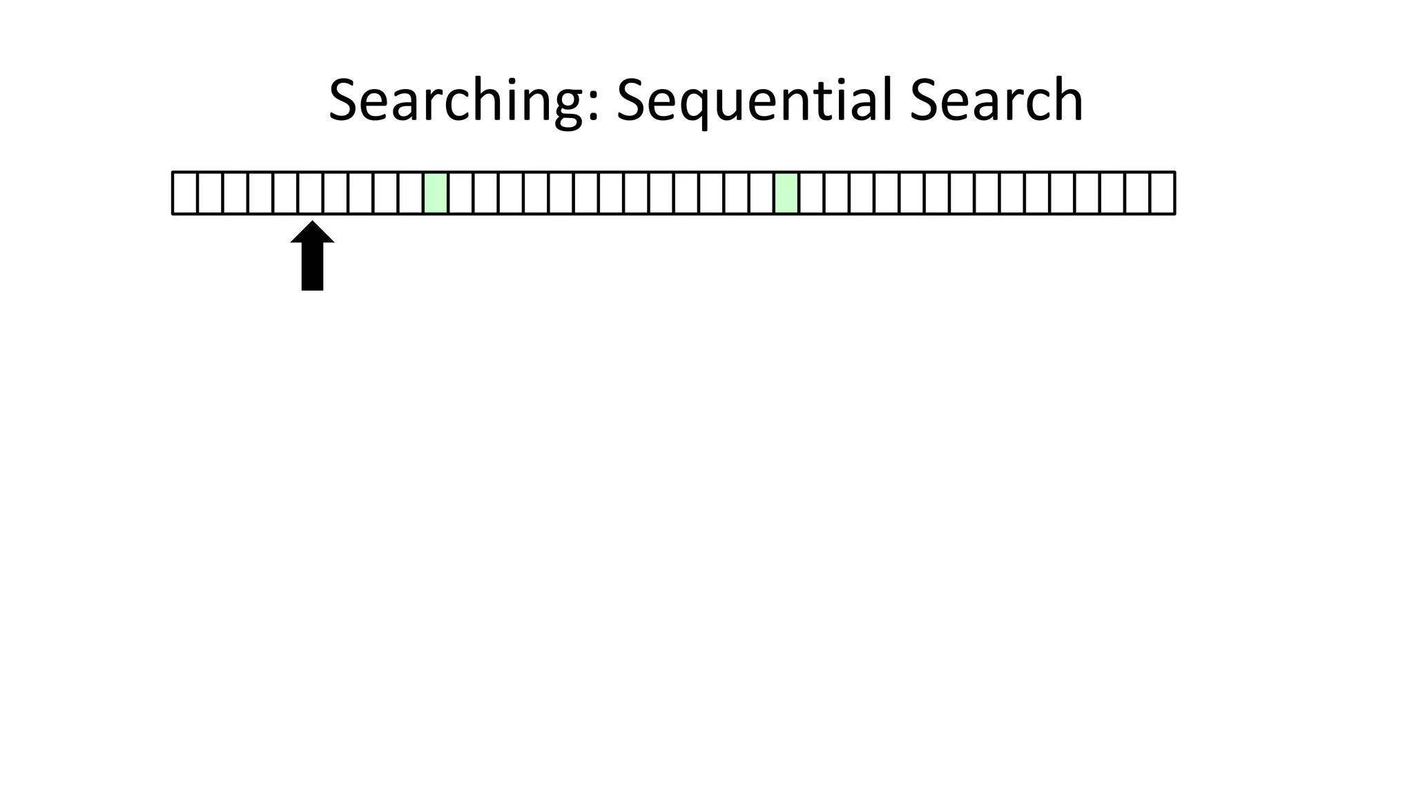
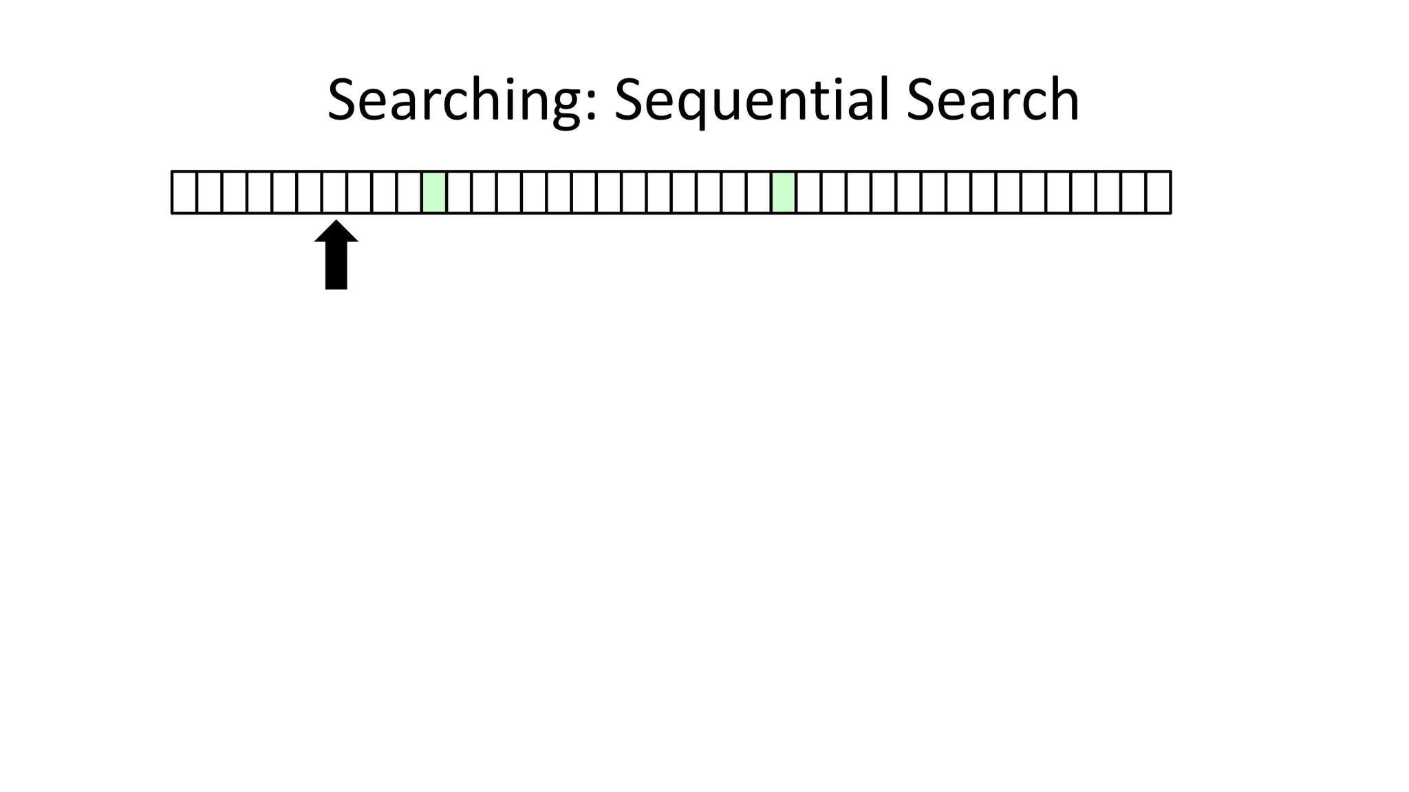
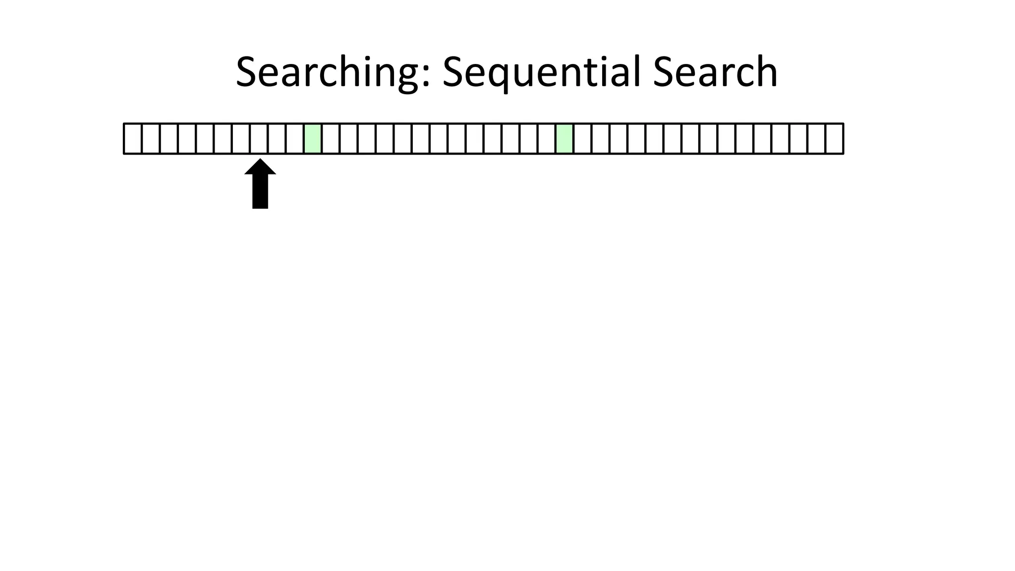
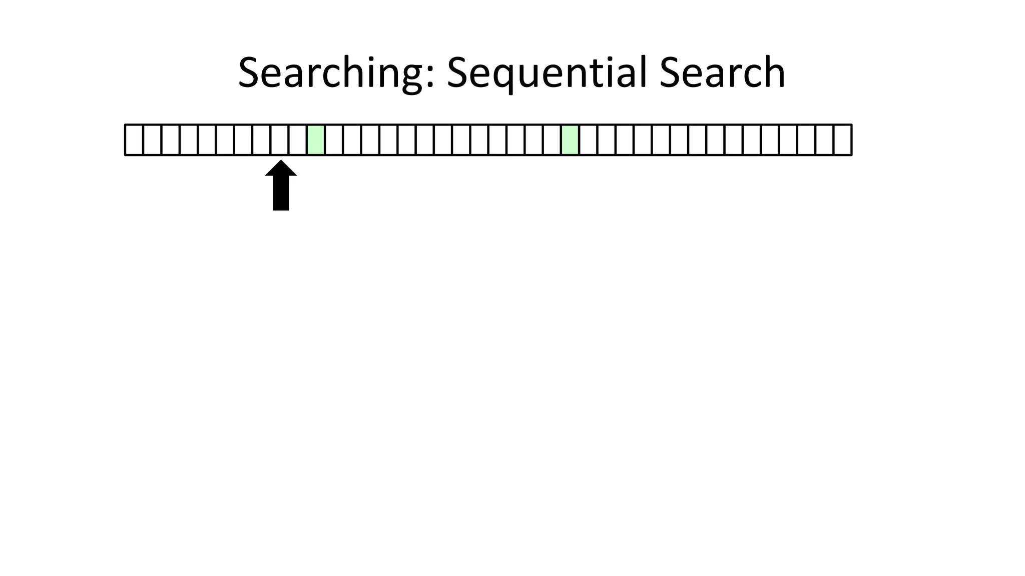
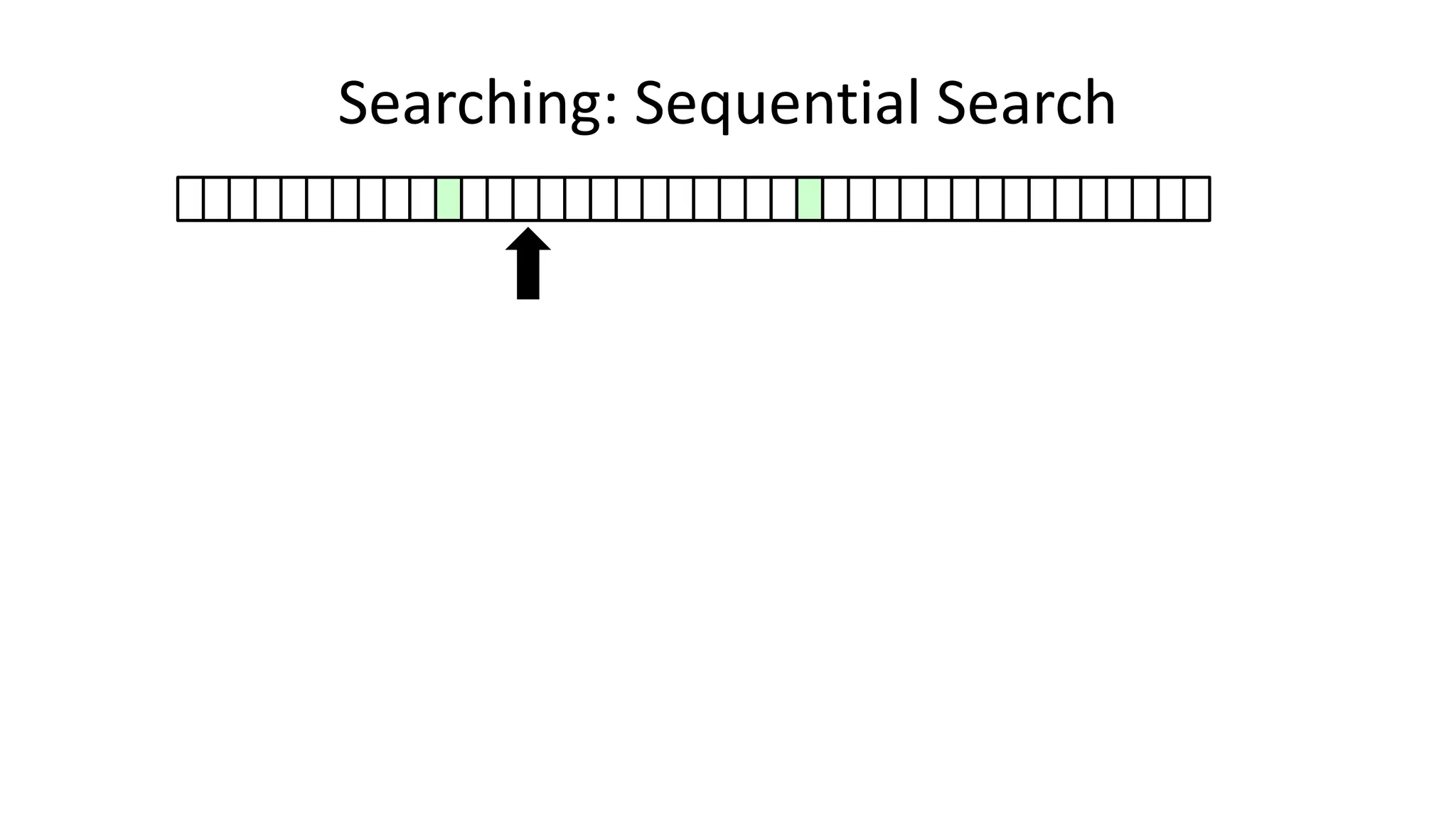
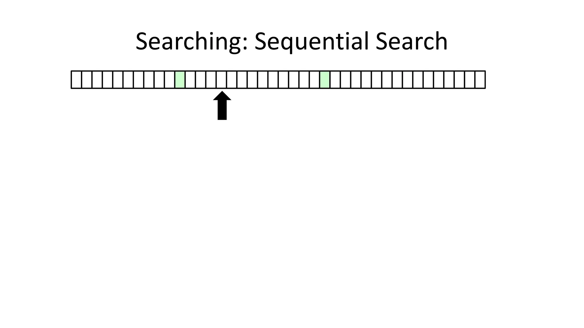
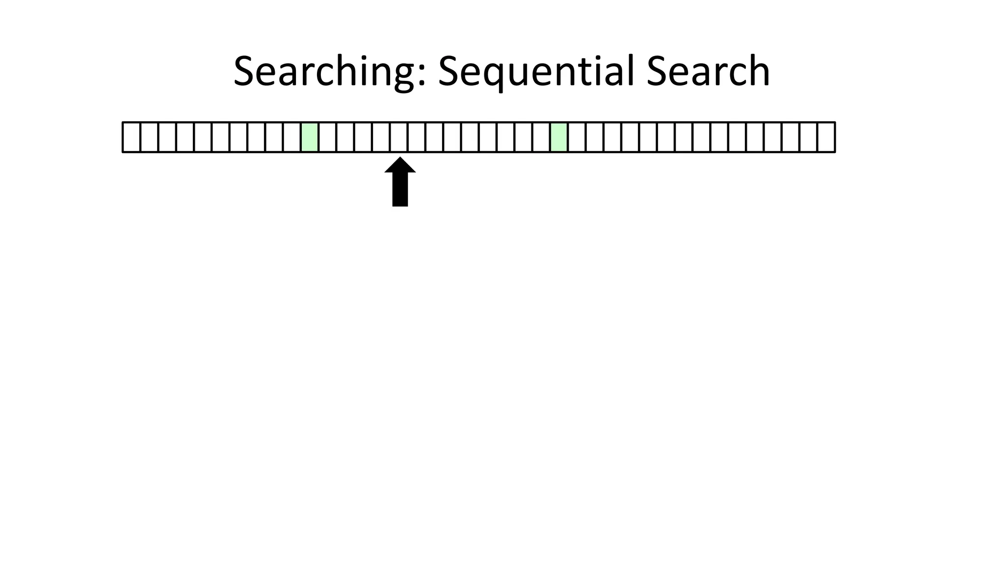
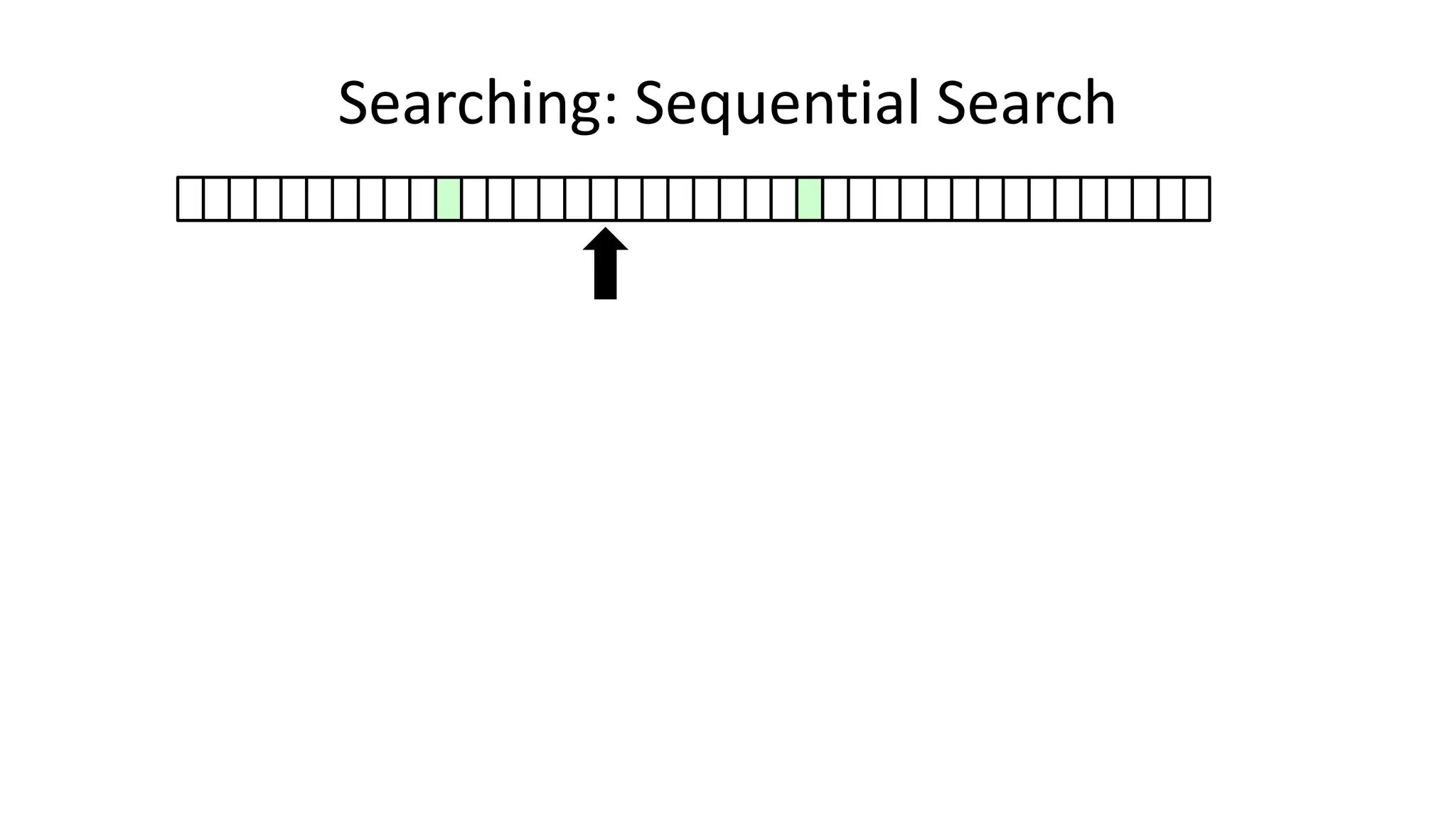

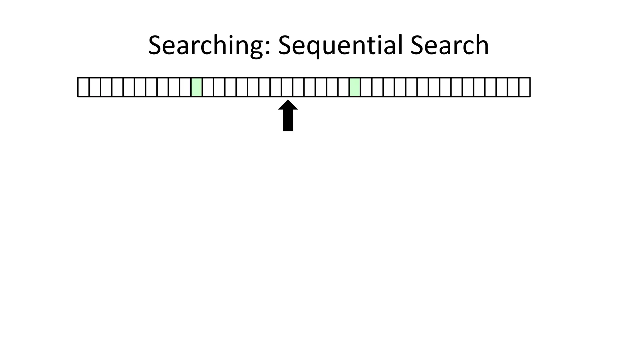
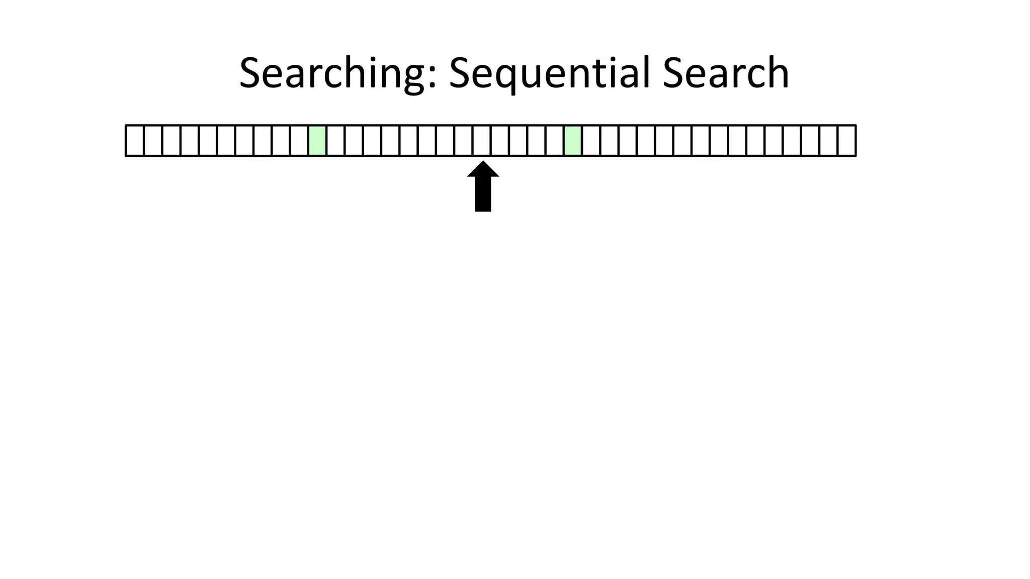
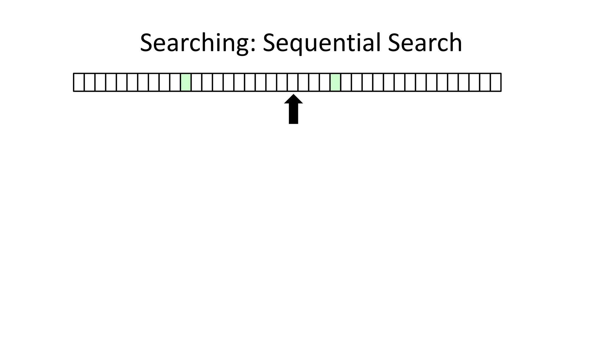
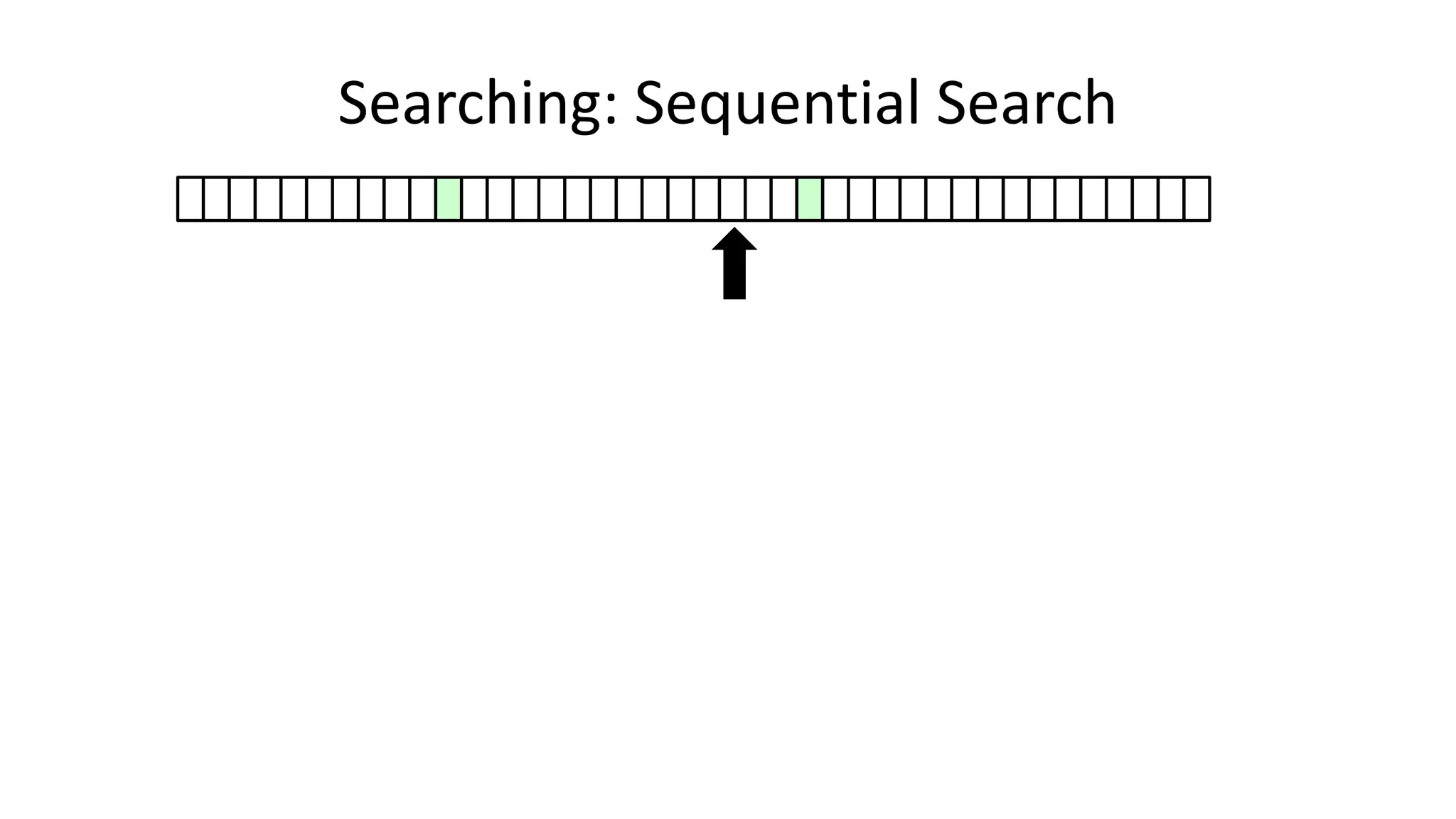

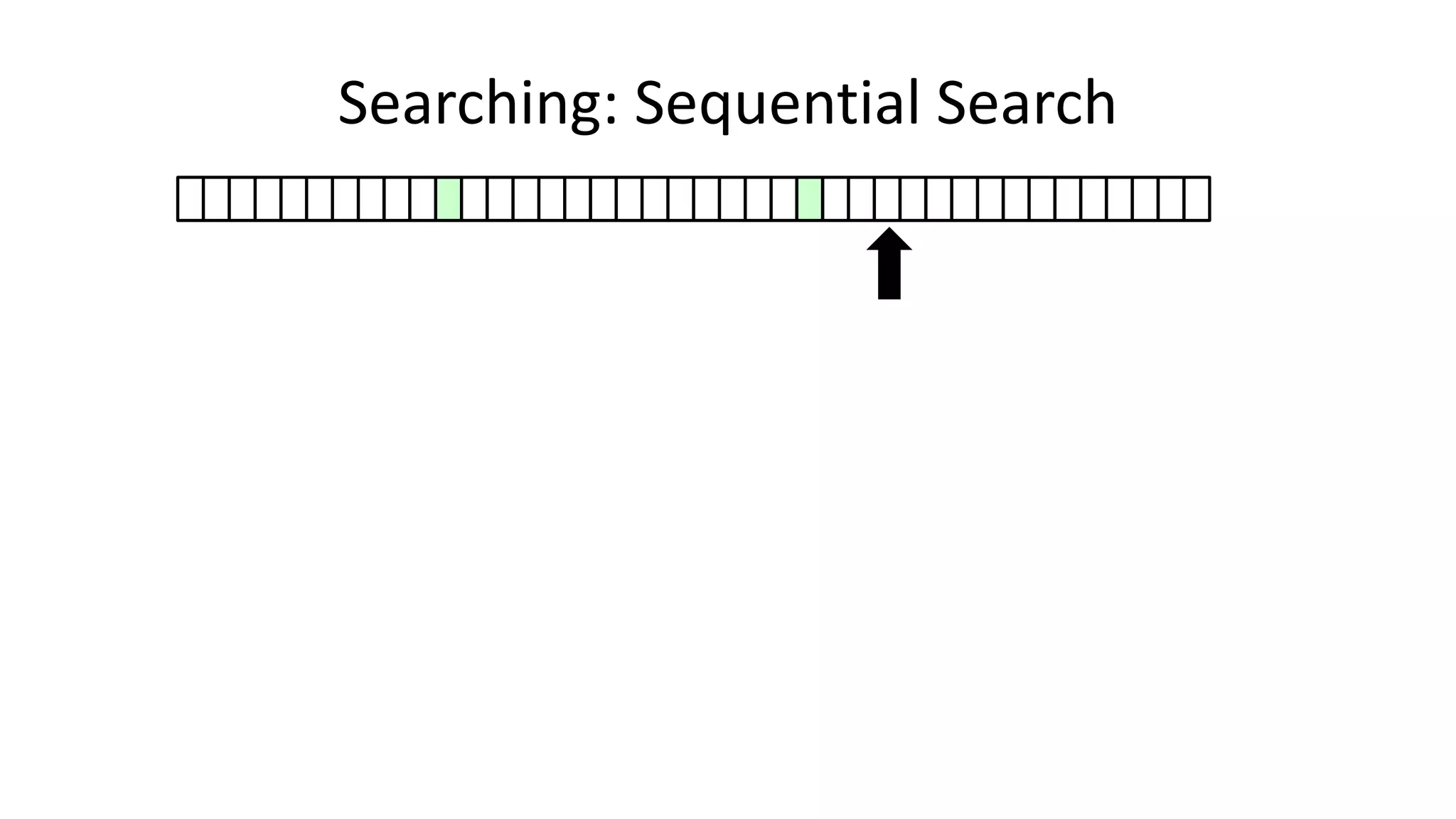
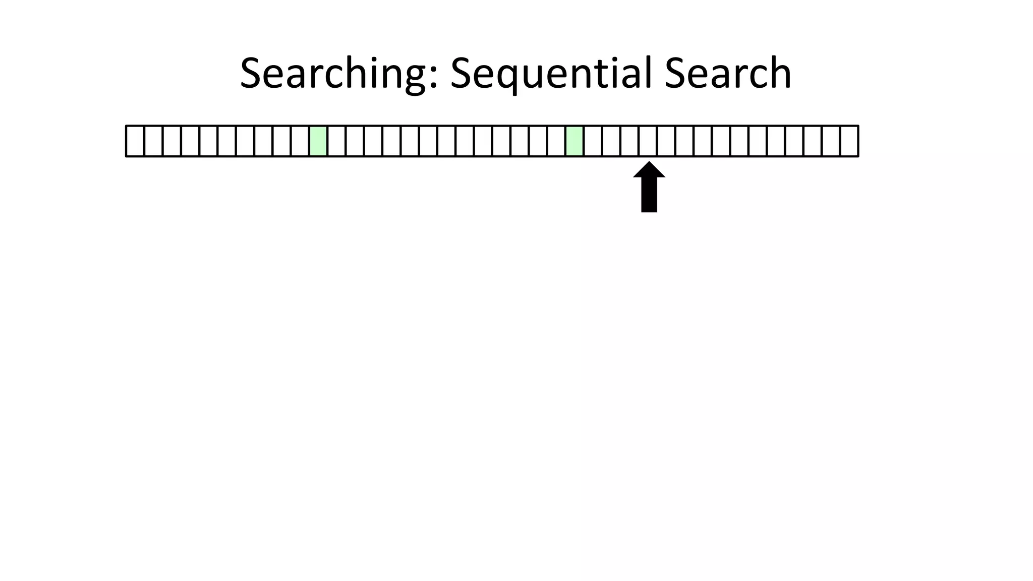

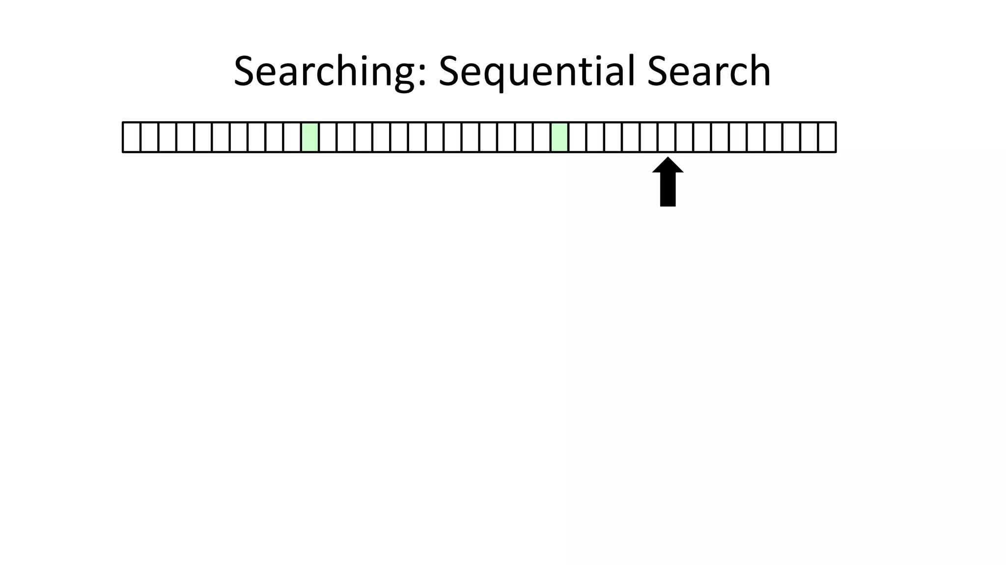
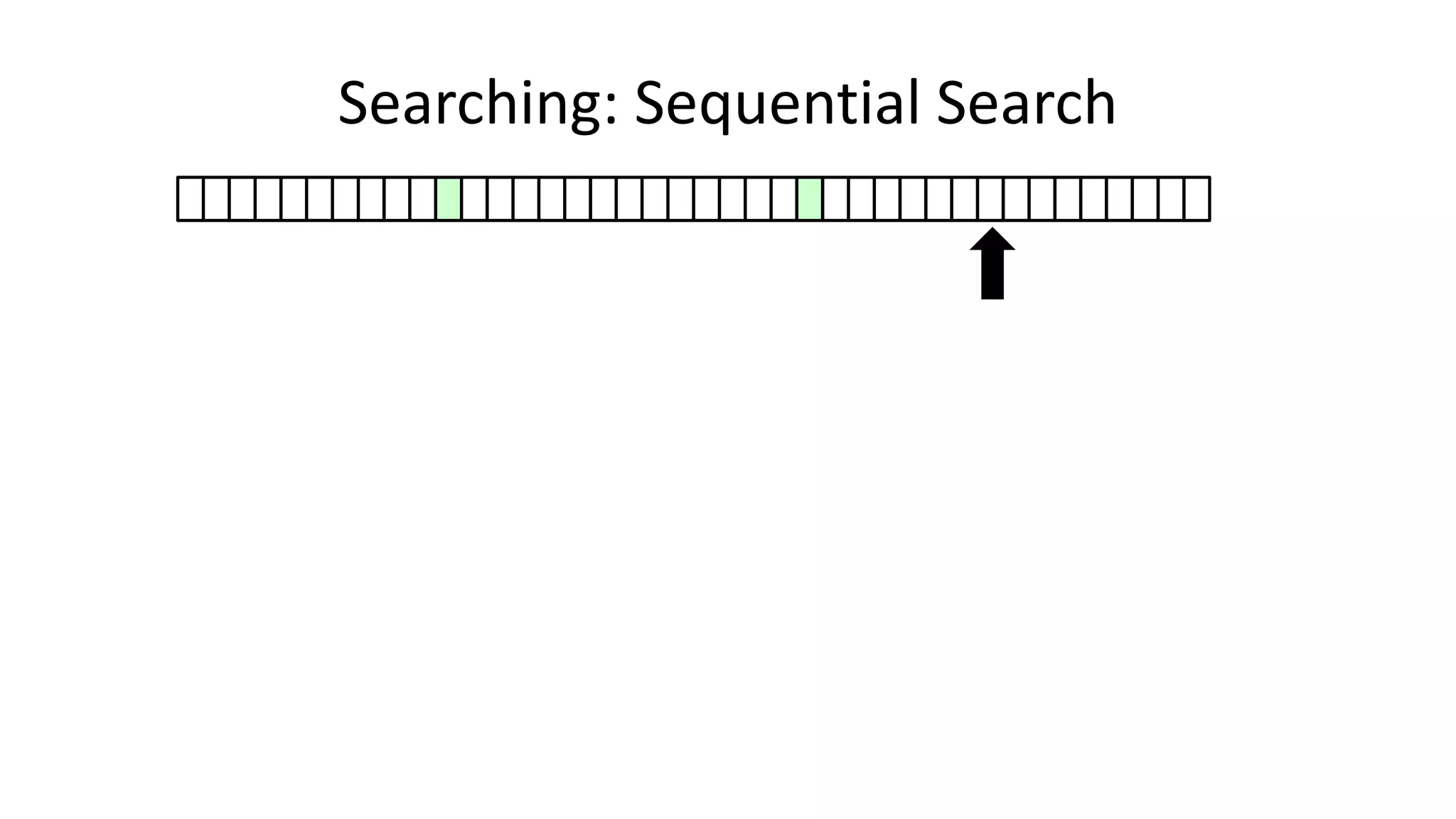
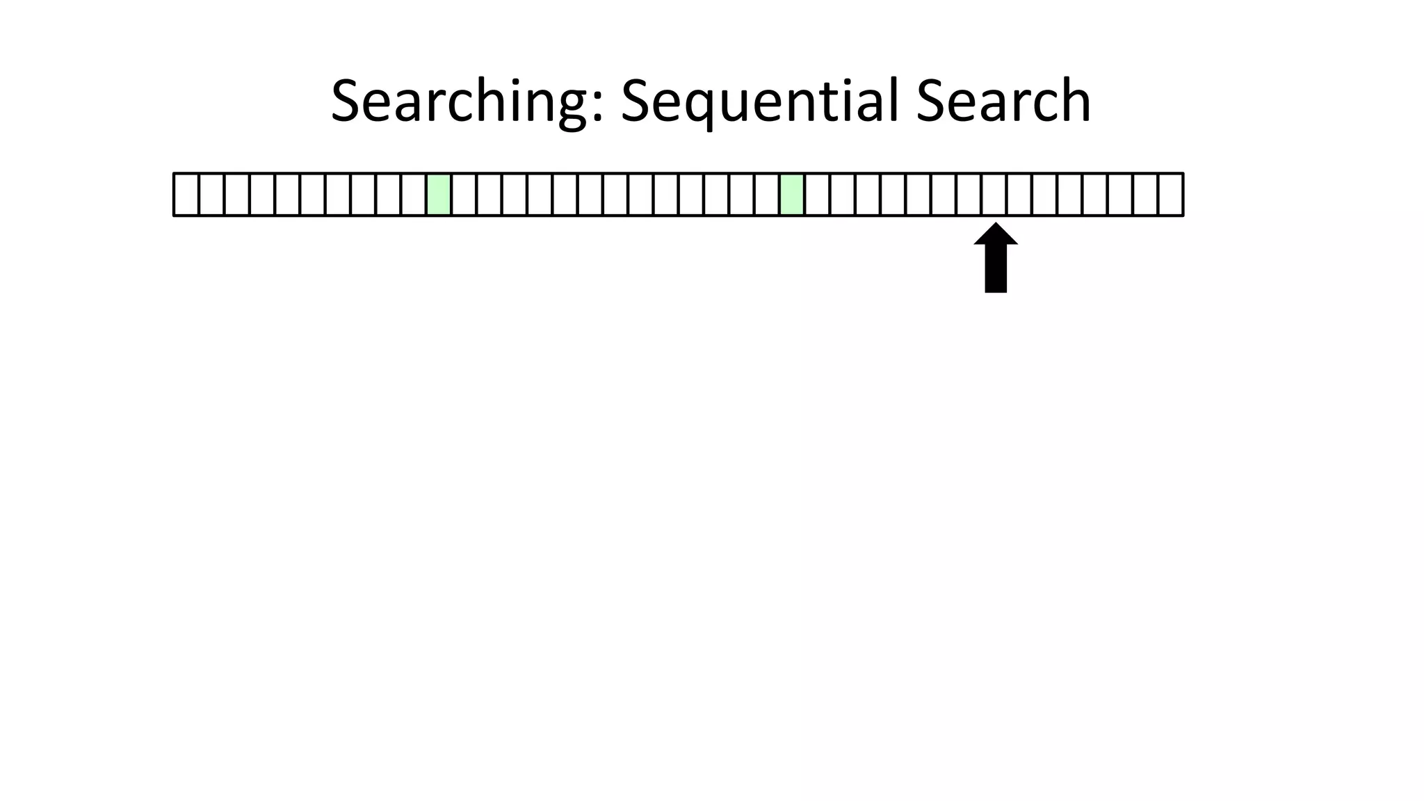
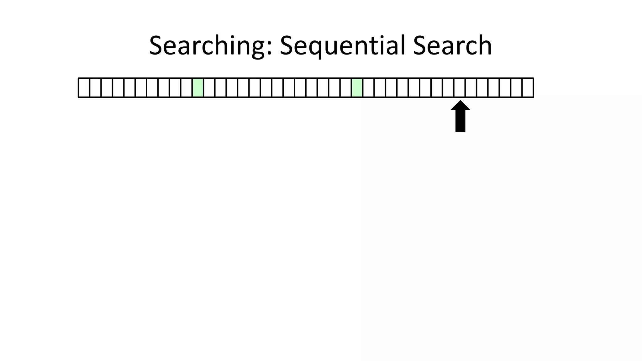
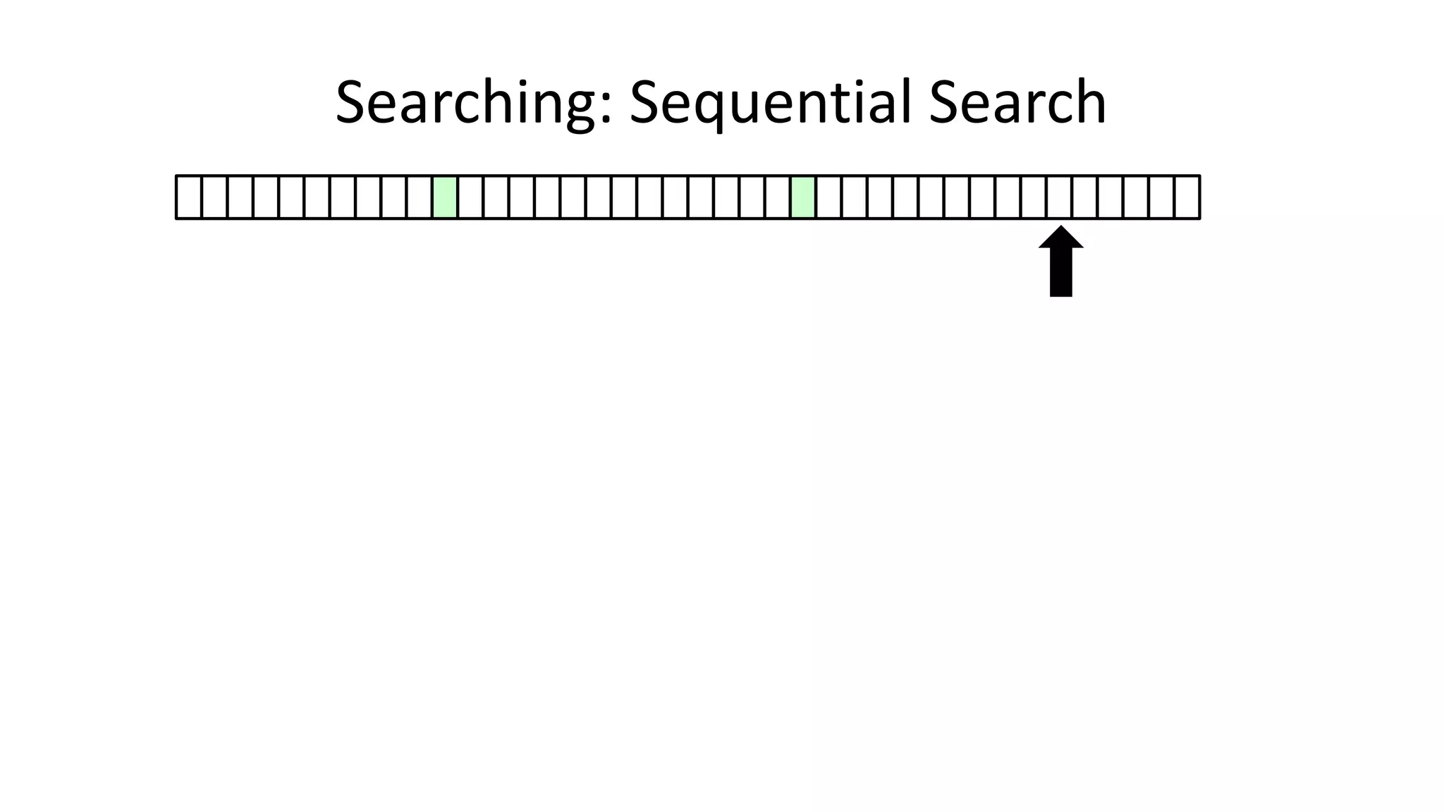
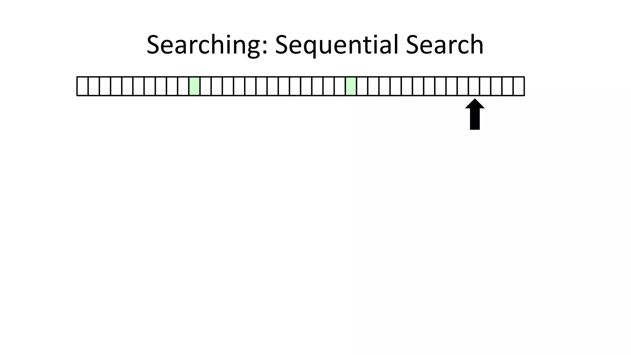
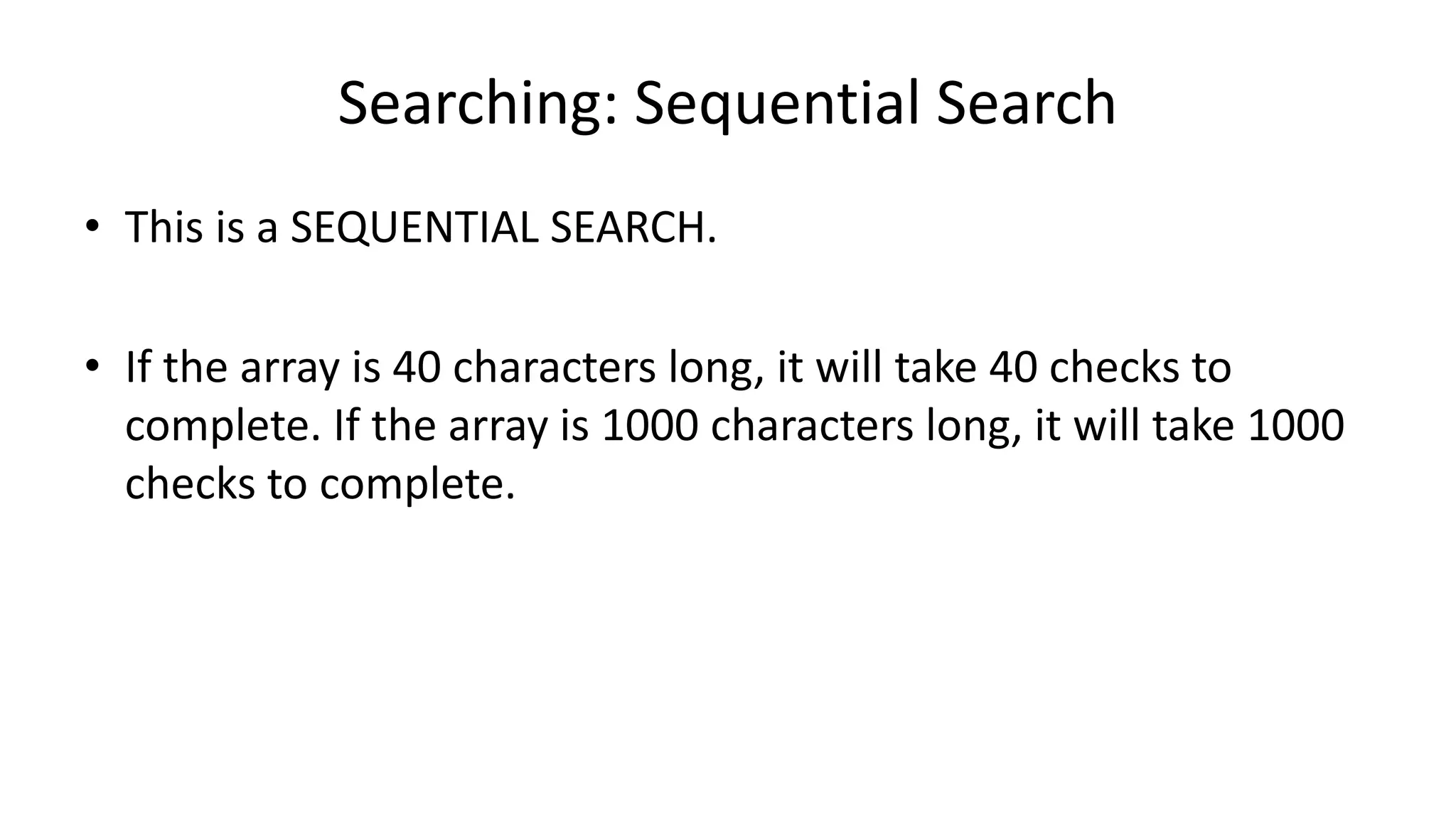
![• Here’s how we could do it:
PROGRAM SequentialSearch:
integer SearchValue <- 18;
integer ArraySize <- 40;
FOR N IN 0 TO ArraySize-1
DO IF Age[N] = SearchValue
THEN PRINT “User “ N “is 18”;
ENDIF;
ENDFOR;
END.
Searching: Sequential Search](https://image.slidesharecdn.com/completecourse-150726101701-lva1-app6892/75/A-complete-course-in-Program-Design-using-Pseudocode-420-2048.jpg)

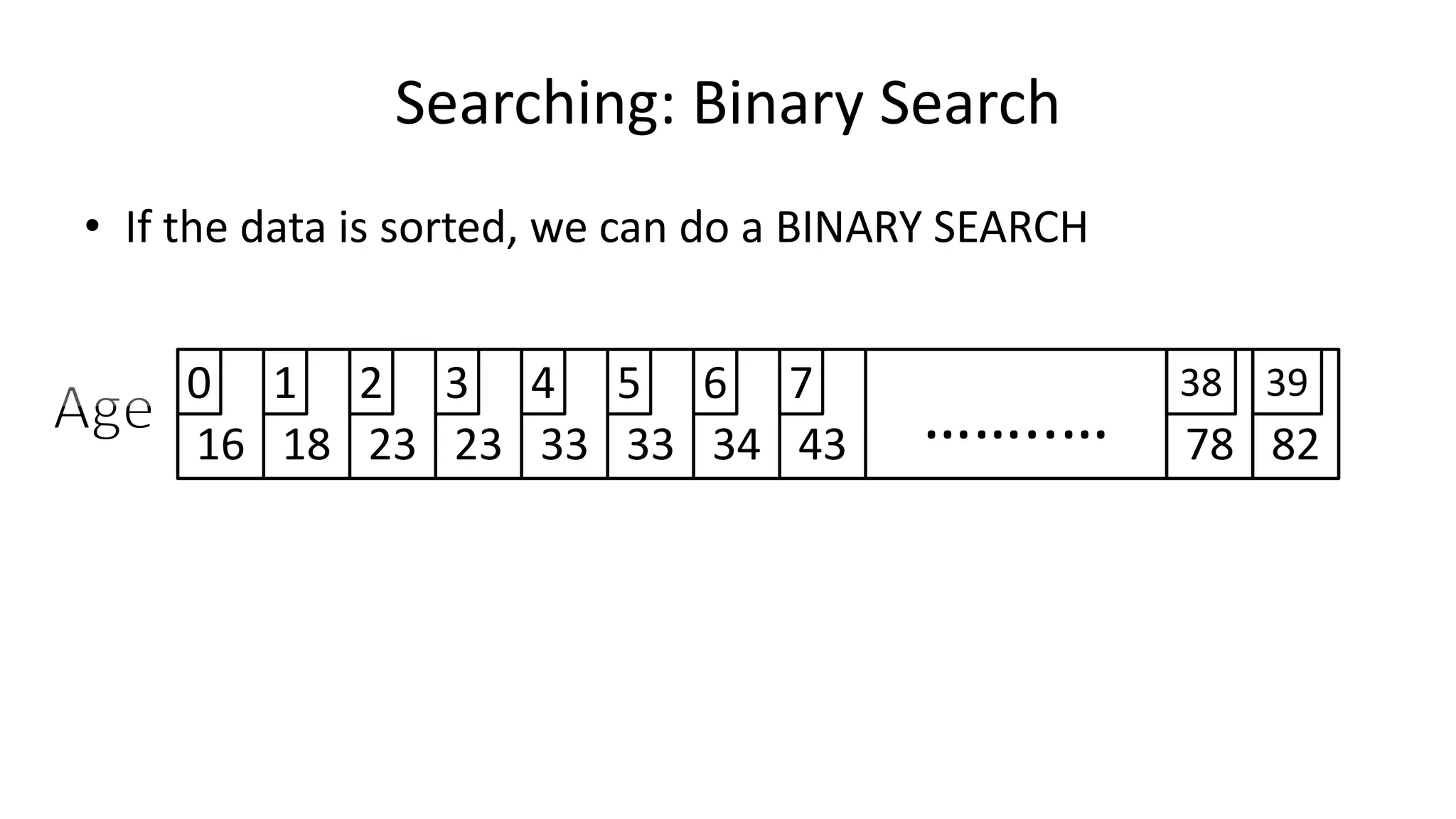


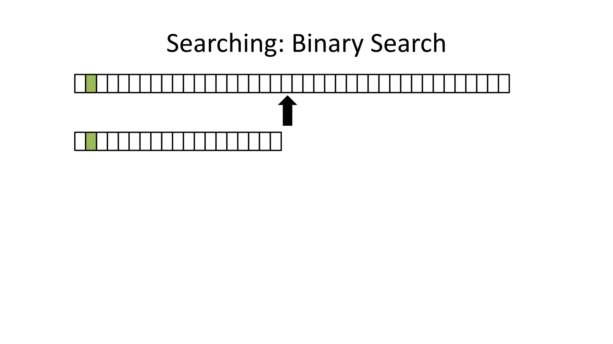
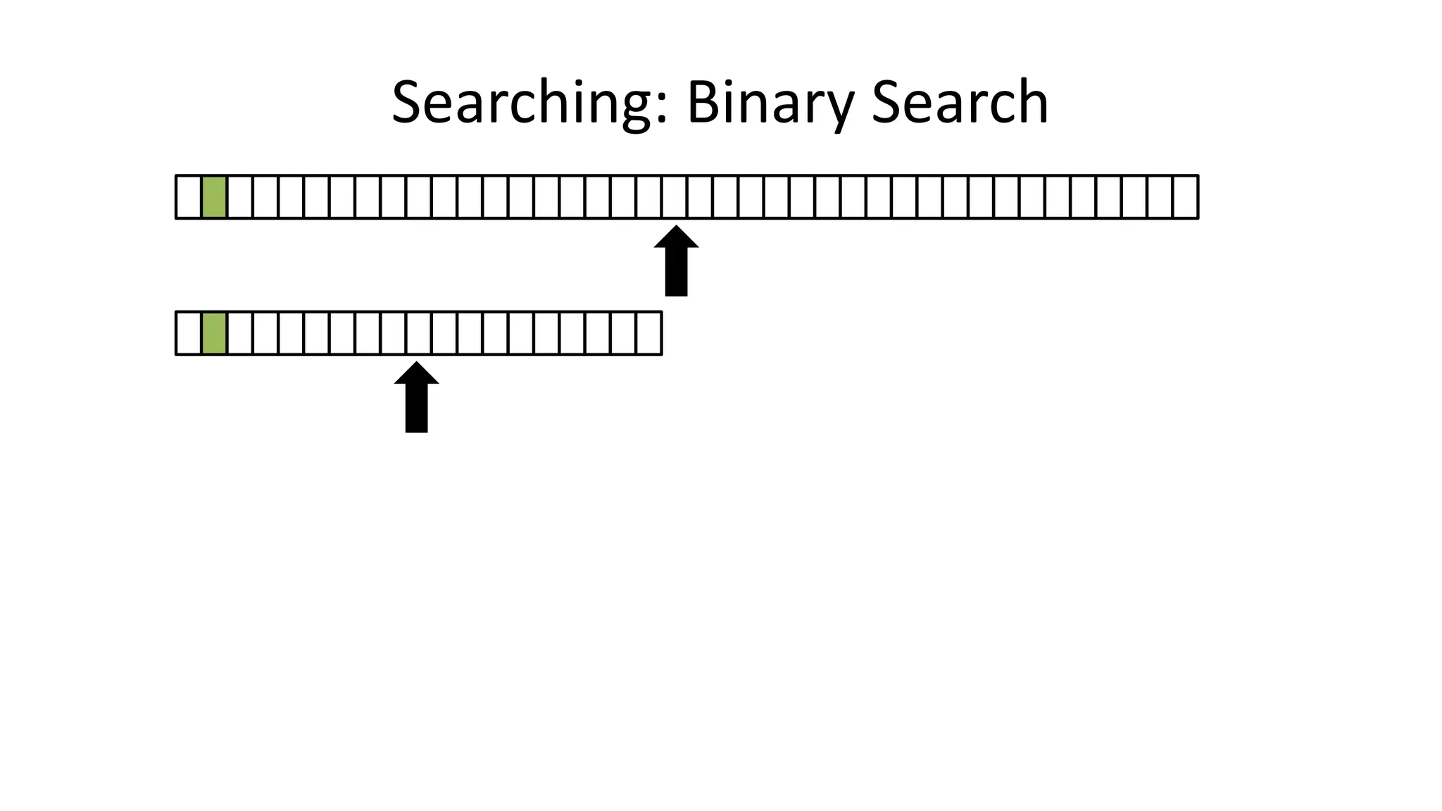
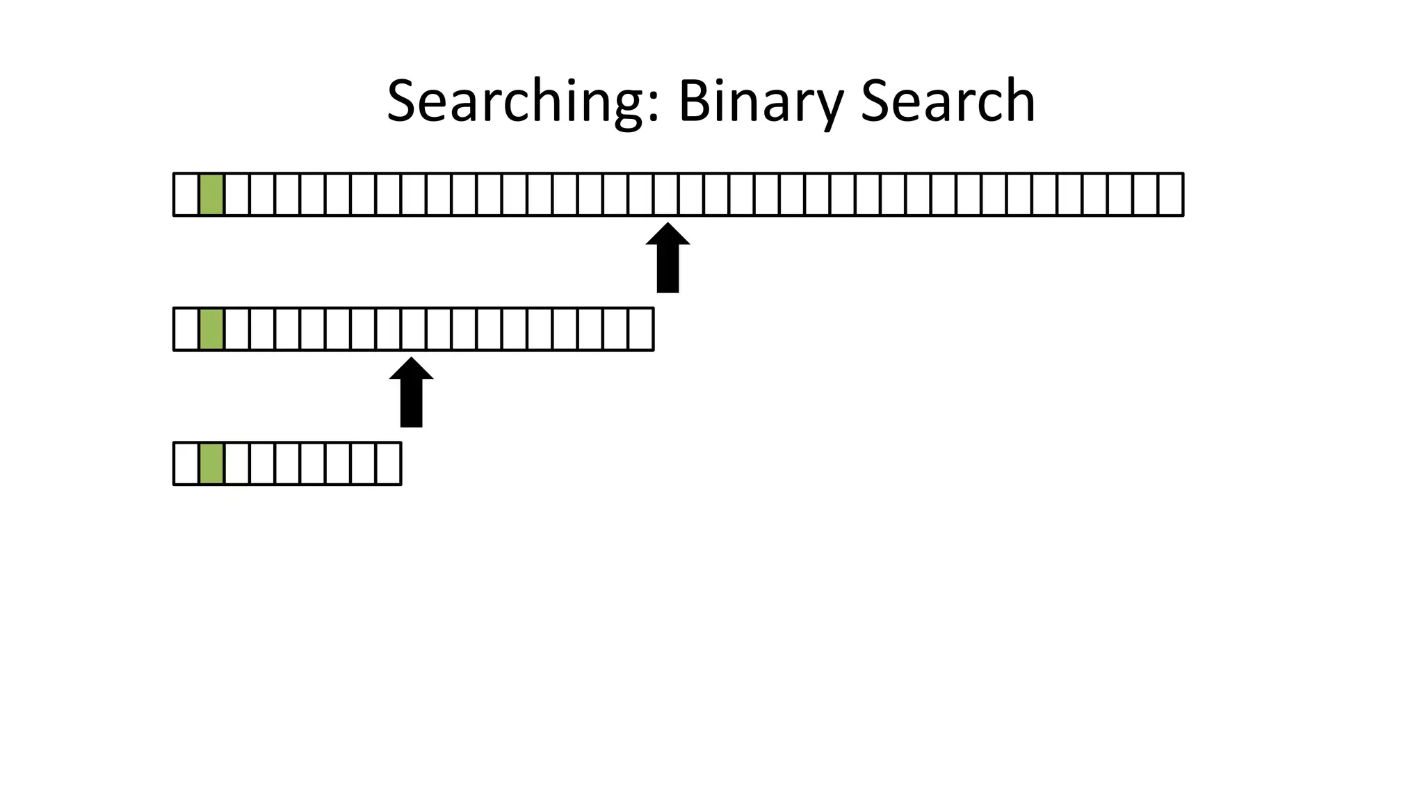
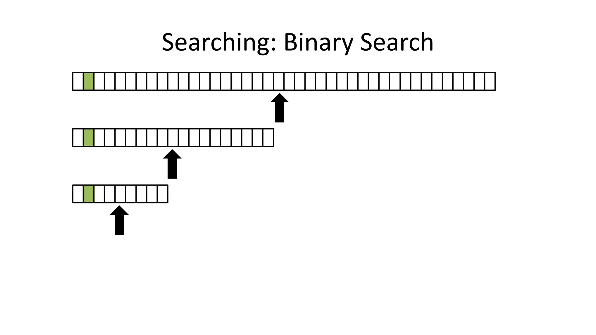
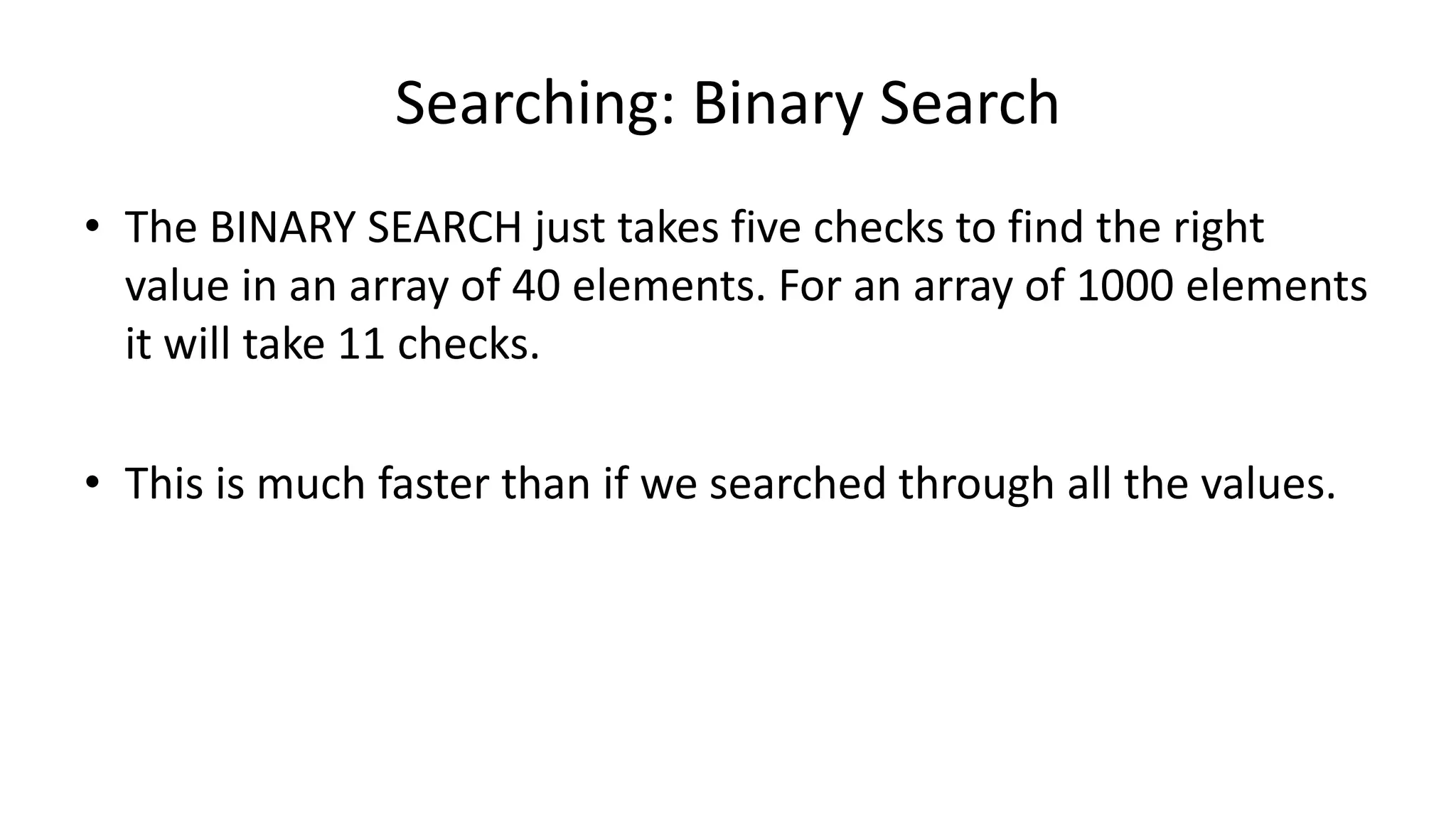
![• If the data is sorted, we can do a BINARY SEARCH
PROGRAM BinarySearch:
integer First <- 0;
integer Last <- 40;
boolean IsFound <- FALSE;
WHILE First <= Last AND IsFound = FALSE
DO Index = (First + Last)/2;
IF Age[Index] = SearchValue
THEN IsFound <- TRUE;
ELSE IF Age[Index] > SearchValue
THEN Last <- Index-1;
ELSE First <- Index+1;
ENDIF;
ENDIF;
ENDWHILE;
END.
Searching: Binary Search](https://image.slidesharecdn.com/completecourse-150726101701-lva1-app6892/75/A-complete-course-in-Program-Design-using-Pseudocode-437-2048.jpg)

![• Here’s how we could do it:
PROGRAM MinimumValue:
integer ArraySize <- 8;
MinValSoFar <- Age[0];
FOR N IN 1 TO ArraySize-1
DO IF MinValSoFar > Age[N]
THEN MinValSoFar <- Age[N];
ENDIF;
ENDFOR;
PRINT MinValSoFar;
END.
Minimum Value in Array](https://image.slidesharecdn.com/completecourse-150726101701-lva1-app6892/75/A-complete-course-in-Program-Design-using-Pseudocode-441-2048.jpg)
![• Here’s how we could do it:
PROGRAM MaximumValue:
integer ArraySize <- 8;
MaxValSoFar <- Age[0];
FOR N IN 1 TO ArraySize-1
DO IF MaxValSoFar < Age[N]
THEN MaxValSoFar <- Age[N];
ENDIF;
ENDFOR;
PRINT MaxValSoFar;
END.
Maximum Value in Array](https://image.slidesharecdn.com/completecourse-150726101701-lva1-app6892/75/A-complete-course-in-Program-Design-using-Pseudocode-443-2048.jpg)
![• Here’s how we could do it:
PROGRAM AverageValue:
integer ArraySize <- 8;
Integer Total <- 0;
FOR N IN 1 TO ArraySize-1
DO Total <- Total + Age[N];
ENDFOR;
PRINT Total/ArraySize;
END.
Average Value in Array](https://image.slidesharecdn.com/completecourse-150726101701-lva1-app6892/75/A-complete-course-in-Program-Design-using-Pseudocode-445-2048.jpg)
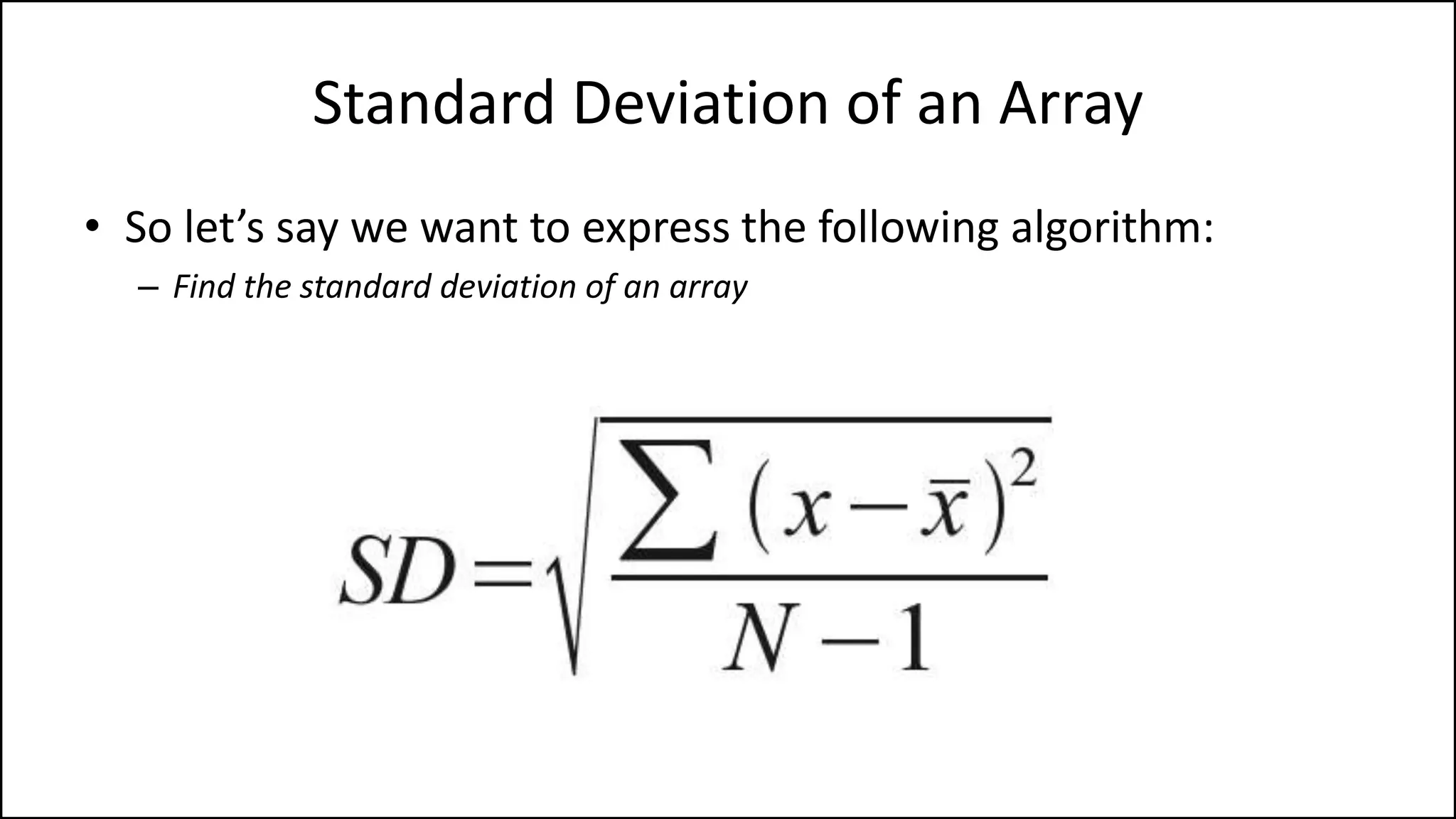
![• First Draft
PROGRAM StandardDeviationValue:
integer ArraySize <- 8;
GET AVERAGE OF ARRAY;
TotalSDNum <- 0;
FOR N IN 0 TO ArraySize-1
DO SDNum <-(Age[N]-ArrayAvg)*(Age[N]-ArrayAvg)
TotalSDNum <- TotalSDNum + SDNum;
ENDFOR;
Print SquareRoot(TotalSDNum/ArraySize-1);
END.
Standard Deviation of an Array](https://image.slidesharecdn.com/completecourse-150726101701-lva1-app6892/75/A-complete-course-in-Program-Design-using-Pseudocode-448-2048.jpg)
![• Here’s the final version:
PROGRAM StandardDeviationValue:
integer ArraySize <- 8;
Integer TotalAvg <- 0;
FOR N IN 1 TO ArraySize-1
DO TotalAvg <- TotalAvg + Age[N];
ENDFOR;
AverageValue <- TotalAvg/ArraySize;
TotalSDNum <- 0;
FOR N IN 0 TO ArraySize-1
DO SDNum <-(Age[N]-AverageValue)*(Age[N]- AverageValue)
TotalSDNum <- TotalSDNum + SDNum;
ENDFOR;
Print SquareRoot(TotalSDNum/ArraySize-1);
END.
Standard Deviation of an Array](https://image.slidesharecdn.com/completecourse-150726101701-lva1-app6892/75/A-complete-course-in-Program-Design-using-Pseudocode-449-2048.jpg)


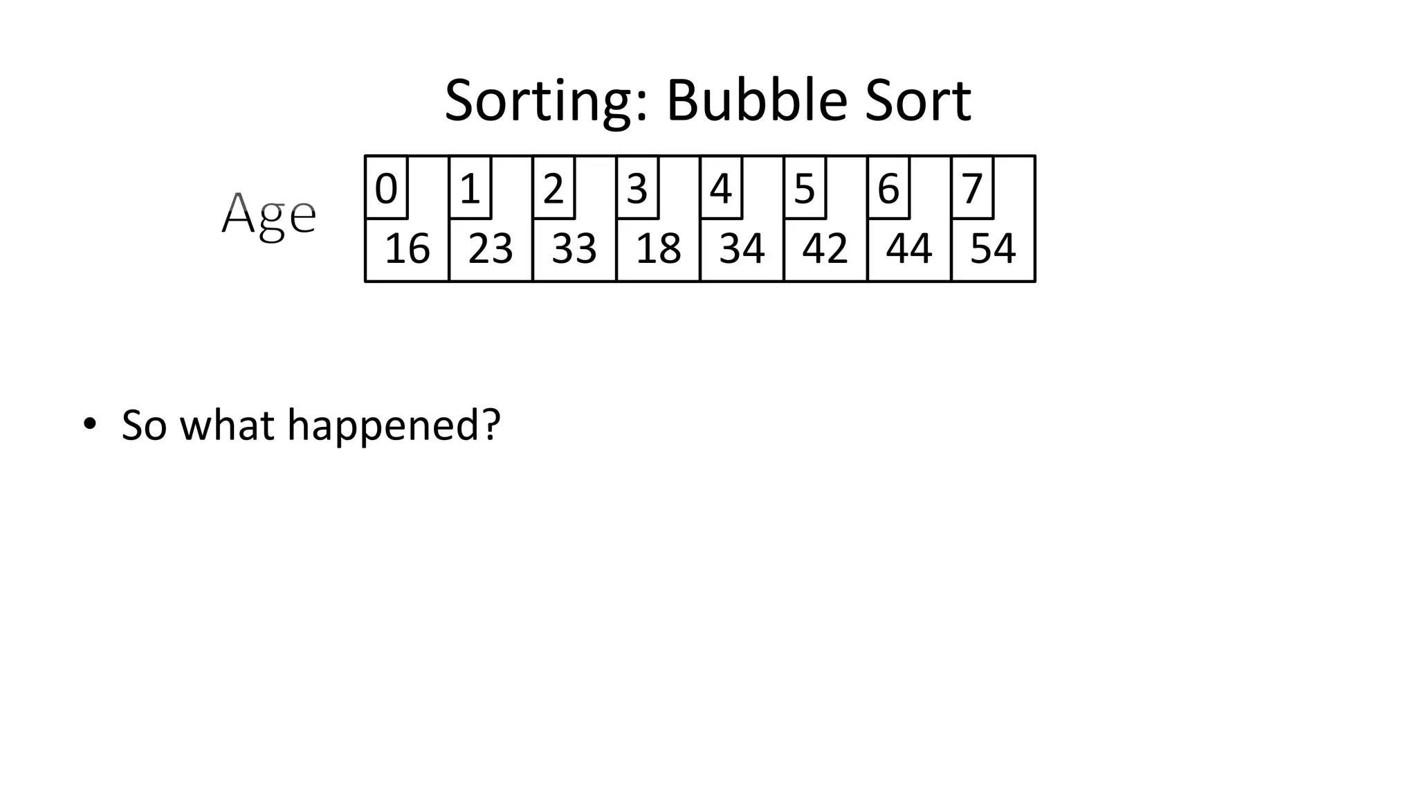
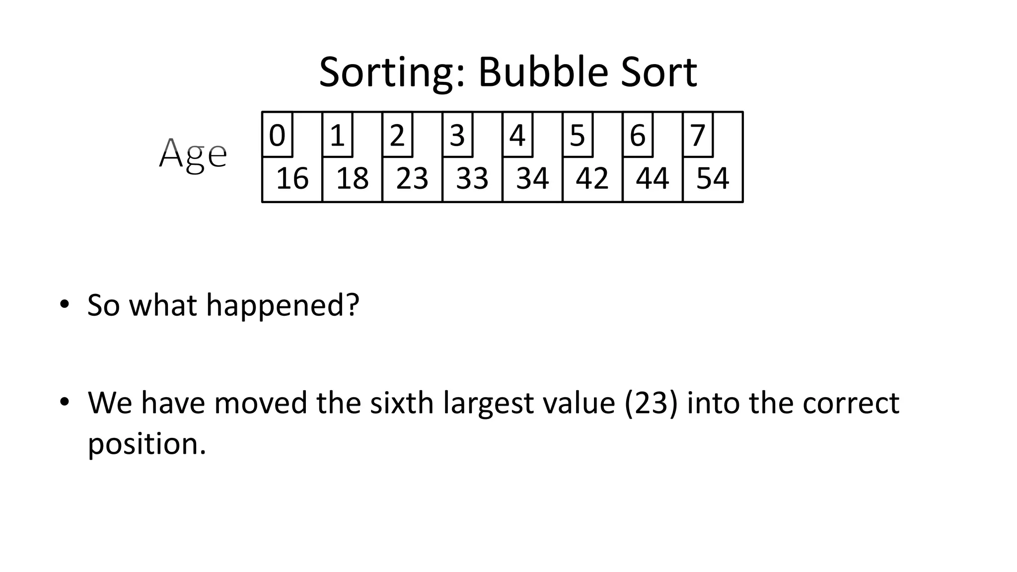
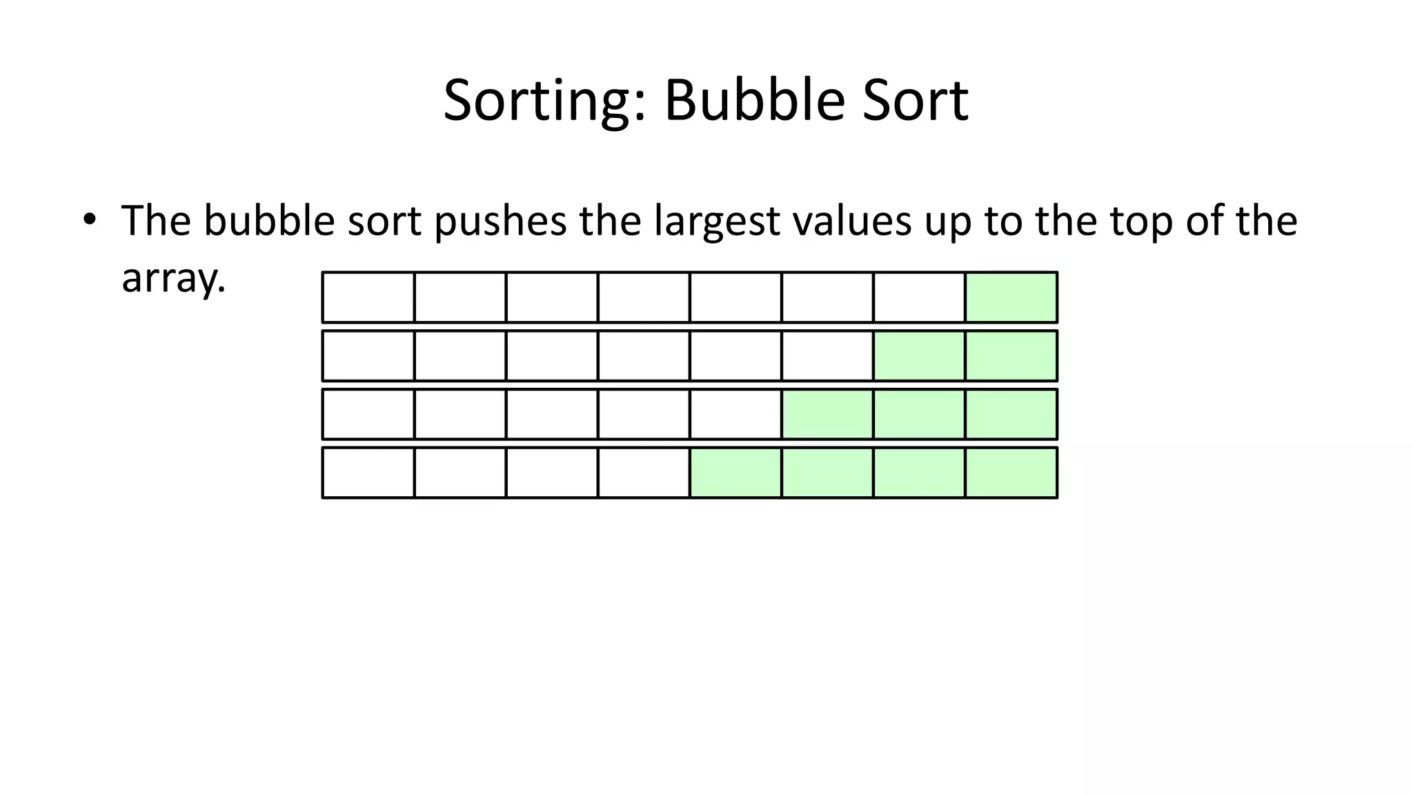
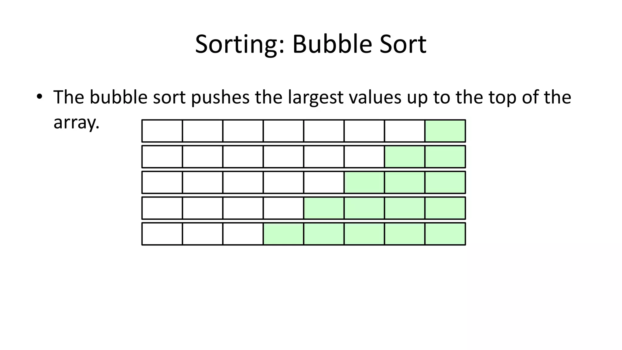
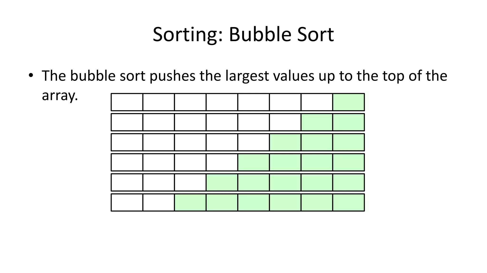
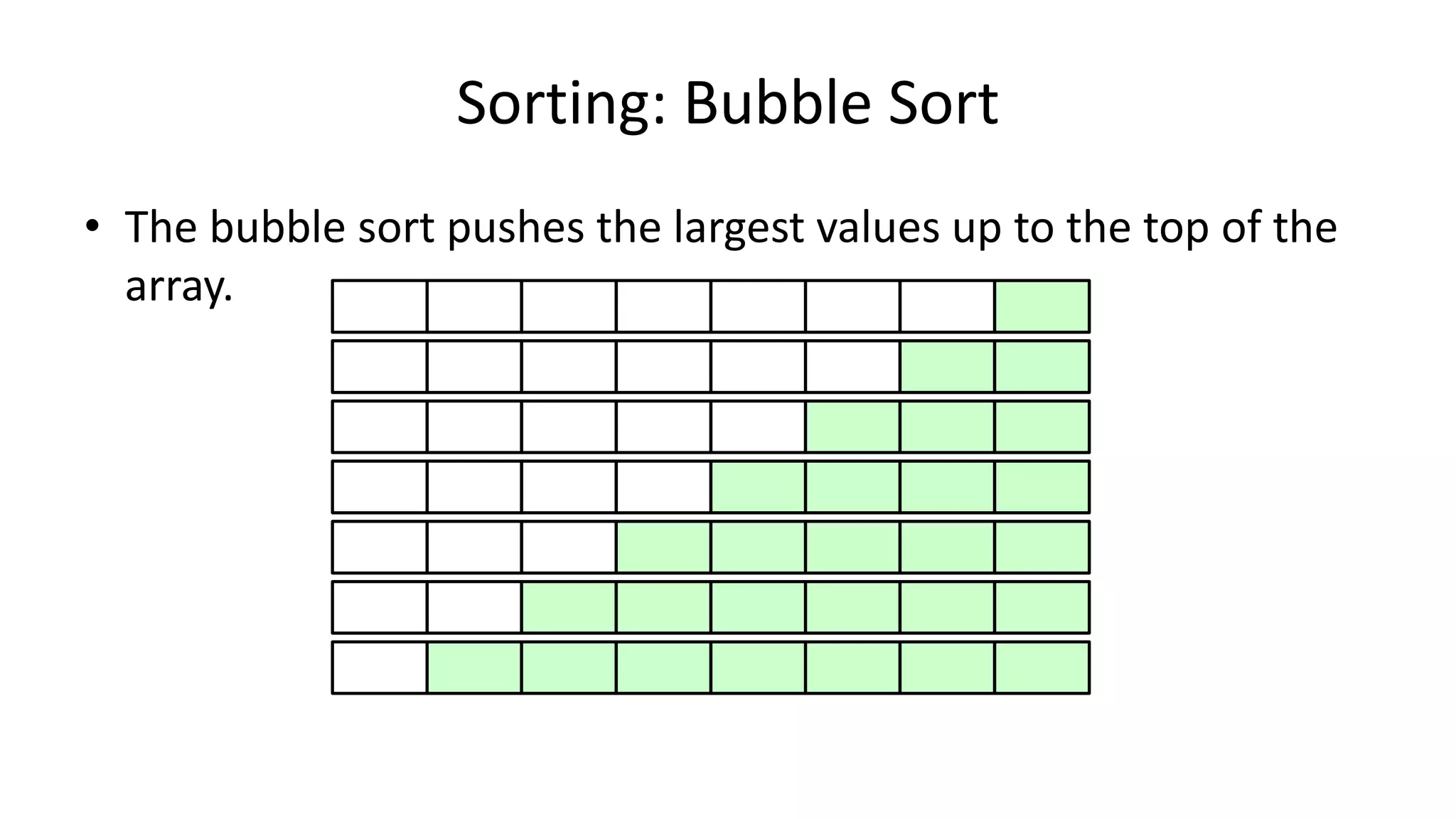
![• Lets look at the swapping bit
– if I wanted to swap two values, the following won’t work:
Age[0] <- Age[1];
Age[1] <- Age[0];
– Why not?
Sorting: Bubble Sort](https://image.slidesharecdn.com/completecourse-150726101701-lva1-app6892/75/A-complete-course-in-Program-Design-using-Pseudocode-460-2048.jpg)
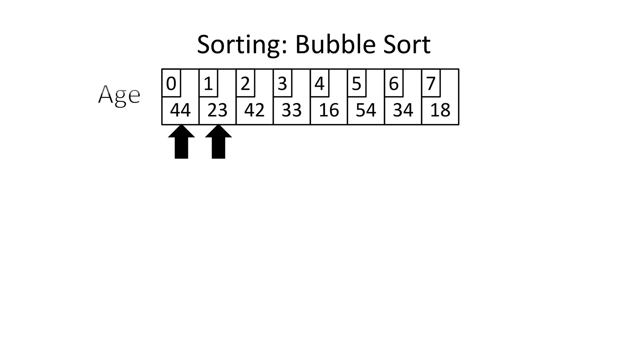
![• Lets assume Age[0]=44, and Age[1]=23, if we do the following:
Age[0] <- Age[1];
Age[1] <- Age[0];
– What happens is:
Age[0] <- Age[1];
Age[1] <- Age[0];
Sorting: Bubble Sort](https://image.slidesharecdn.com/completecourse-150726101701-lva1-app6892/75/A-complete-course-in-Program-Design-using-Pseudocode-461-2048.jpg)
![• Lets assume Age[0]=44, and Age[1]=23, if we do the following:
Age[0] <- Age[1];
Age[1] <- Age[0];
– What happens is:
Age[0] <- Age[1];
Age[1] <- Age[0];
Sorting: Bubble Sort
23](https://image.slidesharecdn.com/completecourse-150726101701-lva1-app6892/75/A-complete-course-in-Program-Design-using-Pseudocode-462-2048.jpg)
![• Lets assume Age[0]=44, and Age[1]=23, if we do the following:
Age[0] <- Age[1];
Age[1] <- Age[0];
– What happens is:
Age[0] <- Age[1];
Age[1] <- Age[0];
Sorting: Bubble Sort
2323](https://image.slidesharecdn.com/completecourse-150726101701-lva1-app6892/75/A-complete-course-in-Program-Design-using-Pseudocode-463-2048.jpg)
![• Lets assume Age[0]=44, and Age[1]=23, if we do the following:
Age[0] <- Age[1];
Age[1] <- Age[0];
– What happens is:
Age[0] <- Age[1];
Age[1] <- Age[0];
Sorting: Bubble Sort
2323
23](https://image.slidesharecdn.com/completecourse-150726101701-lva1-app6892/75/A-complete-course-in-Program-Design-using-Pseudocode-464-2048.jpg)
![• Lets assume Age[0]=44, and Age[1]=23, if we do the following:
Age[0] <- Age[1];
Age[1] <- Age[0];
– What happens is:
Age[0] <- Age[1];
Age[1] <- Age[0];
Sorting: Bubble Sort
2323
2323](https://image.slidesharecdn.com/completecourse-150726101701-lva1-app6892/75/A-complete-course-in-Program-Design-using-Pseudocode-465-2048.jpg)
![• Lets assume Age[0]=44, and Age[1]=23, if we do the following:
Age[0] <- Age[1];
Age[1] <- Age[0];
– What happens is:
Age[0] <- Age[1];
Age[1] <- Age[0];
Sorting: Bubble Sort
2323
2323](https://image.slidesharecdn.com/completecourse-150726101701-lva1-app6892/75/A-complete-course-in-Program-Design-using-Pseudocode-466-2048.jpg)
![• Lets assume Age[0]=44, and Age[1]=23, if we do the following:
Age[0] <- Age[1];
Age[1] <- Age[0];
– What happens is:
Age[0] <- Age[1];
Age[1] <- Age[0];
Sorting: Bubble Sort
2323
2323](https://image.slidesharecdn.com/completecourse-150726101701-lva1-app6892/75/A-complete-course-in-Program-Design-using-Pseudocode-467-2048.jpg)

![• We need an extra variable to make this work:
• Lets call it Temp_Value.
Temp_Value <- Age[1];
Sorting: Bubble Sort](https://image.slidesharecdn.com/completecourse-150726101701-lva1-app6892/75/A-complete-course-in-Program-Design-using-Pseudocode-470-2048.jpg)
![• We need an extra variable to make this work:
• Lets call it Temp_Value.
Temp_Value <- Age[1];
Age[1] <- Age[0];
Sorting: Bubble Sort](https://image.slidesharecdn.com/completecourse-150726101701-lva1-app6892/75/A-complete-course-in-Program-Design-using-Pseudocode-471-2048.jpg)
![• We need an extra variable to make this work:
• Lets call it Temp_Value.
Temp_Value <- Age[1];
Age[1] <- Age[0];
Age[0] <- Temp_Value;
Sorting: Bubble Sort](https://image.slidesharecdn.com/completecourse-150726101701-lva1-app6892/75/A-complete-course-in-Program-Design-using-Pseudocode-472-2048.jpg)
![• We need an extra variable to make this work:
• Lets call it Temp_Value.
Temp_Value <- Age[1];
Age[1] <- Age[0];
Age[0] <- Temp_Value;
Sorting: Bubble Sort
23](https://image.slidesharecdn.com/completecourse-150726101701-lva1-app6892/75/A-complete-course-in-Program-Design-using-Pseudocode-473-2048.jpg)
![• We need an extra variable to make this work:
• Lets call it Temp_Value.
Temp_Value <- Age[1];
Age[1] <- Age[0];
Age[0] <- Temp_Value;
Sorting: Bubble Sort
2323](https://image.slidesharecdn.com/completecourse-150726101701-lva1-app6892/75/A-complete-course-in-Program-Design-using-Pseudocode-474-2048.jpg)
![• We need an extra variable to make this work:
• Lets call it Temp_Value.
Temp_Value <- Age[1];
Age[1] <- Age[0];
Age[0] <- Temp_Value;
Sorting: Bubble Sort
2323
44](https://image.slidesharecdn.com/completecourse-150726101701-lva1-app6892/75/A-complete-course-in-Program-Design-using-Pseudocode-475-2048.jpg)
![• We need an extra variable to make this work:
• Lets call it Temp_Value.
Temp_Value <- Age[1];
Age[1] <- Age[0];
Age[0] <- Temp_Value;
Sorting: Bubble Sort
2323
4444](https://image.slidesharecdn.com/completecourse-150726101701-lva1-app6892/75/A-complete-course-in-Program-Design-using-Pseudocode-476-2048.jpg)
![• We need an extra variable to make this work:
• Lets call it Temp_Value.
Temp_Value <- Age[1];
Age[1] <- Age[0];
Age[0] <- Temp_Value;
Sorting: Bubble Sort
2323
4444
23](https://image.slidesharecdn.com/completecourse-150726101701-lva1-app6892/75/A-complete-course-in-Program-Design-using-Pseudocode-477-2048.jpg)
![• We need an extra variable to make this work:
• Lets call it Temp_Value.
Temp_Value <- Age[1];
Age[1] <- Age[0];
Age[0] <- Temp_Value;
Sorting: Bubble Sort
2323
4444
2323](https://image.slidesharecdn.com/completecourse-150726101701-lva1-app6892/75/A-complete-course-in-Program-Design-using-Pseudocode-478-2048.jpg)
![• We need an extra variable to make this work:
• Lets call it Temp_Value.
Temp_Value <- Age[1];
Age[1] <- Age[0];
Age[0] <- Temp_Value;
Sorting: Bubble Sort
2323
4444
2323](https://image.slidesharecdn.com/completecourse-150726101701-lva1-app6892/75/A-complete-course-in-Program-Design-using-Pseudocode-479-2048.jpg)
![• We need an extra variable to make this work:
• Lets call it Temp_Value.
Temp_Value <- Age[1];
Age[1] <- Age[0];
Age[0] <- Temp_Value;
Sorting: Bubble Sort
2323
4444
2323](https://image.slidesharecdn.com/completecourse-150726101701-lva1-app6892/75/A-complete-course-in-Program-Design-using-Pseudocode-480-2048.jpg)
![• Let’s wrap an IF statement around this:
IF (Age[1] < Age[0])
THEN Temp_Value <- Age[1];
Age[1] <- Age[0];
Age[0] <- Temp_Value;
ENDIF;
Sorting: Bubble Sort](https://image.slidesharecdn.com/completecourse-150726101701-lva1-app6892/75/A-complete-course-in-Program-Design-using-Pseudocode-481-2048.jpg)
![• And in general:
IF (Age[N+1] < Age[N])
THEN Temp_Value <- Age[N+1];
Age[N+1] <- Age[N];
Age[N] <- Temp_Value;
ENDIF;
Sorting: Bubble Sort](https://image.slidesharecdn.com/completecourse-150726101701-lva1-app6892/75/A-complete-course-in-Program-Design-using-Pseudocode-482-2048.jpg)
![• Let’s replace “N” with “Index”
IF (Age[Index+1] < Age[Index])
THEN Temp_Value <- Age[Index+1];
Age[Index+1] <- Age[Index];
Age[Index] <- Temp_Value;
ENDIF;
Sorting: Bubble Sort](https://image.slidesharecdn.com/completecourse-150726101701-lva1-app6892/75/A-complete-course-in-Program-Design-using-Pseudocode-483-2048.jpg)
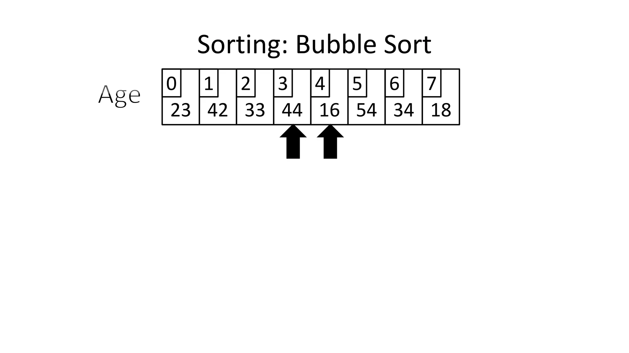
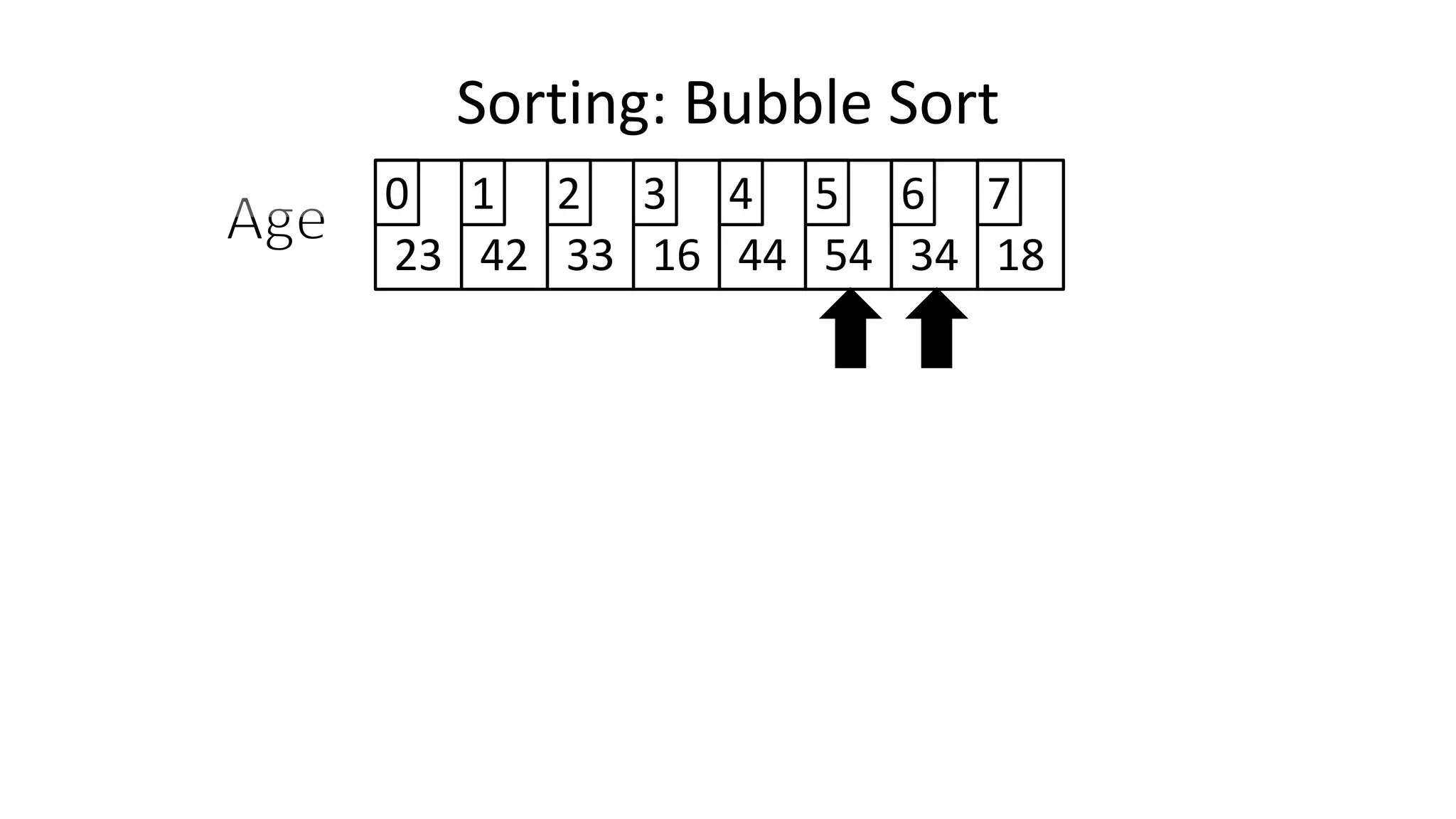
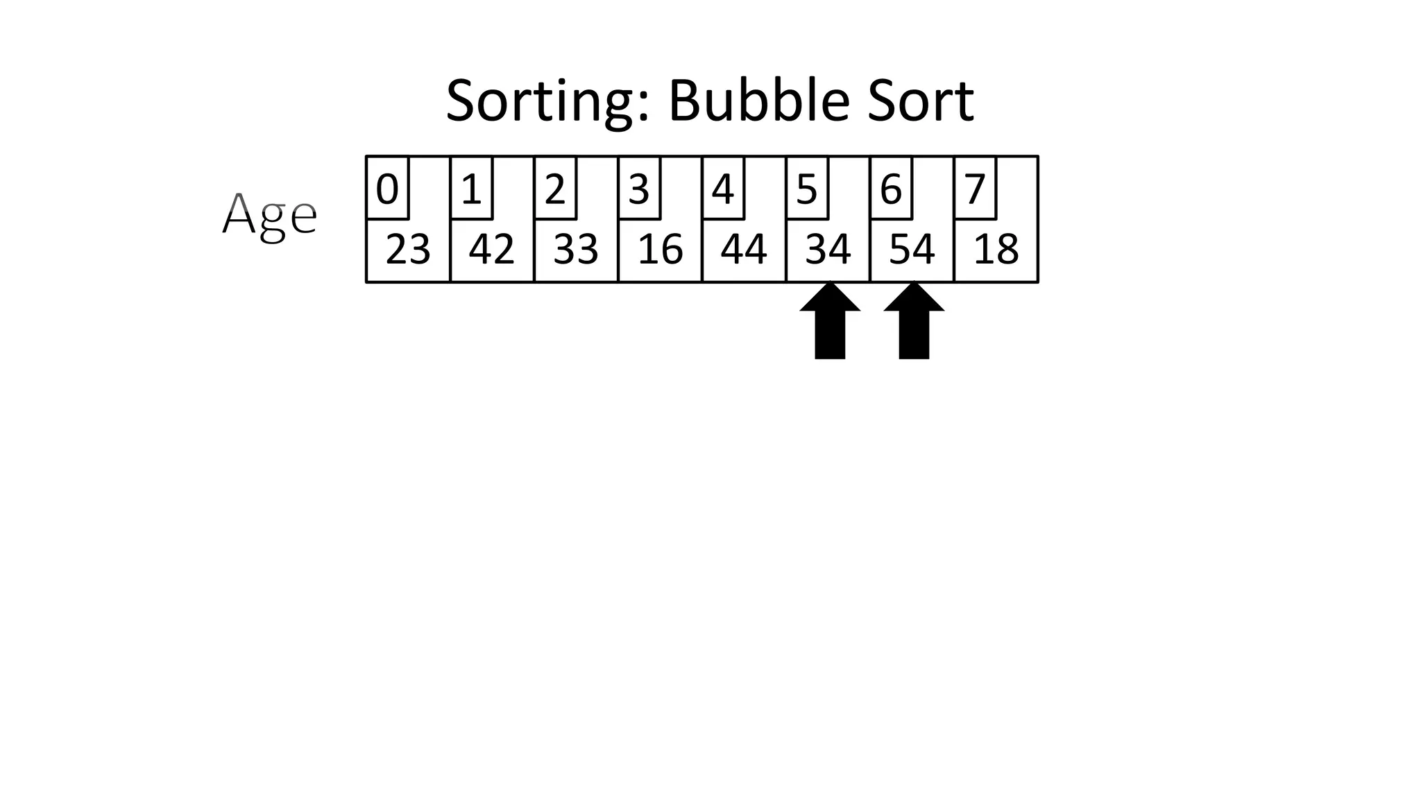
![• To get from one end of the array to another:
FOR Index IN 0 TO N-2
DO IF (Age[Index+1] < Age[Index])
THEN Temp_Value <- Age[Index+1];
Age[Index+1] <- Age[Index];
Age[Index] <- Temp_Value;
ENDIF;
ENDFOR;
Sorting: Bubble Sort](https://image.slidesharecdn.com/completecourse-150726101701-lva1-app6892/75/A-complete-course-in-Program-Design-using-Pseudocode-484-2048.jpg)


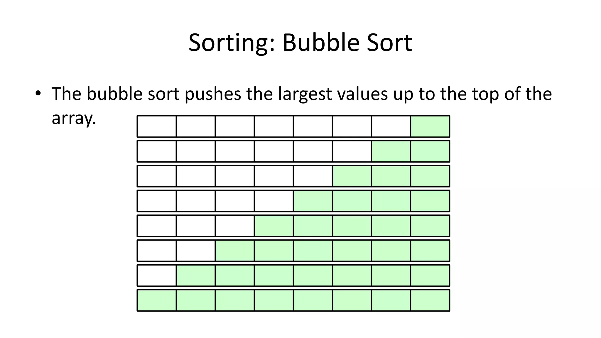
![• So we need two loops:
FOR Outer-Index IN 0 TO N-1
DO FOR Index IN 0 TO N-2
DO IF (Age[Index+1] < Age[Index])
THEN Temp_Value <- Age[Index+1];
Age[Index+1] <- Age[Index];
Age[Index] <- Temp_Value;
ENDIF;
ENDFOR;
ENDFOR;
Sorting: Bubble Sort](https://image.slidesharecdn.com/completecourse-150726101701-lva1-app6892/75/A-complete-course-in-Program-Design-using-Pseudocode-588-2048.jpg)
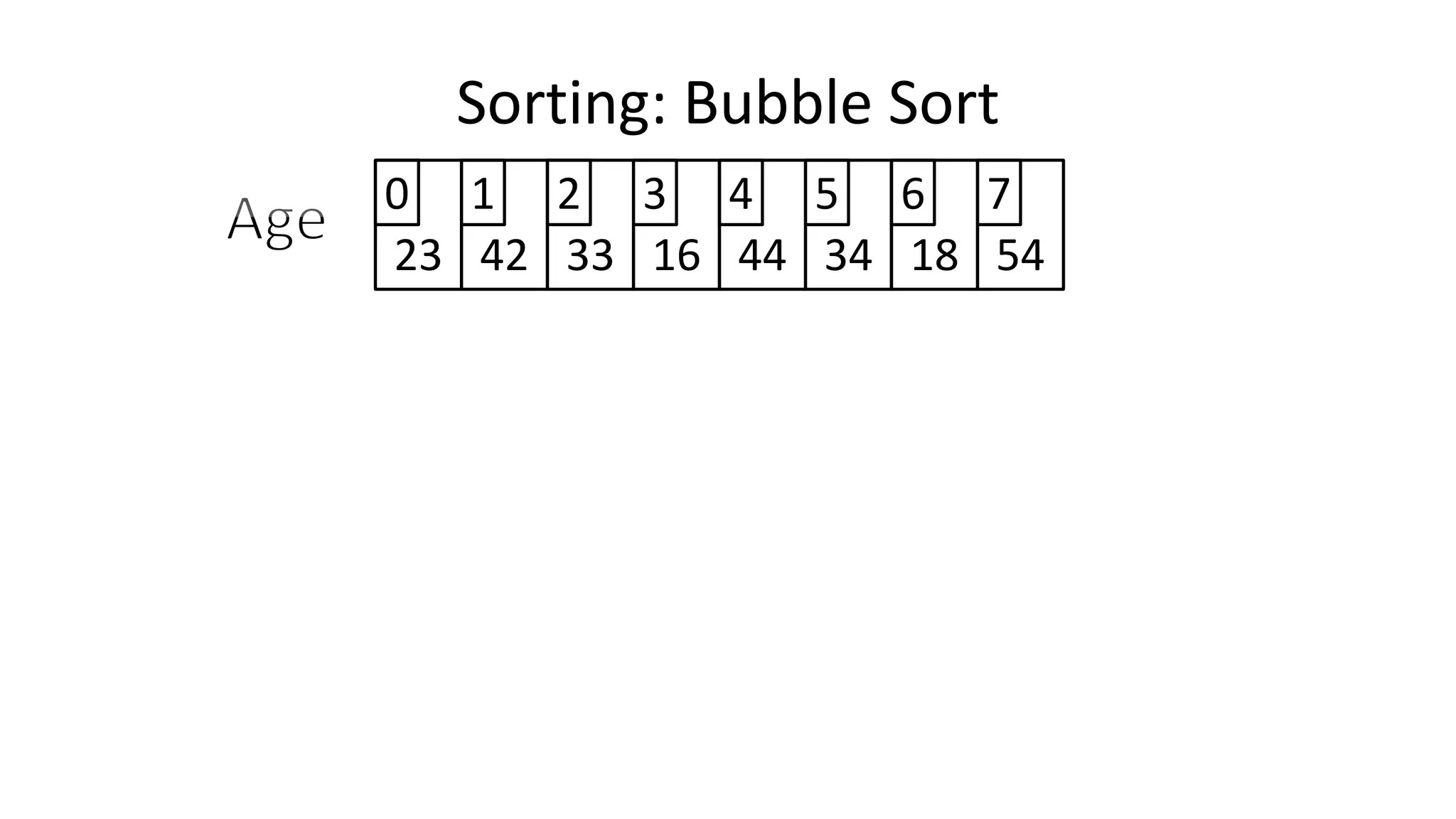
![PROGRAM BubbleSort:
Integer Age[8] <- {44,23,42,33,16,54,34,18};
FOR Outer-Index IN 0 TO N-1
DO FOR Index IN 0 TO N-2
DO IF (Age[Index+1] < Age[Index])
THEN Temp_Value <- Age[Index+1];
Age[Index+1] <- Age[Index];
Age[Index] <- Temp_Value;
ENDIF;
ENDFOR;
ENDFOR;
END.
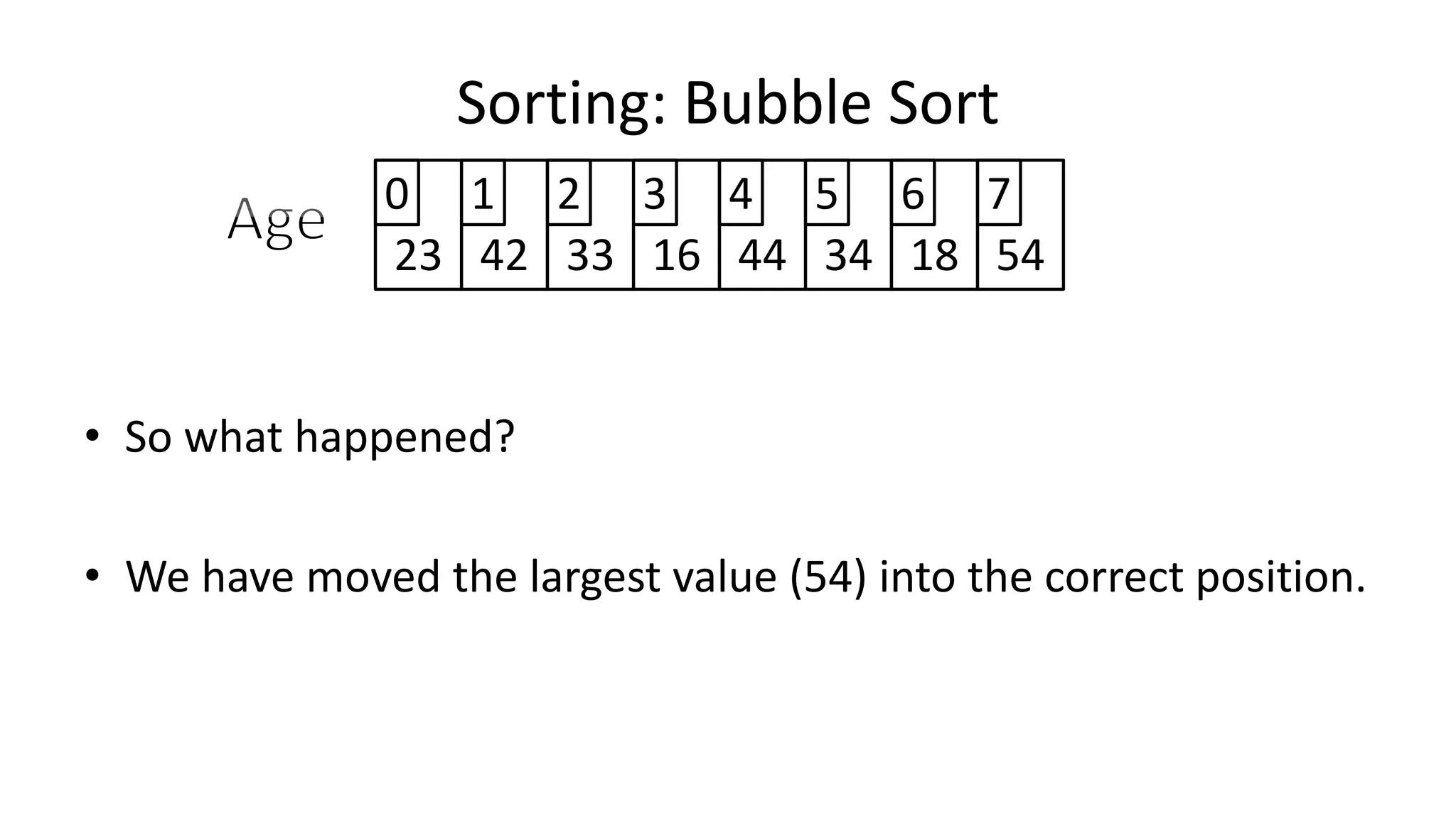
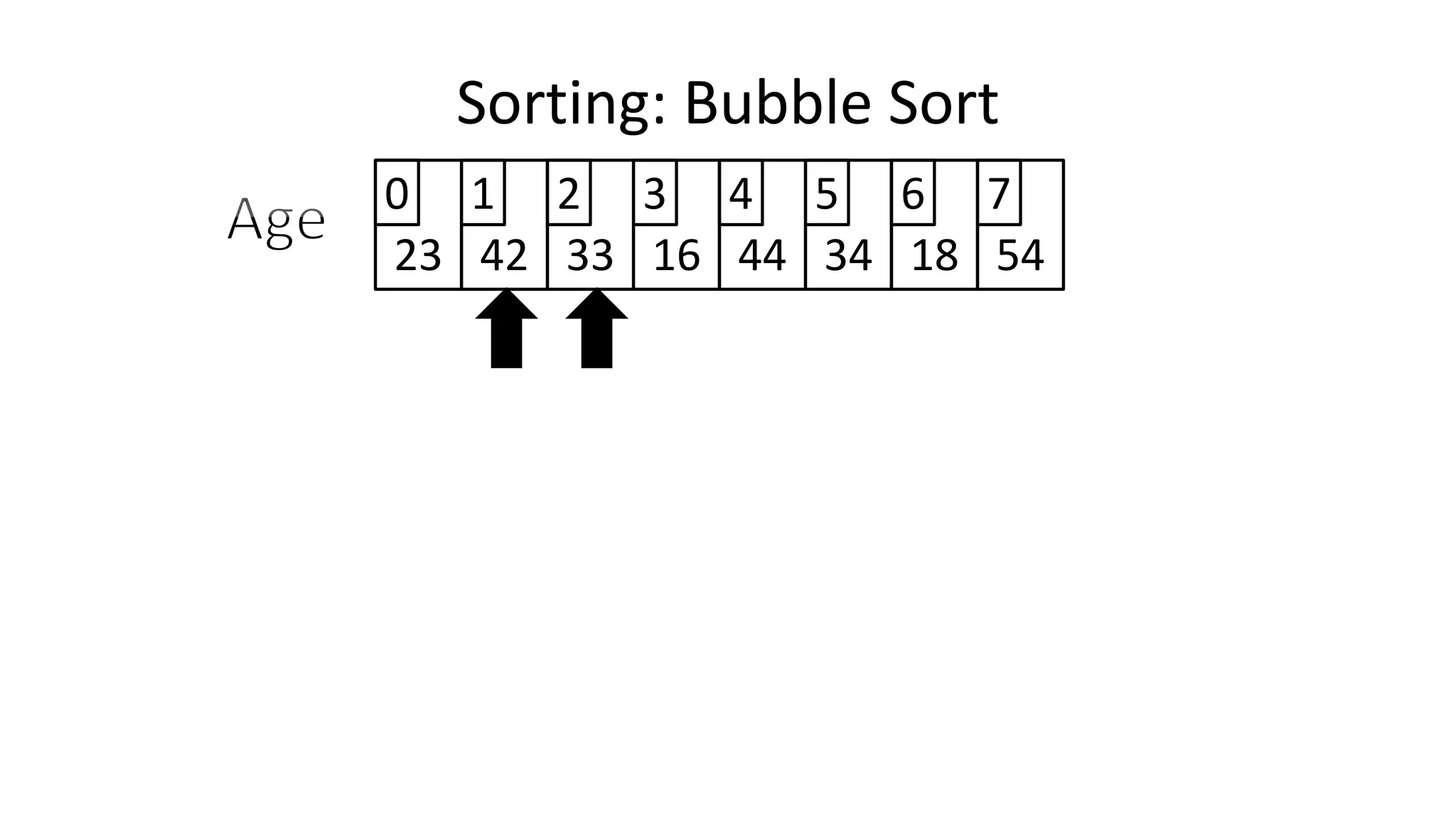
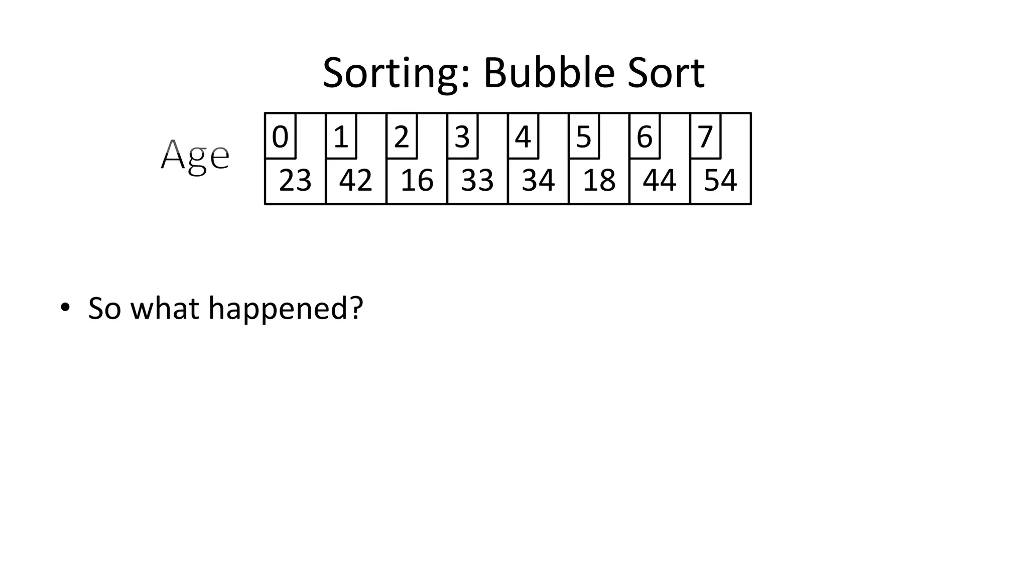
Sorting: Bubble Sort](https://image.slidesharecdn.com/completecourse-150726101701-lva1-app6892/75/A-complete-course-in-Program-Design-using-Pseudocode-589-2048.jpg)


![PROGRAM BubbleSort:
Integer Age[8] <- {44,23,42,33,16,54,34,18};
FOR Outer-Index IN 0 TO N-1
DO FOR Index IN 0 TO N-2
DO IF (Age[Index+1] < Age[Index])
THEN Temp_Value <- Age[Index+1];
Age[Index+1] <- Age[Index];
Age[Index] <- Temp_Value;
ENDIF;
ENDFOR;
ENDFOR;
END.
Sorting: Bubble Sort](https://image.slidesharecdn.com/completecourse-150726101701-lva1-app6892/75/A-complete-course-in-Program-Design-using-Pseudocode-594-2048.jpg)
![PROGRAM BubbleSort:
Integer Age[8] <- {44,23,42,33,16,54,34,18};
ReducingIndex <- N-2;
FOR Outer-Index IN 0 TO N-1
DO FOR Index IN 0 TO ReducingIndex
DO IF (Age[Index+1] < Age[Index])
THEN Temp_Value <- Age[Index+1];
Age[Index+1] <- Age[Index];
Age[Index] <- Temp_Value;
ENDIF;
ENDFOR;
ReducingIndex <- ReducingIndex – 1;
ENDFOR;
END.
Sorting: Bubble Sort](https://image.slidesharecdn.com/completecourse-150726101701-lva1-app6892/75/A-complete-course-in-Program-Design-using-Pseudocode-606-2048.jpg)
![PROGRAM BubbleSort:
Integer Age[8] <- {44,23,42,33,16,54,34,18};
ReducingIndex <- N-2;
FOR Outer-Index IN 0 TO N-1
DO FOR Index IN 0 TO ReducingIndex
DO IF (Age[Index+1] < Age[Index])
THEN Temp_Value <- Age[Index+1];
Age[Index+1] <- Age[Index];
Age[Index] <- Temp_Value;
ENDIF;
ENDFOR;
ReducingIndex <- ReducingIndex – 1;
ENDFOR;
END.
Sorting: Bubble Sort](https://image.slidesharecdn.com/completecourse-150726101701-lva1-app6892/75/A-complete-course-in-Program-Design-using-Pseudocode-607-2048.jpg)
![Sorting: Bubble SortPROGRAM BubbleSort:
Integer Age[8] <- {44,23,42,33,16,54,34,18};
ReducingIndex <- N-2;
DidSwap <- FALSE;
FOR Outer-Index IN 0 TO N-1
DO FOR Index IN 0 TO ReducingIndex
DO IF (Age[Index+1] < Age[Index])
THEN Temp_Value <- Age[Index+1];
Age[Index+1] <- Age[Index];
Age[Index] <- Temp_Value;
DidSwap <- TRUE;
ENDIF;
ENDFOR;
ReducingIndex <- ReducingIndex – 1;
IF (DidSwap = FALSE)
THEN EXIT;
ENDIF;
ENDFOR;
END.](https://image.slidesharecdn.com/completecourse-150726101701-lva1-app6892/75/A-complete-course-in-Program-Design-using-Pseudocode-609-2048.jpg)
![PROGRAM BubbleSort:
Integer Age[8] <- {44,23,42,33,16,54,34,18};
ReducingIndex <- N-2;
DidSwap <- FALSE;
FOR Outer-Index IN 0 TO N-1
DO FOR Index IN 0 TO ReducingIndex
DO IF (Age[Index+1] < Age[Index])
THEN Temp_Value <- Age[Index+1];
Age[Index+1] <- Age[Index];
Age[Index] <- Temp_Value;
DidSwap <- TRUE;
ENDIF;
ENDFOR;
ReducingIndex <- ReducingIndex – 1;
IF (DidSwap = FALSE)
THEN EXIT;
ENDIF;
ENDFOR;
END.
Sorting: Bubble Sort](https://image.slidesharecdn.com/completecourse-150726101701-lva1-app6892/75/A-complete-course-in-Program-Design-using-Pseudocode-610-2048.jpg)
![MODULE SWAP[A,B]:
Integer Temp_Value
Temp_Value <- B;
B <- A;
A <- Temp_Value;
RETURN A, B;
END.
Sorting: Bubble Sort](https://image.slidesharecdn.com/completecourse-150726101701-lva1-app6892/75/A-complete-course-in-Program-Design-using-Pseudocode-612-2048.jpg)
![PROGRAM BubbleSort:
Integer Age[8] <- {44,23,42,33,16,54,34,18};
ReducingIndex <- N-2;
DidSwap <- FALSE;
FOR Outer-Index IN 0 TO N-1
DO FOR Index IN 0 TO ReducingIndex
DO IF (Age[Index+1] < Age[Index])
THEN Temp_Value <- Age[Index+1];
Age[Index+1] <- Age[Index];
Age[Index] <- Temp_Value;
DidSwap <- TRUE;
ENDIF;
ENDFOR;
ReducingIndex <- ReducingIndex – 1;
IF (DidSwap = FALSE)
THEN EXIT;
ENDIF;
ENDFOR;
END.
Sorting: Bubble Sort](https://image.slidesharecdn.com/completecourse-150726101701-lva1-app6892/75/A-complete-course-in-Program-Design-using-Pseudocode-613-2048.jpg)
![PROGRAM BubbleSort:
Integer Age[8] <- {44,23,42,33,16,54,34,18};
ReducingIndex <- N-2;
DidSwap <- FALSE;
FOR Outer-Index IN 0 TO N-1
DO FOR Index IN 0 TO ReducingIndex
DO IF (Age[Index+1] < Age[Index])
THEN Temp_Value <- Age[Index+1];
Age[Index+1] <- Age[Index];
Age[Index] <- Temp_Value;
DidSwap <- TRUE;
ENDIF;
ENDFOR;
ReducingIndex <- ReducingIndex – 1;
IF (DidSwap = FALSE)
THEN EXIT;
ENDIF;
ENDFOR;
END.
Sorting: Bubble Sort](https://image.slidesharecdn.com/completecourse-150726101701-lva1-app6892/75/A-complete-course-in-Program-Design-using-Pseudocode-614-2048.jpg)
![PROGRAM BubbleSort:
Integer Age[8] <- {44,23,42,33,16,54,34,18};
ReducingIndex <- N-2;
DidSwap <- FALSE;
FOR Outer-Index IN 0 TO N-1
DO FOR Index IN 0 TO ReducingIndex
DO IF (Age[Index+1] < Age[Index])
THEN SWAP(Age[Index], Age[Index+1];
DidSwap <- TRUE;
ENDIF;
ENDFOR;
ReducingIndex <- ReducingIndex – 1;
IF (DidSwap = FALSE)
THEN EXIT;
ENDIF;
ENDFOR;
END.
Sorting: Bubble Sort](https://image.slidesharecdn.com/completecourse-150726101701-lva1-app6892/75/A-complete-course-in-Program-Design-using-Pseudocode-615-2048.jpg)


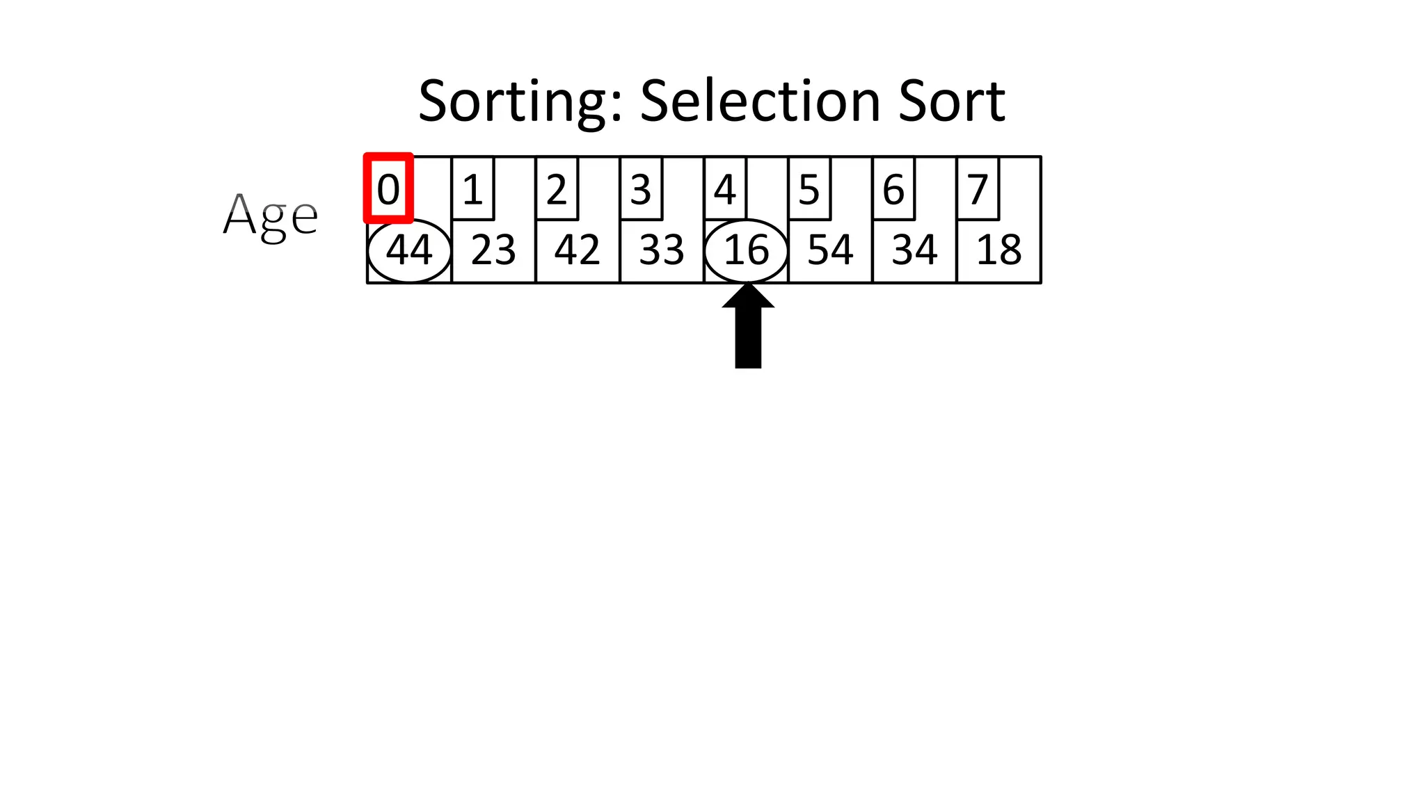


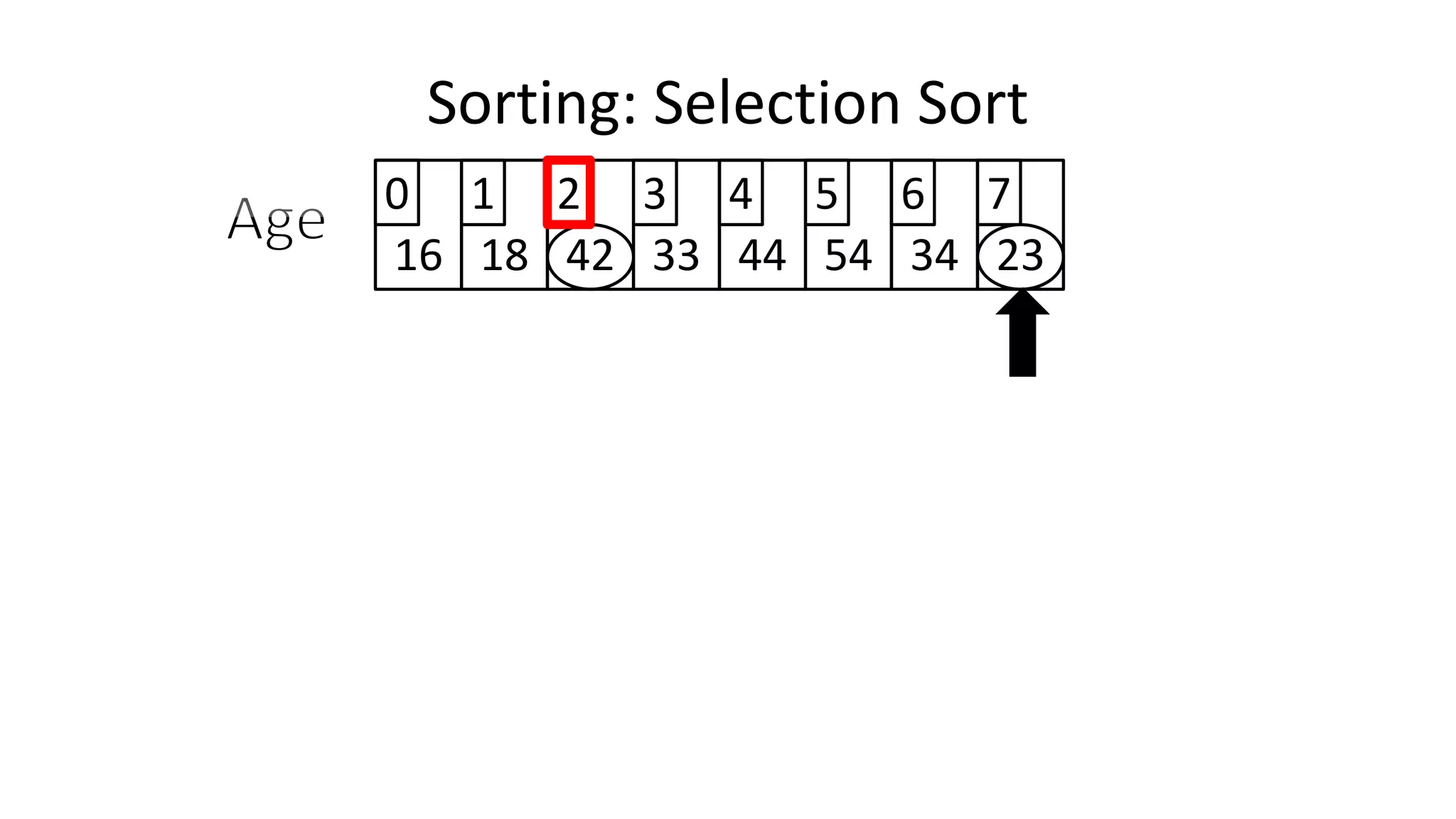

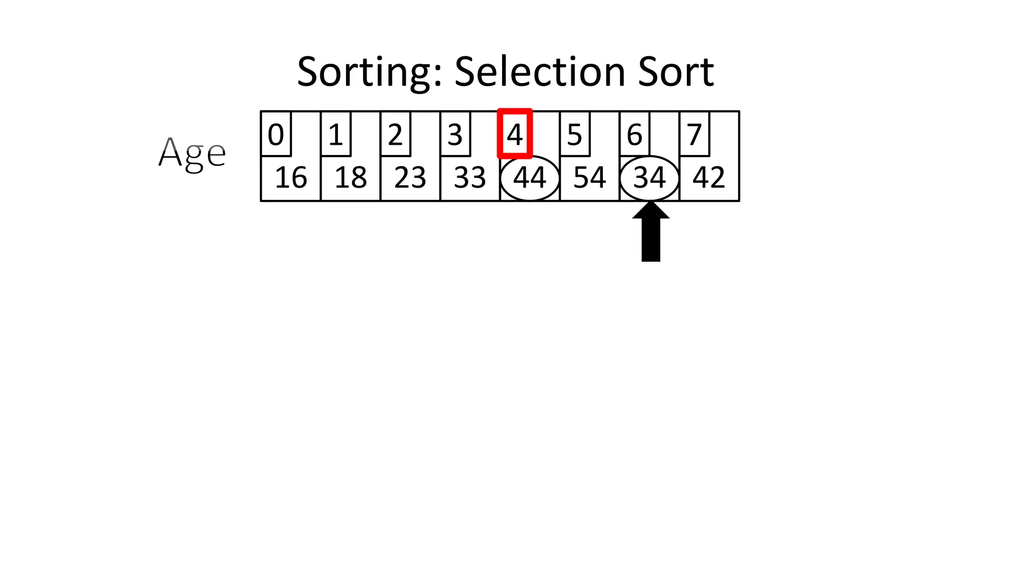


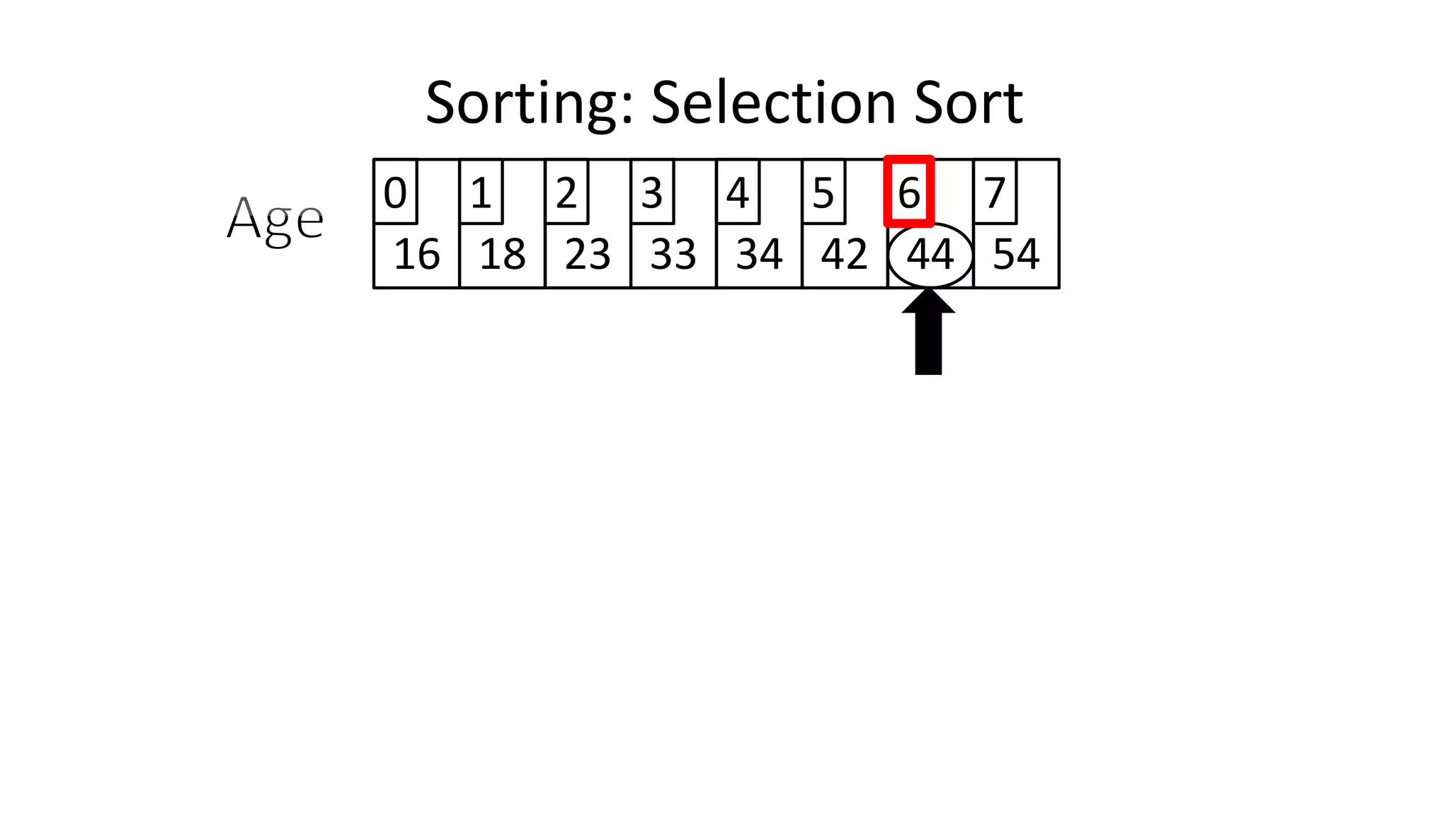
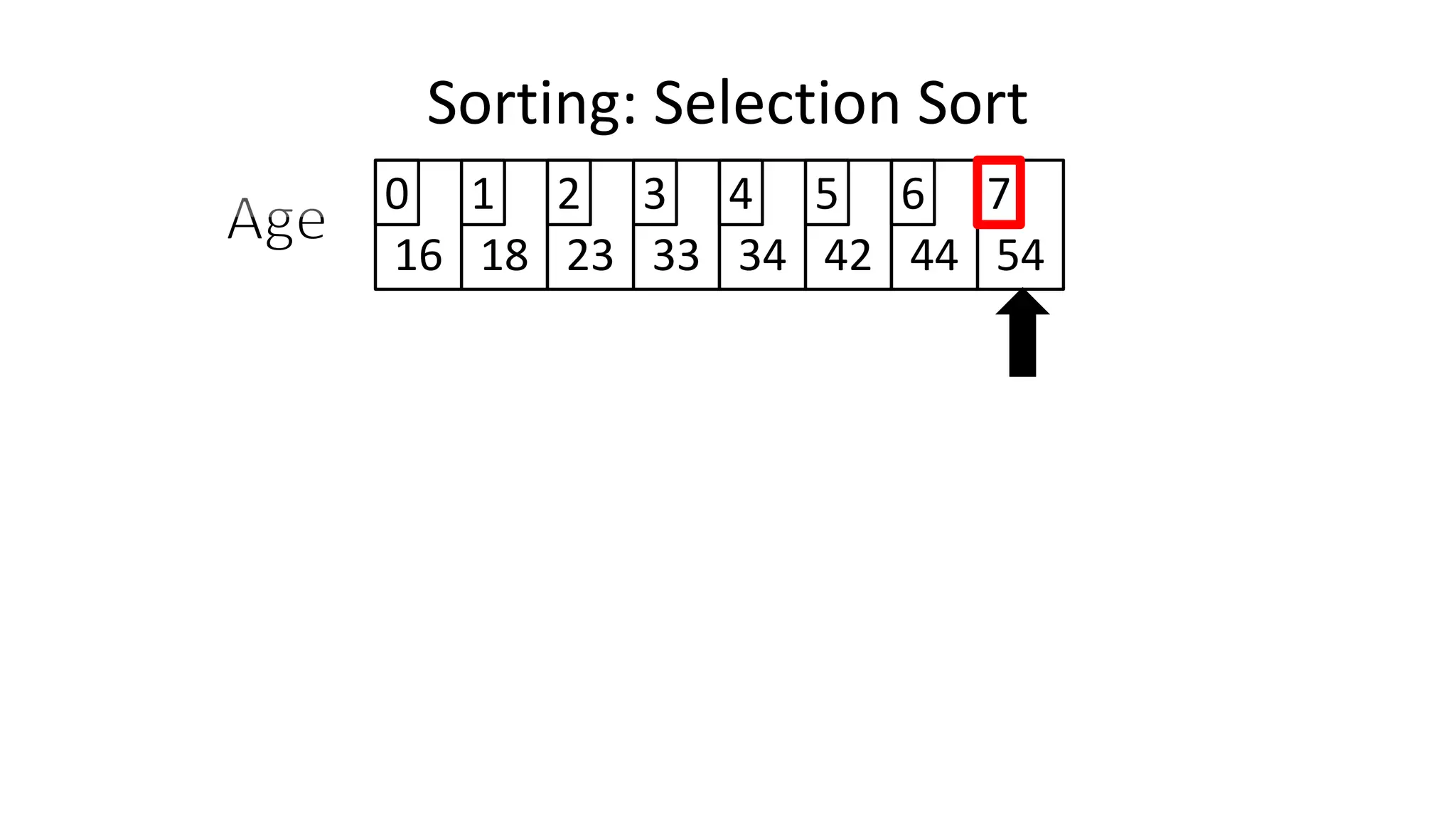
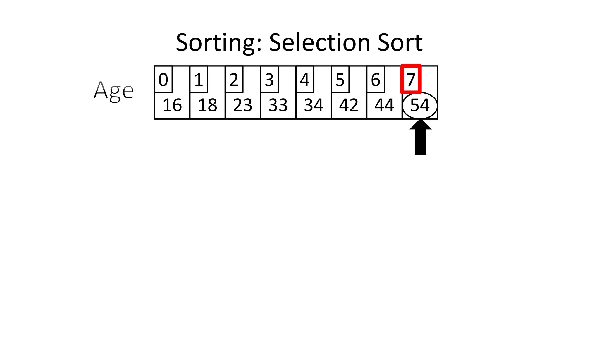
![Sorting: Selection Sort
• So we know we only have to swap if the value is not already in
the correct location.
• This will look a little something like this:
IF (MinValueLocation != CurrentLocation)
THEN Swap(Age[CurrentLocation], Age[MinValueLocation];
ENDIF;](https://image.slidesharecdn.com/completecourse-150726101701-lva1-app6892/75/A-complete-course-in-Program-Design-using-Pseudocode-644-2048.jpg)
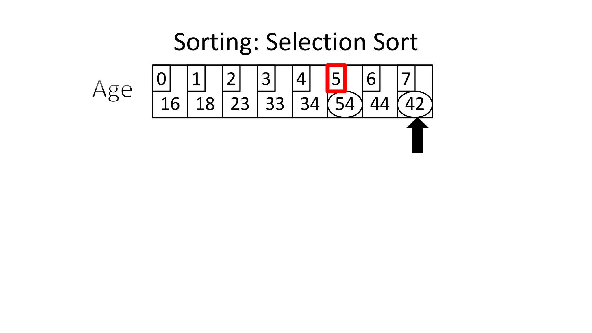
![• We will find the minimum value in the list using something like
the following:
MinValueLocation <- 0;
FOR Index IN IncreasingCount TO N-1
DO IF (Age[Index] < Age[MinValueLocation])
THEN MinValueLocation <- Index;
ENDIF;
ENDFOR;
Sorting: Selection Sort](https://image.slidesharecdn.com/completecourse-150726101701-lva1-app6892/75/A-complete-course-in-Program-Design-using-Pseudocode-645-2048.jpg)

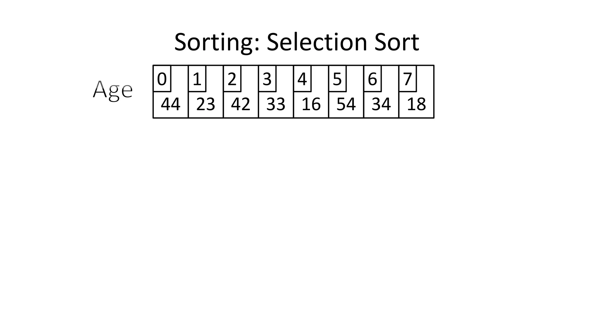
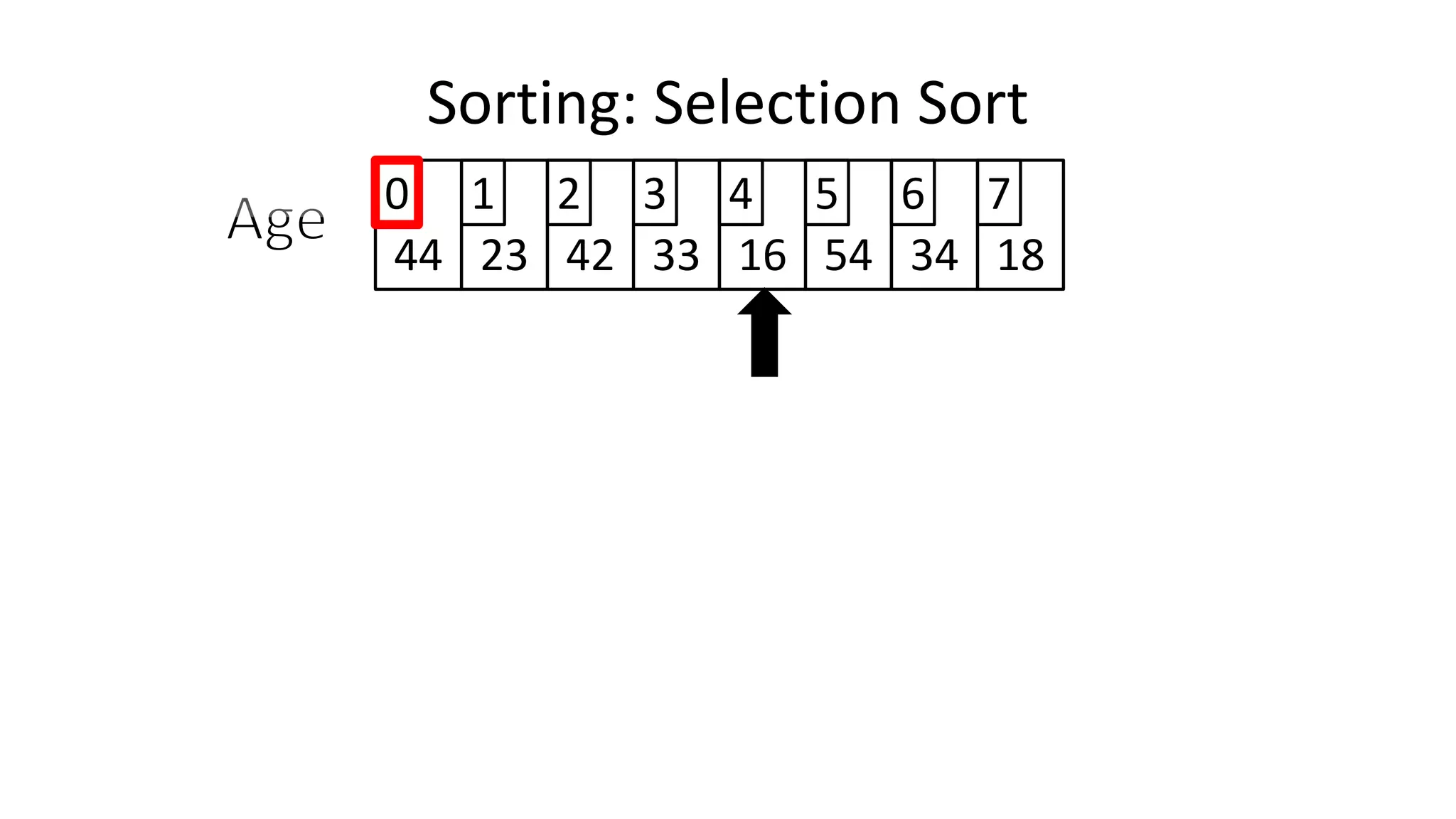
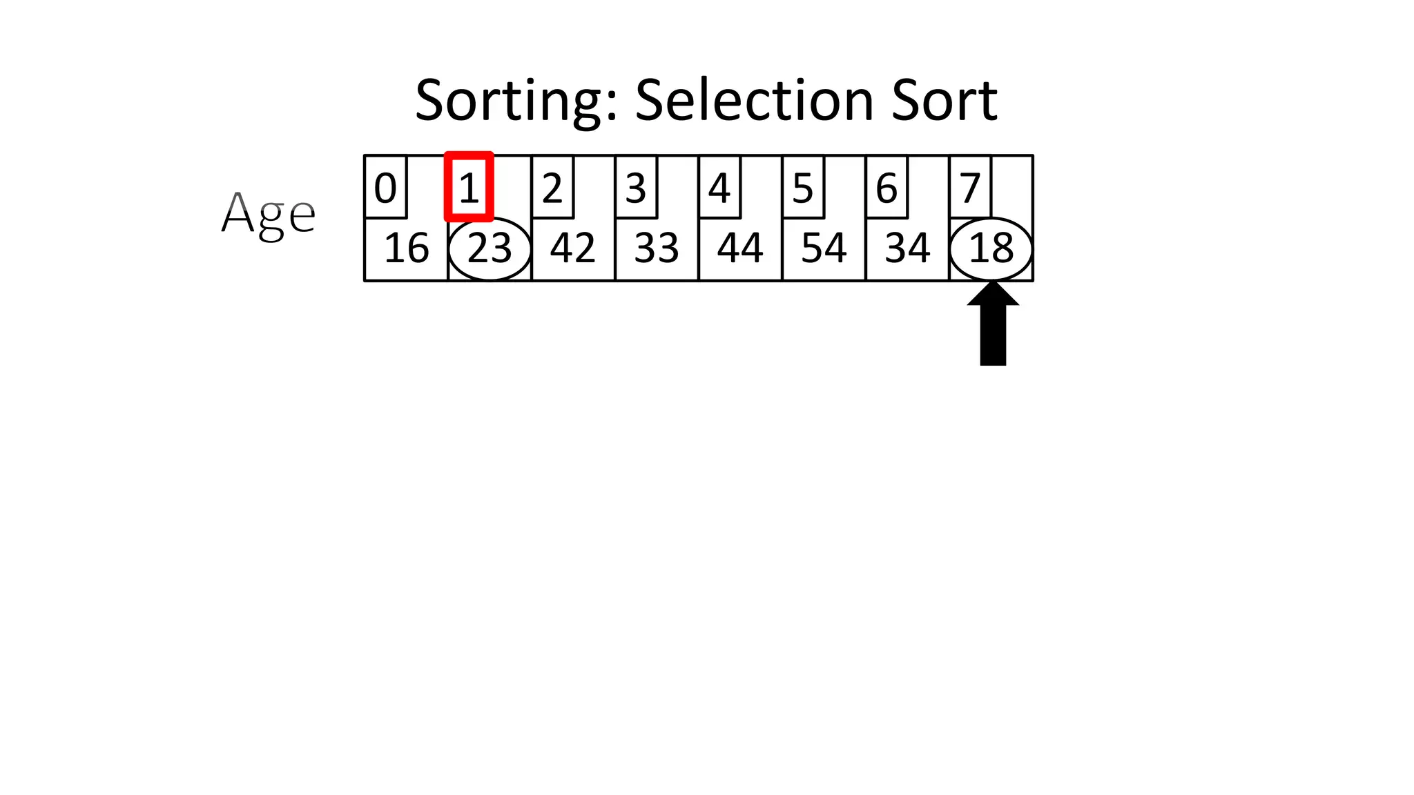
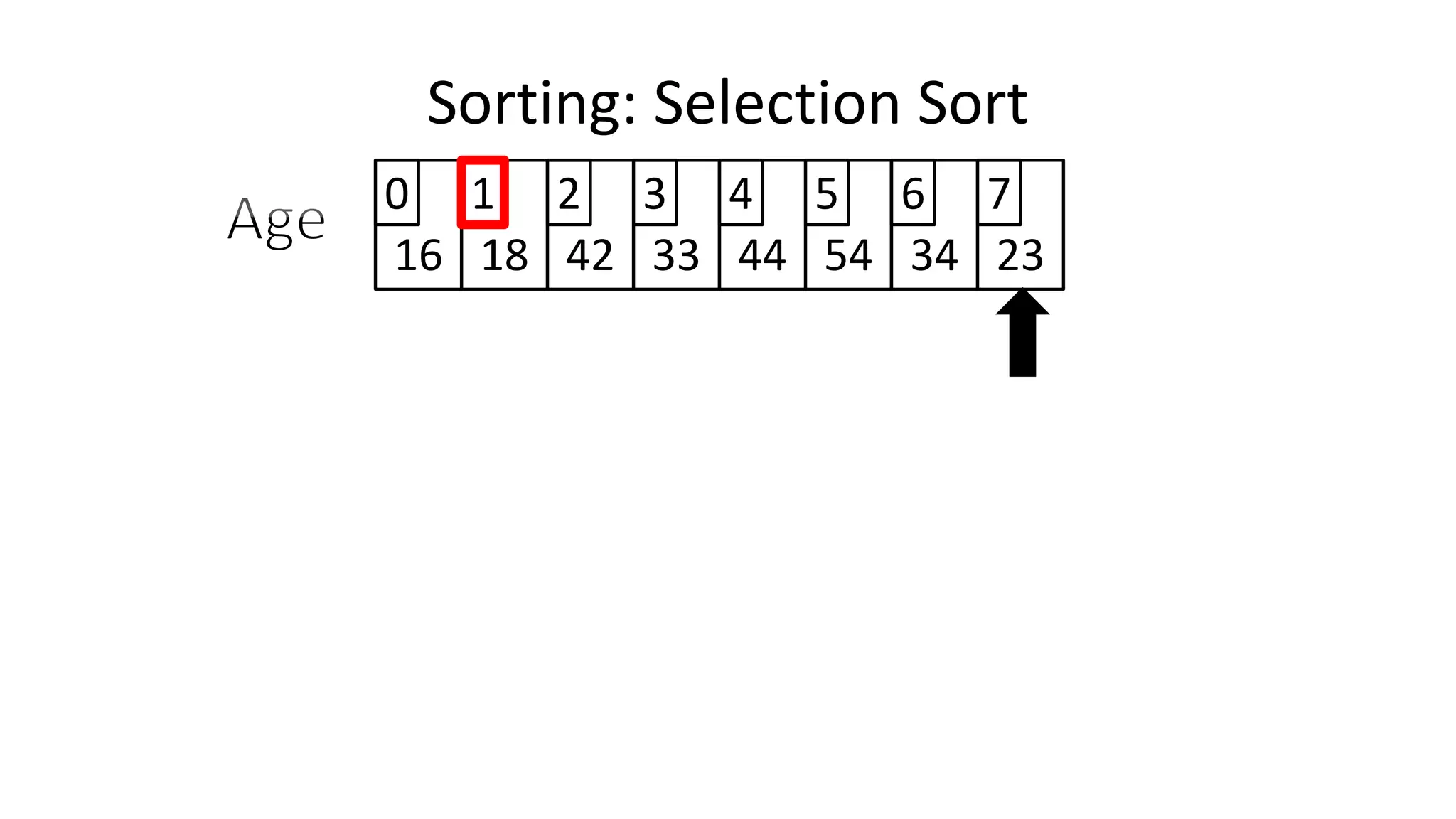
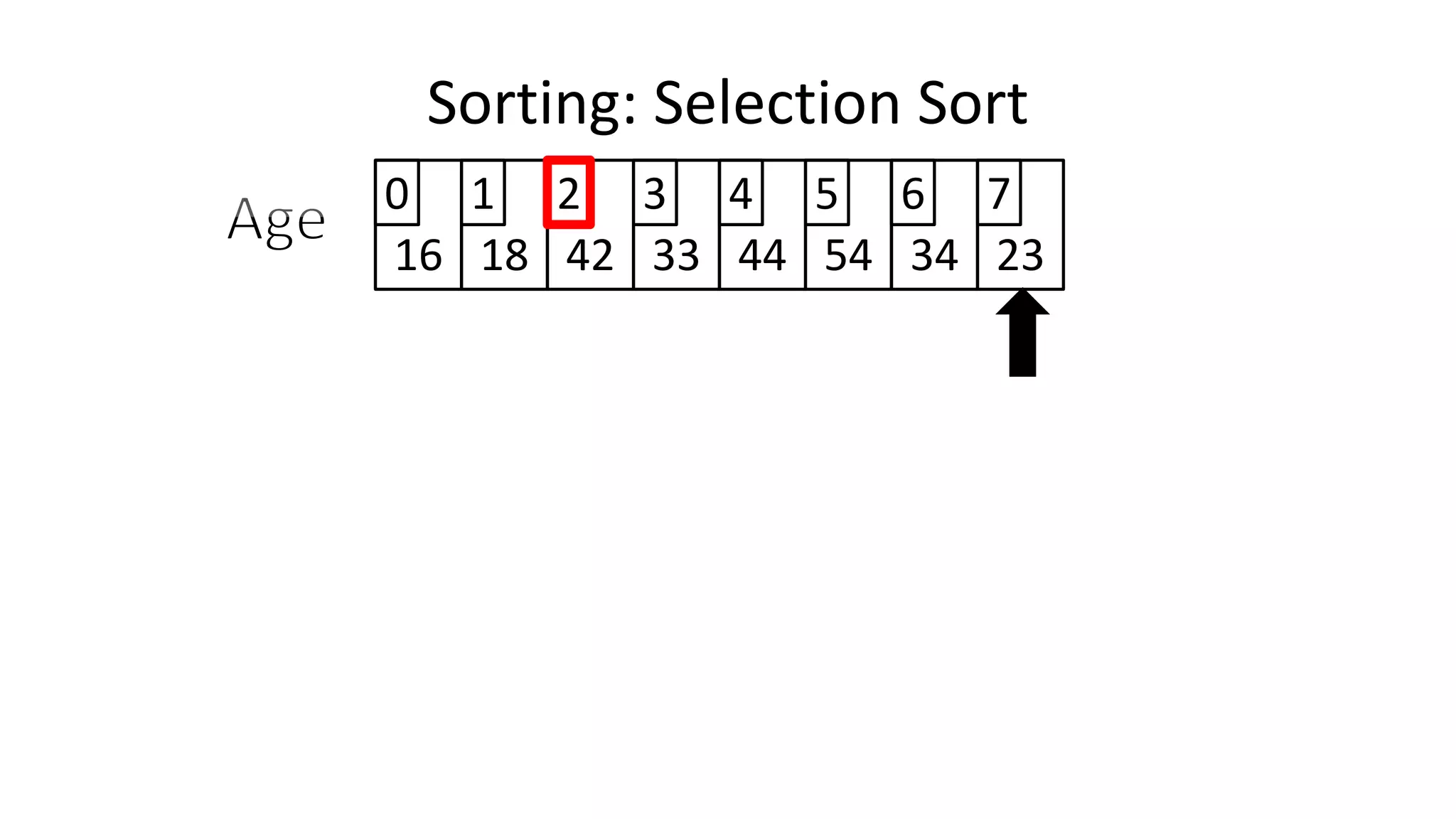
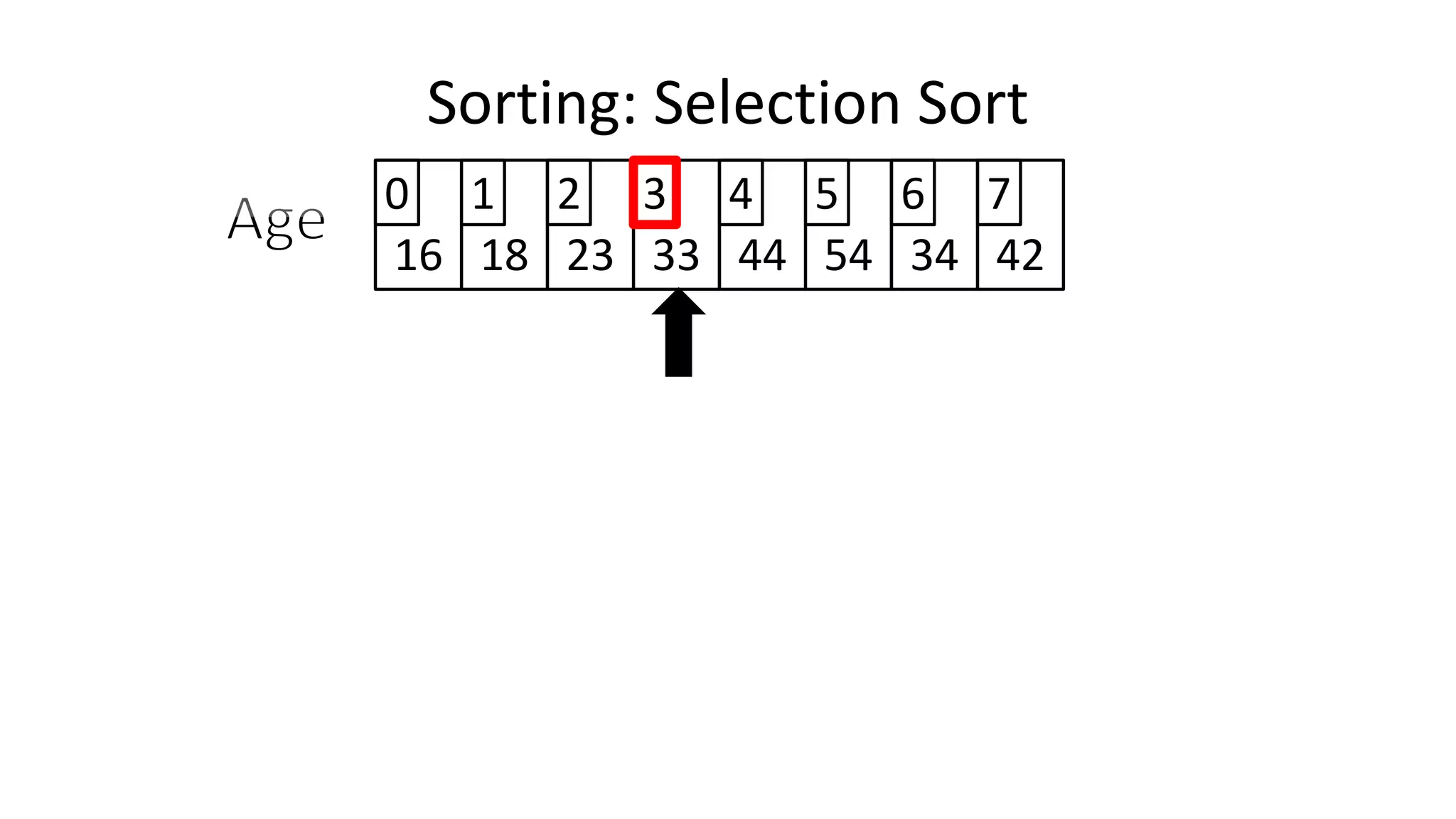
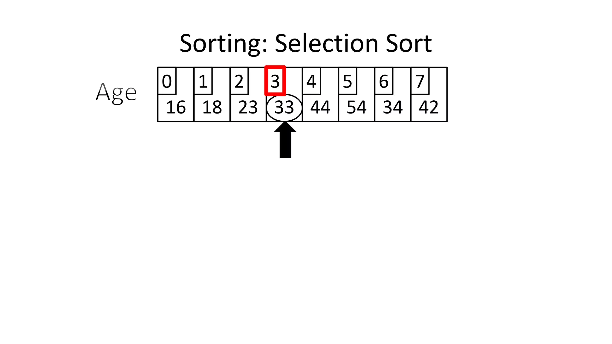
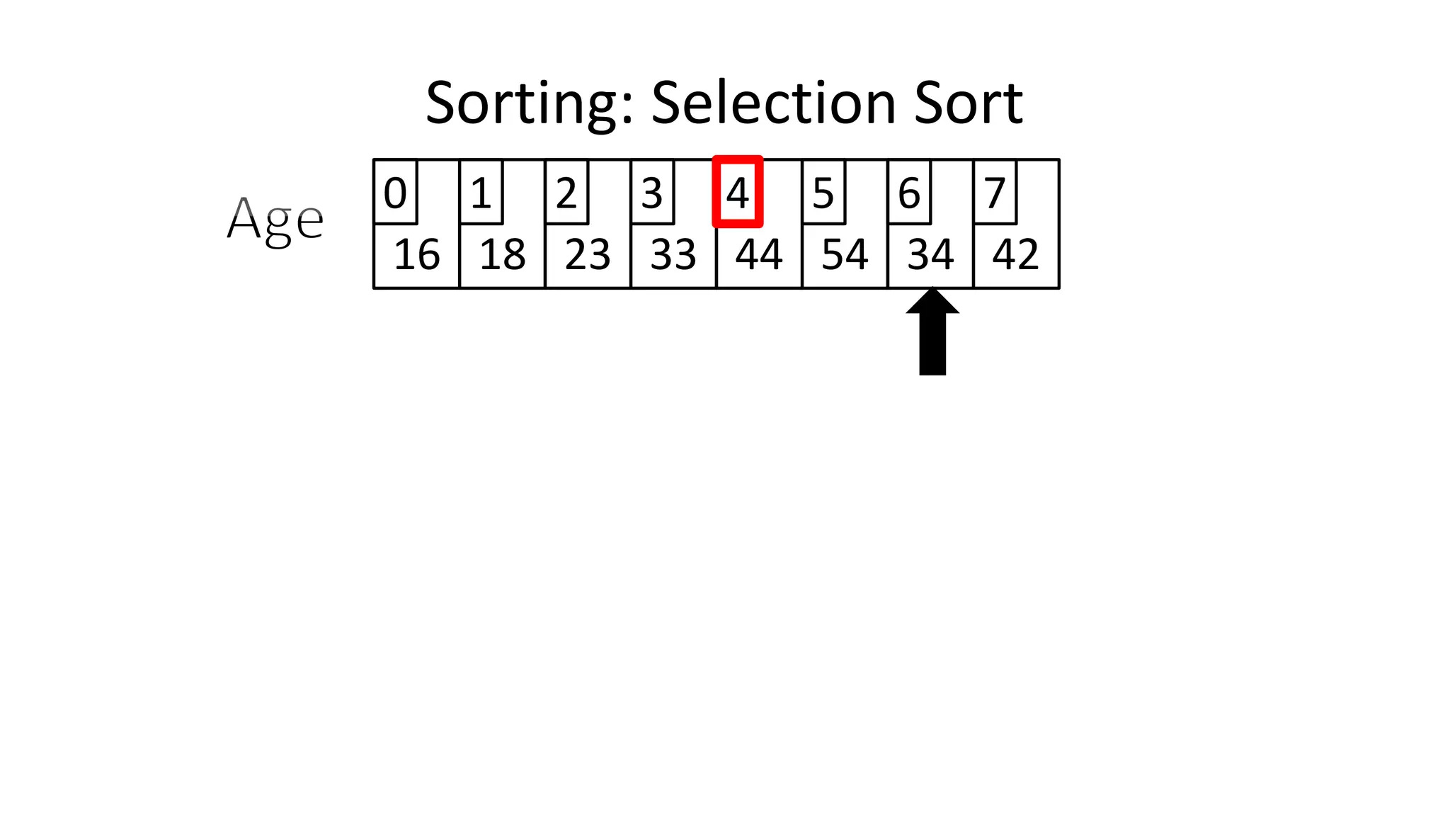
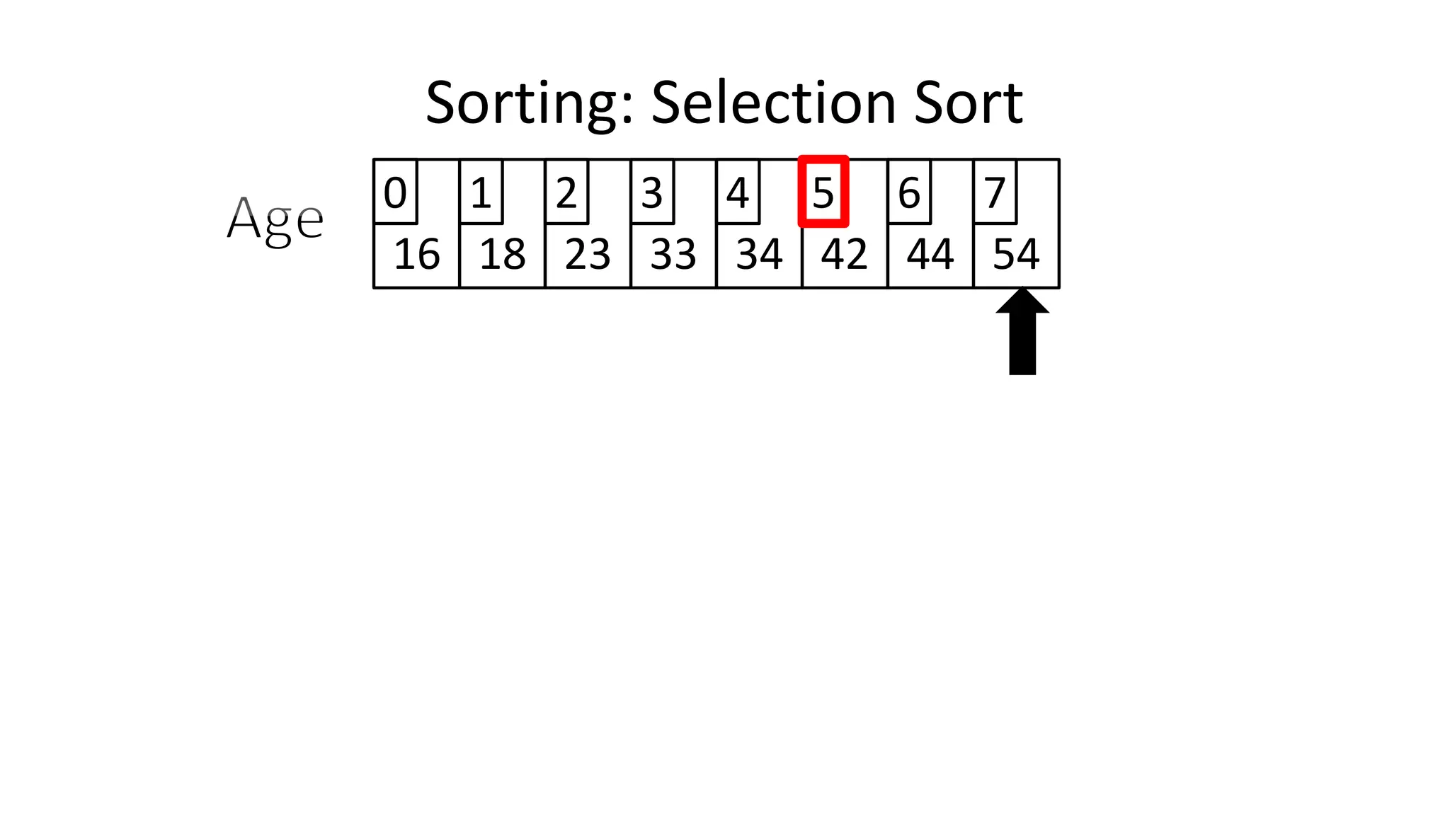
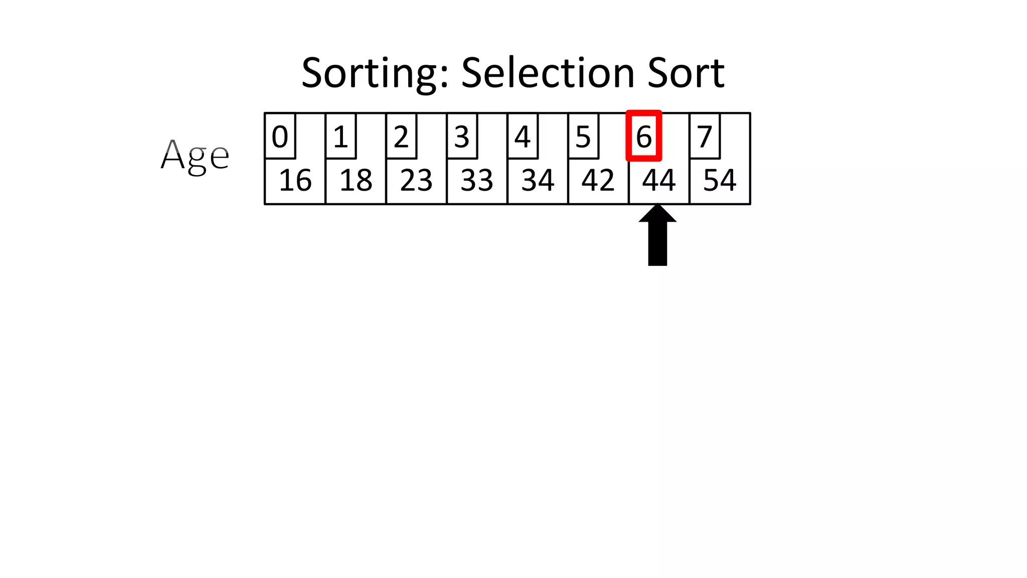
![PROGRAM SelectionSort:
Integer Age[8] <- {44,23,42,33,16,54,34,18};
FOR Outer-Index IN 0 TO N-1
MinValueLocation <- Outer-Index;
FOR Index IN Outer-Index+1 TO N-1
DO IF (Age[Index] < Age[MinValueLocation])
THEN MinValueLocation <- Index;
ENDIF;
ENDFOR;
IF (MinValueLocation != Outer-Index)
THEN Swap(Age[Outer-Index], Age[MinValueLocation]);
ENDIF;
ENDFOR;
END.
Sorting: Selection Sort](https://image.slidesharecdn.com/completecourse-150726101701-lva1-app6892/75/A-complete-course-in-Program-Design-using-Pseudocode-647-2048.jpg)


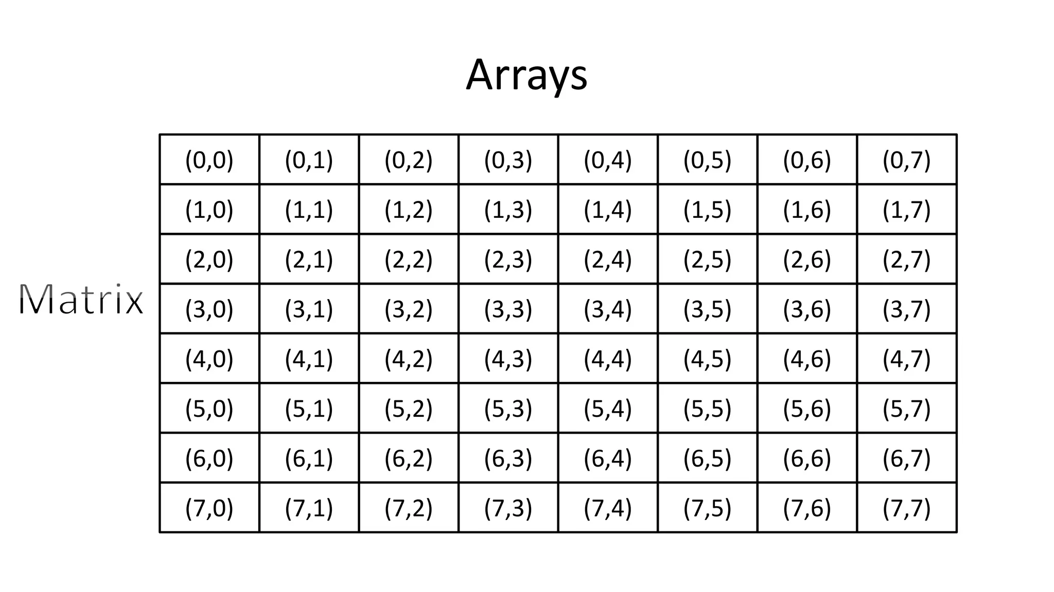
![Arrays
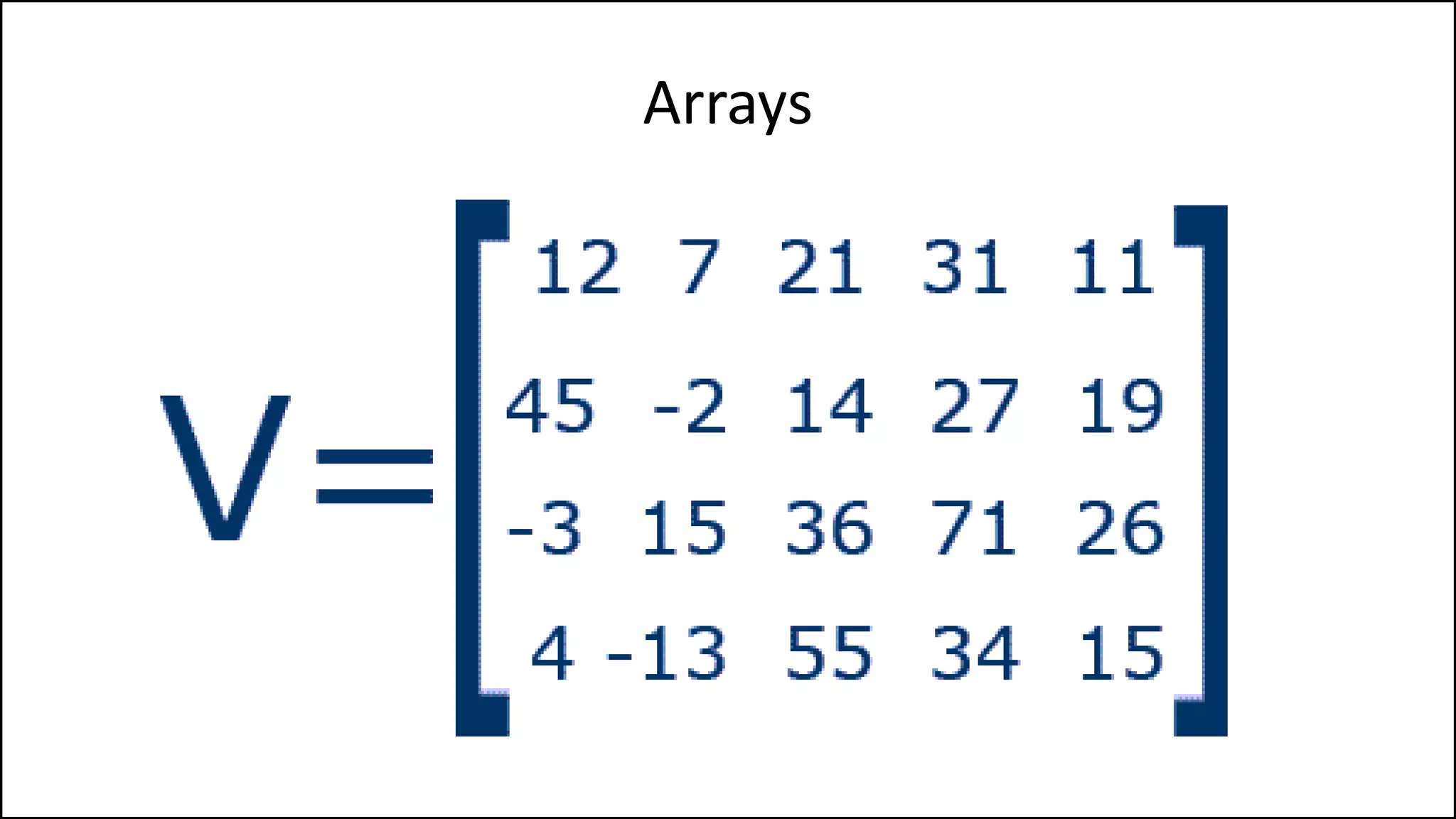
• We declare a multi-dimensional array as follows:
• Integer Age[8][8];](https://image.slidesharecdn.com/completecourse-150726101701-lva1-app6892/75/A-complete-course-in-Program-Design-using-Pseudocode-659-2048.jpg)
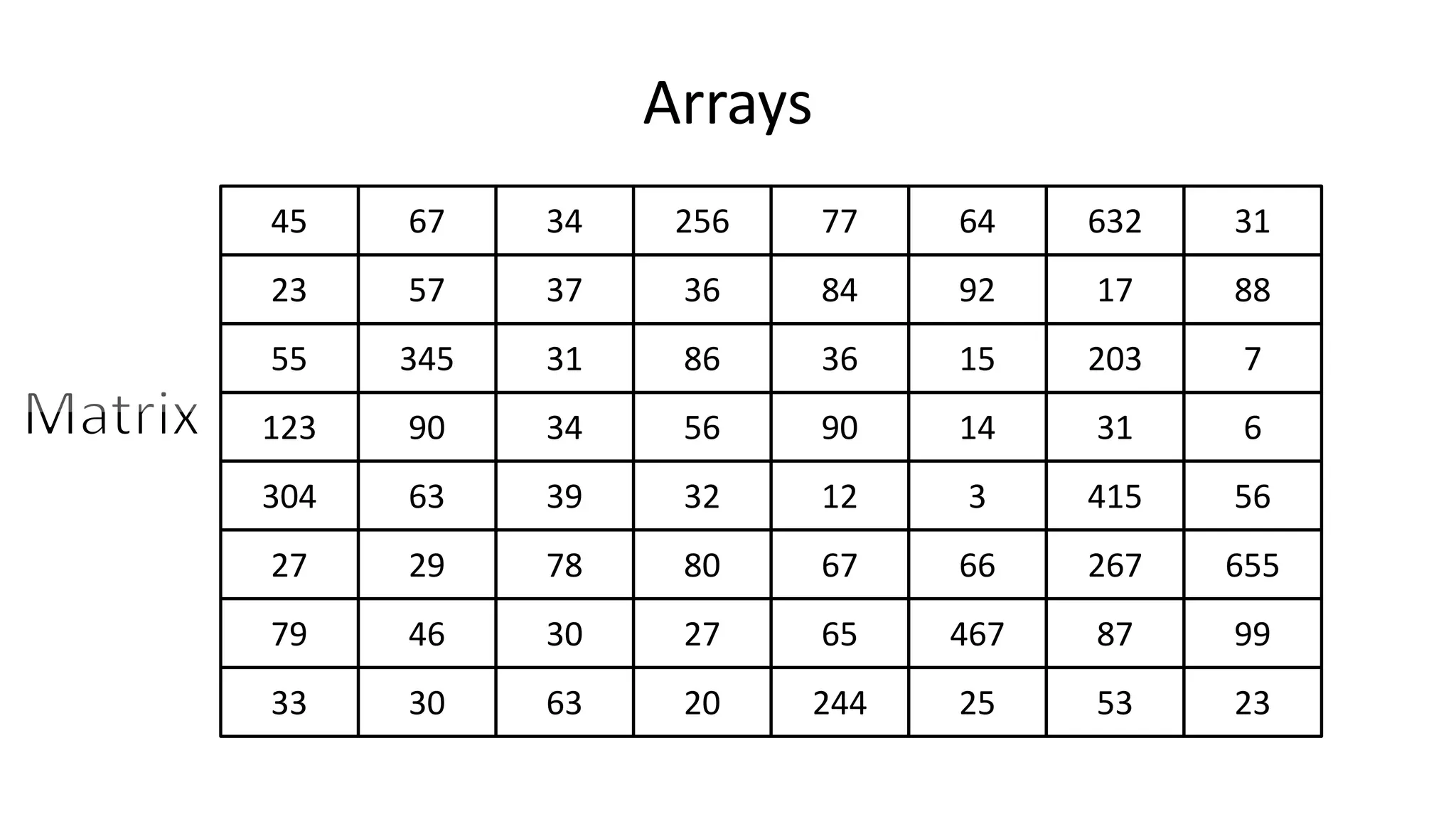
![Arrays
• So if I do:
• PRINT Matrix[0][0];
• We will get:
• 45](https://image.slidesharecdn.com/completecourse-150726101701-lva1-app6892/75/A-complete-course-in-Program-Design-using-Pseudocode-664-2048.jpg)
![Arrays
• So if I do:
• PRINT Matrix[2][0];
• We will get:
• 55](https://image.slidesharecdn.com/completecourse-150726101701-lva1-app6892/75/A-complete-course-in-Program-Design-using-Pseudocode-665-2048.jpg)
![Arrays
• So if I do:
• PRINT Matrix[0][2];
• We will get:
• 34](https://image.slidesharecdn.com/completecourse-150726101701-lva1-app6892/75/A-complete-course-in-Program-Design-using-Pseudocode-666-2048.jpg)
![Arrays
• So if I do:
• PRINT Matrix[7][7];
• We will get:
• 23](https://image.slidesharecdn.com/completecourse-150726101701-lva1-app6892/75/A-complete-course-in-Program-Design-using-Pseudocode-667-2048.jpg)
![Arrays
• So if I do:
• Matrix[5][4] <- 43;
• We will get:
• 67 changed to 43](https://image.slidesharecdn.com/completecourse-150726101701-lva1-app6892/75/A-complete-course-in-Program-Design-using-Pseudocode-668-2048.jpg)
![Arrays
PROGRAM Add1ToMartix:
FOR N IN 0 TO 7
FOR M IN 0 TO 7
DO Matrix[N][M] <- Matrix [N][M] + 1;
ENDFOR;
ENDFOR;
END.](https://image.slidesharecdn.com/completecourse-150726101701-lva1-app6892/75/A-complete-course-in-Program-Design-using-Pseudocode-670-2048.jpg)
![Arrays
Or:
PROGRAM Add1ToMartix:
FOR ROW IN 0 TO 7
FOR COLUMN IN 0 TO 7
DO Matrix[ROW][COLUMN] <- Matrix [ROW][COLUMN] + 1;
ENDFOR;
ENDFOR;
END.](https://image.slidesharecdn.com/completecourse-150726101701-lva1-app6892/75/A-complete-course-in-Program-Design-using-Pseudocode-671-2048.jpg)

![Arrays
PROGRAM TotalOfMatrix:
integer Total <- 0;
FOR N IN 0 TO 7
FOR M IN 0 TO 7
DO Total <- Total + Matrix[N][M];
ENDFOR;
ENDFOR;
END.](https://image.slidesharecdn.com/completecourse-150726101701-lva1-app6892/75/A-complete-course-in-Program-Design-using-Pseudocode-673-2048.jpg)
![Arrays
• We can create a 3D array: Array[N][N][N]
• We can create a 4D array: Array[N][N][N][N]
• We can create a 5D array: Array[N][N][N][N][N]
• etc.](https://image.slidesharecdn.com/completecourse-150726101701-lva1-app6892/75/A-complete-course-in-Program-Design-using-Pseudocode-675-2048.jpg)


![Boolean Logic
PROGRAM GetGrade:
Read Result;
IF (A = 5 AND Age[Index] < Age[Index+1])
THEN PRINT “A is 5”;
ENDIF;
END.](https://crownmelresort.com/image.slidesharecdn.com/completecourse-150726101701-lva1-app6892/75/A-complete-course-in-Program-Design-using-Pseudocode-154-2048.jpg)
![Boolean Logic
PROGRAM GetGrade:
Read Result;
IF (A = 5 AND Age[Index] < Age[Index+1])
THEN PRINT “A is 5”;
ENDIF;
END.
• Both A=5 and Age[Index] < Age[Index+1] must be
TRUE to do the THEN part of the statement.](https://crownmelresort.com/image.slidesharecdn.com/completecourse-150726101701-lva1-app6892/75/A-complete-course-in-Program-Design-using-Pseudocode-155-2048.jpg)

![Boolean Logic
PROGRAM GetGrade:
Read Result;
IF (A = 5 OR Age[Index] < Age[Index+1])
THEN PRINT “A is 5”;
ENDIF;
END.](https://crownmelresort.com/image.slidesharecdn.com/completecourse-150726101701-lva1-app6892/75/A-complete-course-in-Program-Design-using-Pseudocode-157-2048.jpg)
![Boolean Logic
PROGRAM GetGrade:
Read Result;
IF (A = 5 OR Age[Index] < Age[Index+1])
THEN PRINT “A is 5”;
ENDIF;
END.
• Either or both of A=5 and Age[Index] <
Age[Index+1] must be TRUE to do the THEN part of the
statement.](https://crownmelresort.com/image.slidesharecdn.com/completecourse-150726101701-lva1-app6892/75/A-complete-course-in-Program-Design-using-Pseudocode-158-2048.jpg)


![Arrays
• We declare an array as follows:
• Integer Age[40];](https://crownmelresort.com/image.slidesharecdn.com/completecourse-150726101701-lva1-app6892/75/A-complete-course-in-Program-Design-using-Pseudocode-325-2048.jpg)
![Arrays
• We declare an array as follows:
• Integer Age[40];
• Which means we declare 40 integer variables, all can be
accessed using the Age name.
……..…](https://crownmelresort.com/image.slidesharecdn.com/completecourse-150726101701-lva1-app6892/75/A-complete-course-in-Program-Design-using-Pseudocode-326-2048.jpg)
![Arrays
• We declare an array as follows:
• Integer Age[40];
• Which means we declare 40 integer variables, all can be
accessed using the Age name.
0 1 2 3 4 5 6 397 ……..… 38](https://crownmelresort.com/image.slidesharecdn.com/completecourse-150726101701-lva1-app6892/75/A-complete-course-in-Program-Design-using-Pseudocode-327-2048.jpg)

![Arrays
44 23 42 33 16 - - 34 8218 ……..… 34
0 1 2 3 4 5 6 7 38 39
• So if I do:
• PRINT Age[0];
• We will get:
• 44](https://crownmelresort.com/image.slidesharecdn.com/completecourse-150726101701-lva1-app6892/75/A-complete-course-in-Program-Design-using-Pseudocode-329-2048.jpg)
![Arrays
44 23 42 33 16 - - 34 8218 ……..… 34
0 1 2 3 4 5 6 7 38 39
• So if I do:
• PRINT Age[2];
• We will get:
• 42](https://crownmelresort.com/image.slidesharecdn.com/completecourse-150726101701-lva1-app6892/75/A-complete-course-in-Program-Design-using-Pseudocode-330-2048.jpg)
![Arrays
44 23 42 33 16 - - 34 8218 ……..… 34
0 1 2 3 4 5 6 7 38 39
• So if I do:
• PRINT Age[39];
• We will get:
• 82](https://crownmelresort.com/image.slidesharecdn.com/completecourse-150726101701-lva1-app6892/75/A-complete-course-in-Program-Design-using-Pseudocode-331-2048.jpg)
![Arrays
44 23 42 33 16 - - 34 8218 ……..… 34
0 1 2 3 4 5 6 7 38 39
• So if I do:
• PRINT Age[40];
• We will get:
• Array Out of Bounds Exception](https://crownmelresort.com/image.slidesharecdn.com/completecourse-150726101701-lva1-app6892/75/A-complete-course-in-Program-Design-using-Pseudocode-332-2048.jpg)
![Arrays
44 23 42 33 16 - - 34 8218 ……..… 34
0 1 2 3 4 5 6 7 38 39
• We notice that Age[5] is blank.
• If I want to put a value into it (e.g. 54), I do:
• Age[5] <- 54;](https://crownmelresort.com/image.slidesharecdn.com/completecourse-150726101701-lva1-app6892/75/A-complete-course-in-Program-Design-using-Pseudocode-333-2048.jpg)
![Arrays
44 23 42 33 16 54 34 8218 ……..… 34
0 1 2 3 4 5 6 7 38 39
• We notice that Age[5] is blank.
• If I want to put a value into it (e.g. 54), I do:
• Age[5] <- 54;](https://crownmelresort.com/image.slidesharecdn.com/completecourse-150726101701-lva1-app6892/75/A-complete-course-in-Program-Design-using-Pseudocode-334-2048.jpg)


![Arrays
• We could do it like this:
PROGRAM Add1ToAge:
Age[0] <- Age[0] + 1;
Age[1] <- Age[1] + 1;
Age[2] <- Age[2] + 1;
Age[3] <- Age[3] + 1;
Age[4] <- Age[4] + 1;
Age[5] <- Age[5] + 1;
………………………………………………………
Age[38] <- Age[38] + 1;
Age[39] <- Age[39] + 1;
END.](https://crownmelresort.com/image.slidesharecdn.com/completecourse-150726101701-lva1-app6892/75/A-complete-course-in-Program-Design-using-Pseudocode-340-2048.jpg)
![Arrays
• An easier way of doing it is:
PROGRAM Add1ToAge:
N <- 0;
WHILE (N != 40)
DO Age[N] <- Age[N] + 1;
N <- N + 1;
ENDWHILE;
END.](https://crownmelresort.com/image.slidesharecdn.com/completecourse-150726101701-lva1-app6892/75/A-complete-course-in-Program-Design-using-Pseudocode-341-2048.jpg)
![Arrays
• Or:
PROGRAM Add1ToAge:
FOR N IN 0 TO 39
DO Age[N] <- Age[N] + 1;
ENDFOR;
END.](https://crownmelresort.com/image.slidesharecdn.com/completecourse-150726101701-lva1-app6892/75/A-complete-course-in-Program-Design-using-Pseudocode-342-2048.jpg)

![Arrays
• If we want to add up all the values in the array:
PROGRAM TotalOfArray:
integer Total <- 0;
FOR N IN 0 TO 39
DO Total <- Total + Age[N];
ENDFOR;
END.](https://crownmelresort.com/image.slidesharecdn.com/completecourse-150726101701-lva1-app6892/75/A-complete-course-in-Program-Design-using-Pseudocode-344-2048.jpg)

![Arrays
• So the average age is:
PROGRAM AverageOfArray:
integer Total <- 0;
FOR N IN 0 TO 39
DO Total <- Total + Age[N];
ENDFOR;
PRINT Total/40;
END.](https://crownmelresort.com/image.slidesharecdn.com/completecourse-150726101701-lva1-app6892/75/A-complete-course-in-Program-Design-using-Pseudocode-346-2048.jpg)
![Arrays
• We can add another variable:
PROGRAM AverageOfArray:
integer Total <- 0;
integer ArraySize <- 40;
FOR N IN 0 TO 39
DO Total <- Total + Age[N];
ENDFOR;
PRINT Total/40;
END.](https://crownmelresort.com/image.slidesharecdn.com/completecourse-150726101701-lva1-app6892/75/A-complete-course-in-Program-Design-using-Pseudocode-347-2048.jpg)
![Arrays
• We can add another variable:
PROGRAM AverageOfArray:
integer Total <- 0;
integer ArraySize <- 40;
FOR N IN 0 TO 39
DO Total <- Total + Age[N];
ENDFOR;
PRINT Total/ArraySize;
END.](https://crownmelresort.com/image.slidesharecdn.com/completecourse-150726101701-lva1-app6892/75/A-complete-course-in-Program-Design-using-Pseudocode-348-2048.jpg)
![Arrays
• We can add another variable:
PROGRAM AverageOfArray:
integer Total <- 0;
integer ArraySize <- 40;
FOR N IN 0 TO ArraySize-1
DO Total <- Total + Age[N];
ENDFOR;
PRINT Total/ArraySize;
END.](https://crownmelresort.com/image.slidesharecdn.com/completecourse-150726101701-lva1-app6892/75/A-complete-course-in-Program-Design-using-Pseudocode-349-2048.jpg)
![• So now if the Array size changes, we just need to change the value
of one variable (ArraySize).
PROGRAM AverageOfArray:
integer Total <- 0;
integer ArraySize <- 40;
FOR N IN 0 TO ArraySize-1
DO Total <- Total + Age[N];
ENDFOR;
PRINT Total/ArraySize;
END.
Arrays](https://crownmelresort.com/image.slidesharecdn.com/completecourse-150726101701-lva1-app6892/75/A-complete-course-in-Program-Design-using-Pseudocode-350-2048.jpg)


![• What if we wanted to check who has a balance less than zero :
PROGRAM LessThanZeroBalance:
integer ArraySize <- 8;
FOR N IN 0 TO ArraySize-1
DO IF BankBalance[N] < 0
THEN PRINT “User” N “is in debt”;
ENDIF;
ENDFOR;
END.
Arrays](https://crownmelresort.com/image.slidesharecdn.com/completecourse-150726101701-lva1-app6892/75/A-complete-course-in-Program-Design-using-Pseudocode-353-2048.jpg)


![• What if we wanted to count all the ‘G’ in the Gene Array:
PROGRAM AverageOfArray:
integer ArraySize <- 40;
integer G-Count <- 0;
FOR N IN 0 TO ArraySize-1
DO IF Gene[N] = ‘G’
THEN G-Count <- G-Count + 1;
ENDIF;
ENDFOR;
PRINT “The total G count is:” G-Count;
END.
Arrays](https://crownmelresort.com/image.slidesharecdn.com/completecourse-150726101701-lva1-app6892/75/A-complete-course-in-Program-Design-using-Pseudocode-357-2048.jpg)
![• What if we wanted to count all the ‘A’ in the Gene Array:
PROGRAM AverageOfArray:
integer ArraySize <- 40;
integer A-Count <- 0;
FOR N IN 0 TO ArraySize-1
DO IF Gene[N] = ‘A’
THEN A-Count <- A-Count + 1;
ENDIF;
ENDFOR;
PRINT “The total A count is:” A-Count;
END.
Arrays](https://crownmelresort.com/image.slidesharecdn.com/completecourse-150726101701-lva1-app6892/75/A-complete-course-in-Program-Design-using-Pseudocode-358-2048.jpg)


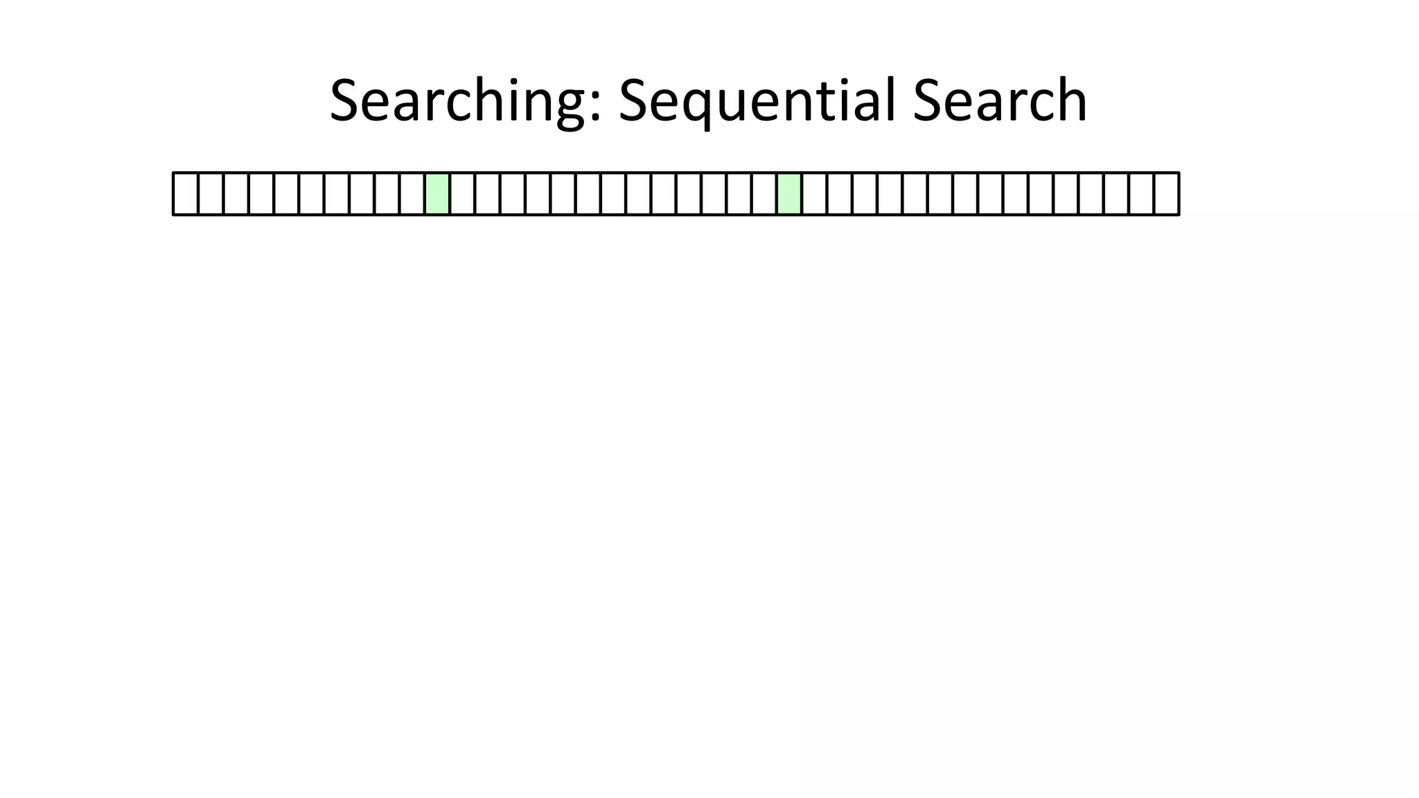
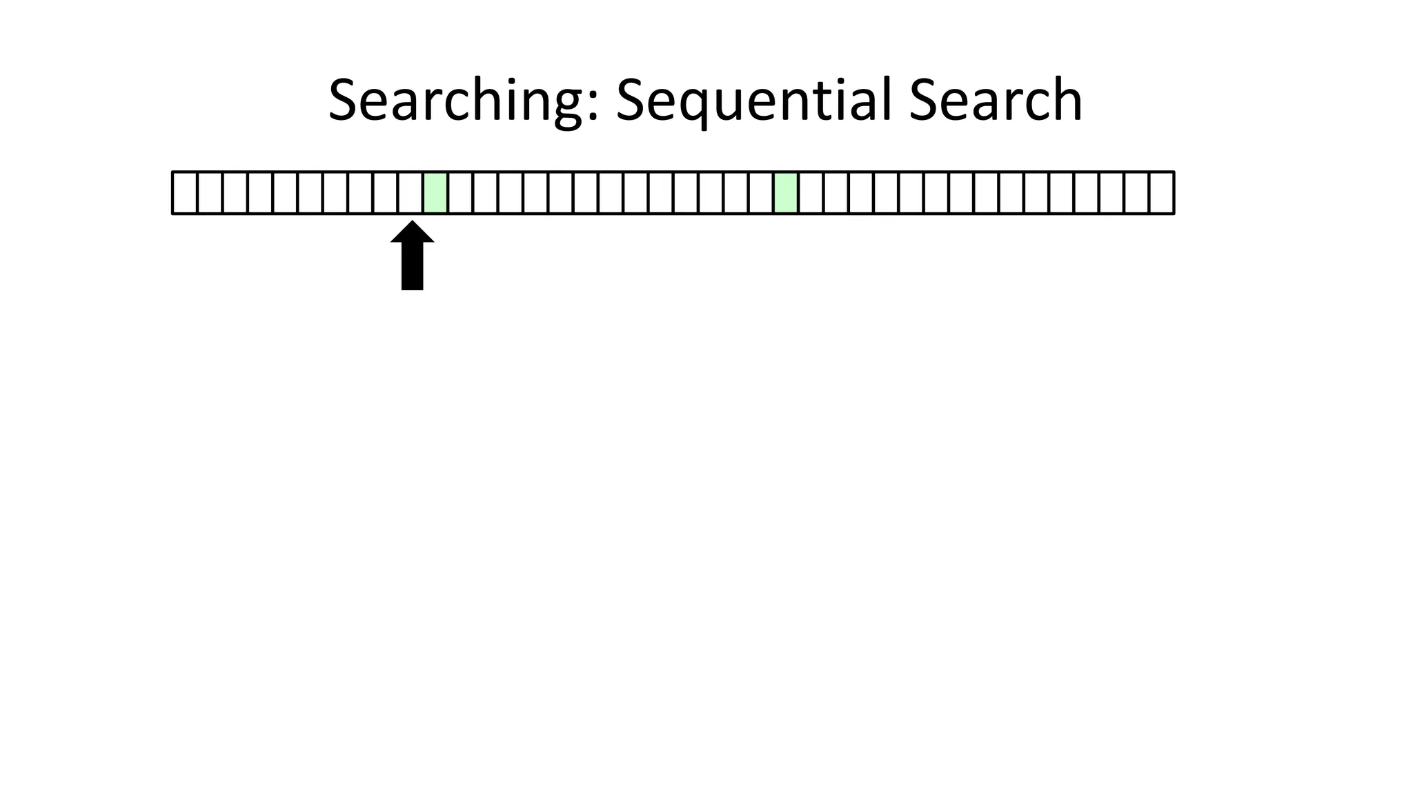
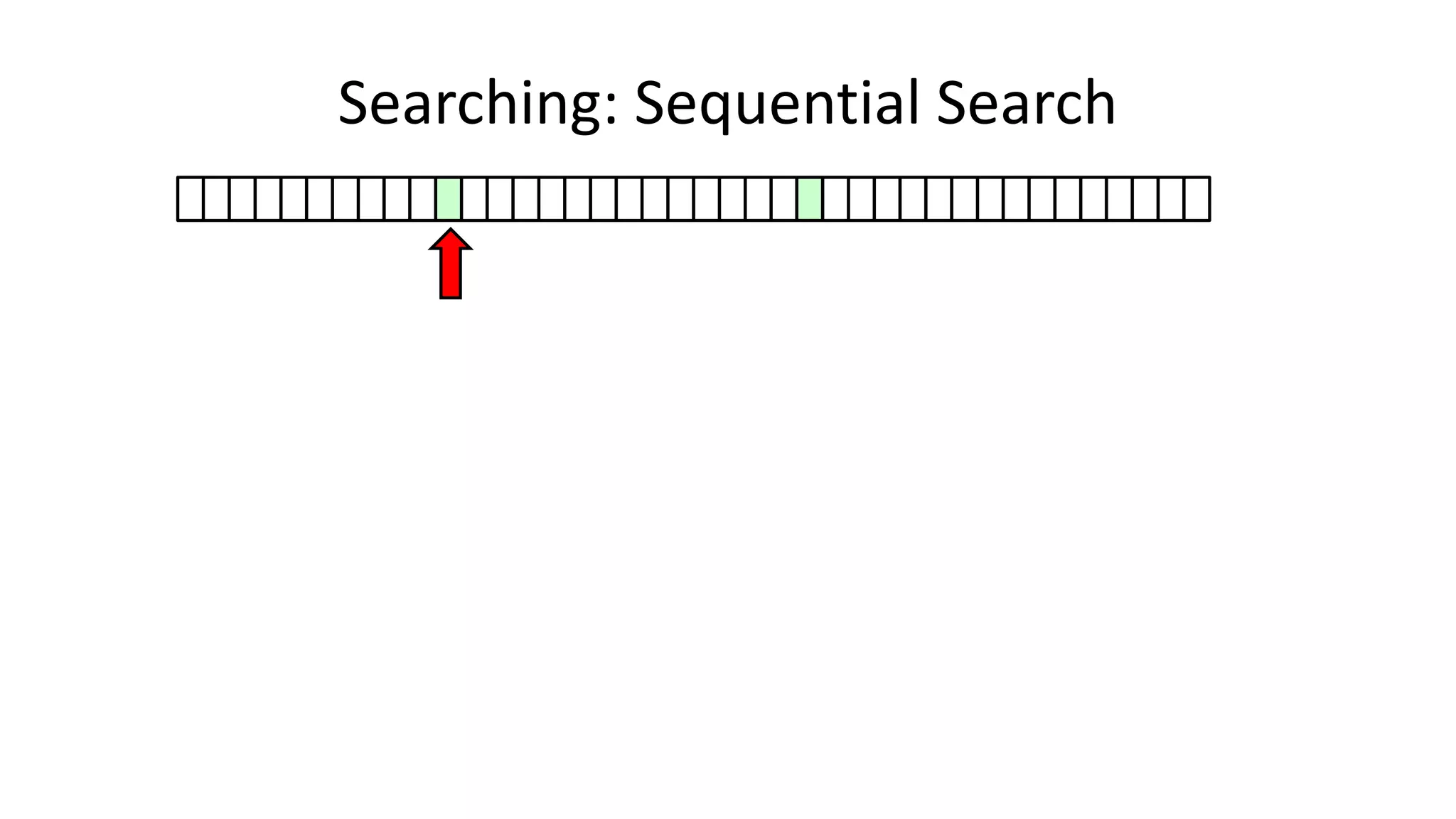
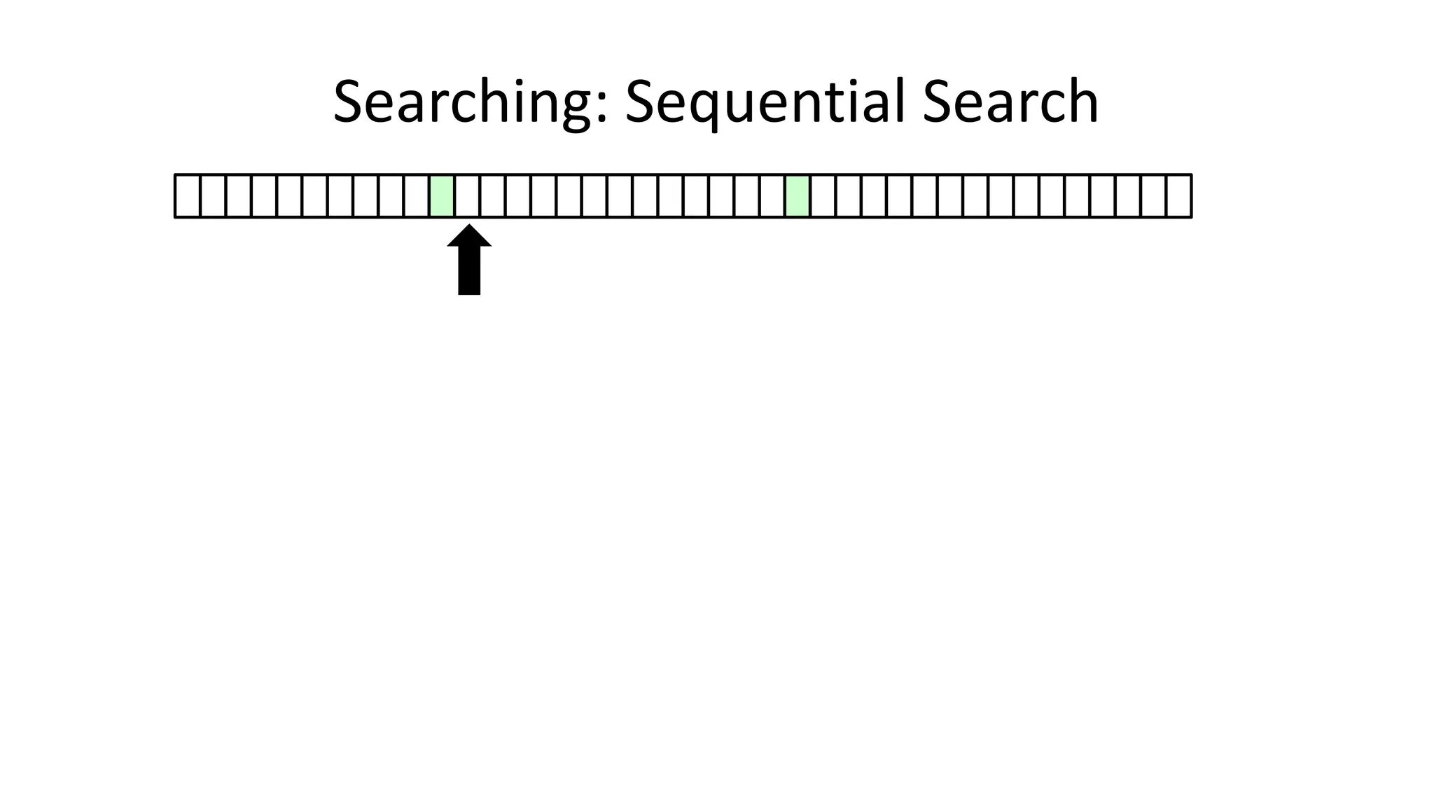
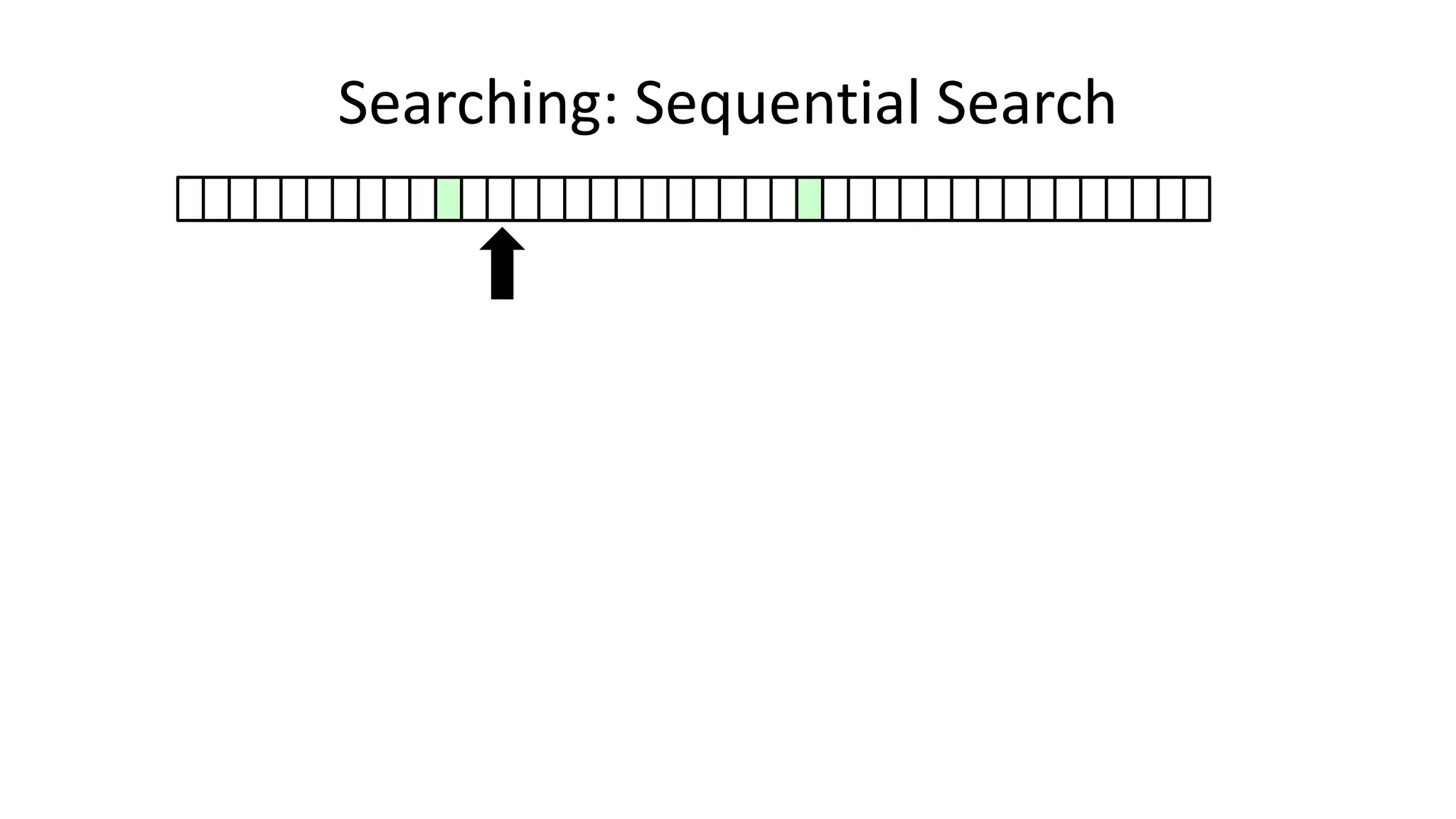
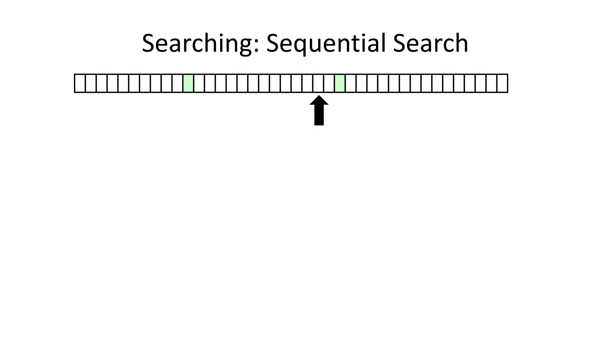
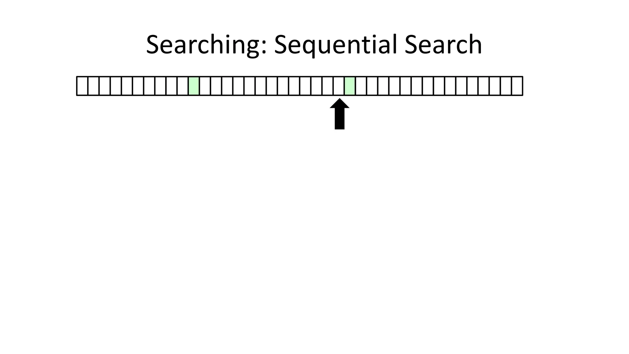
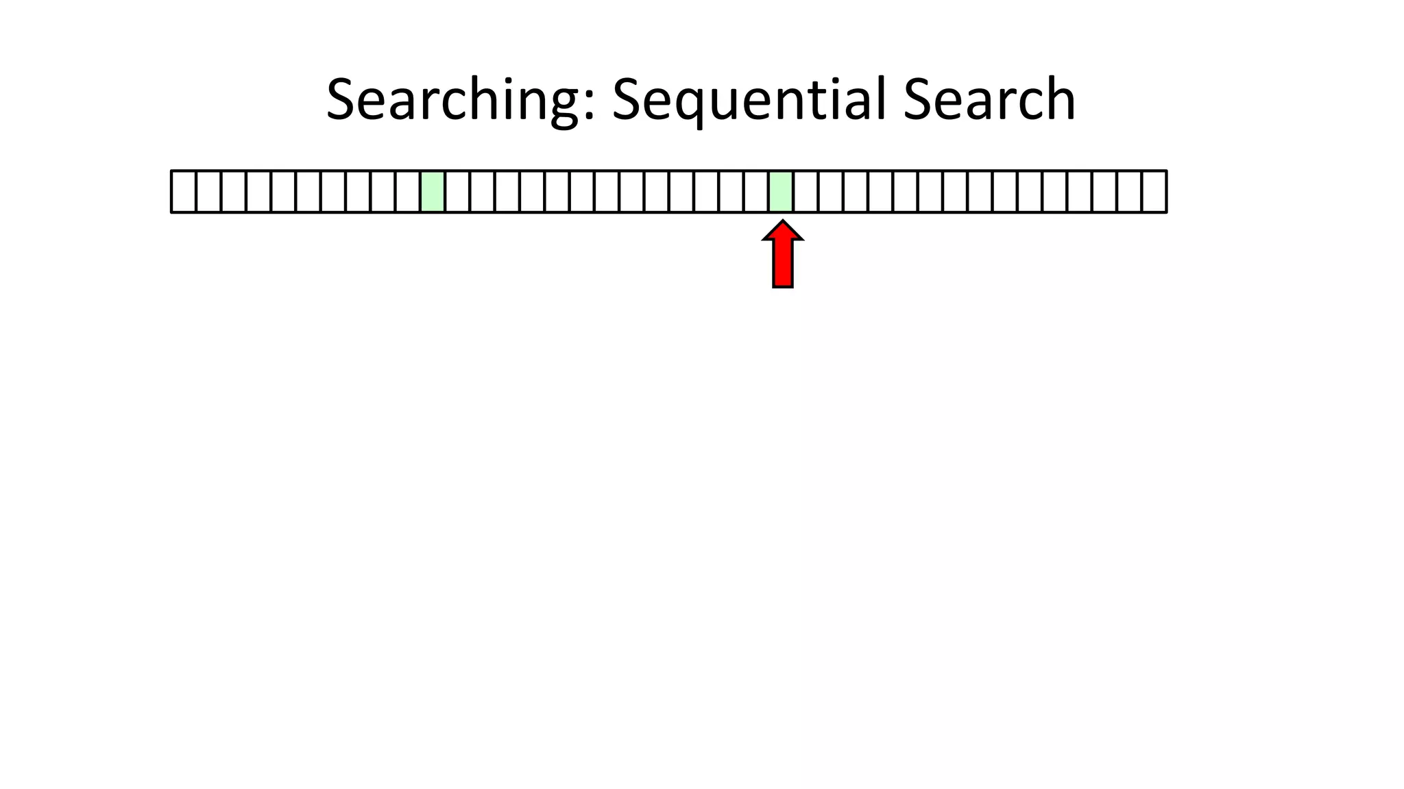
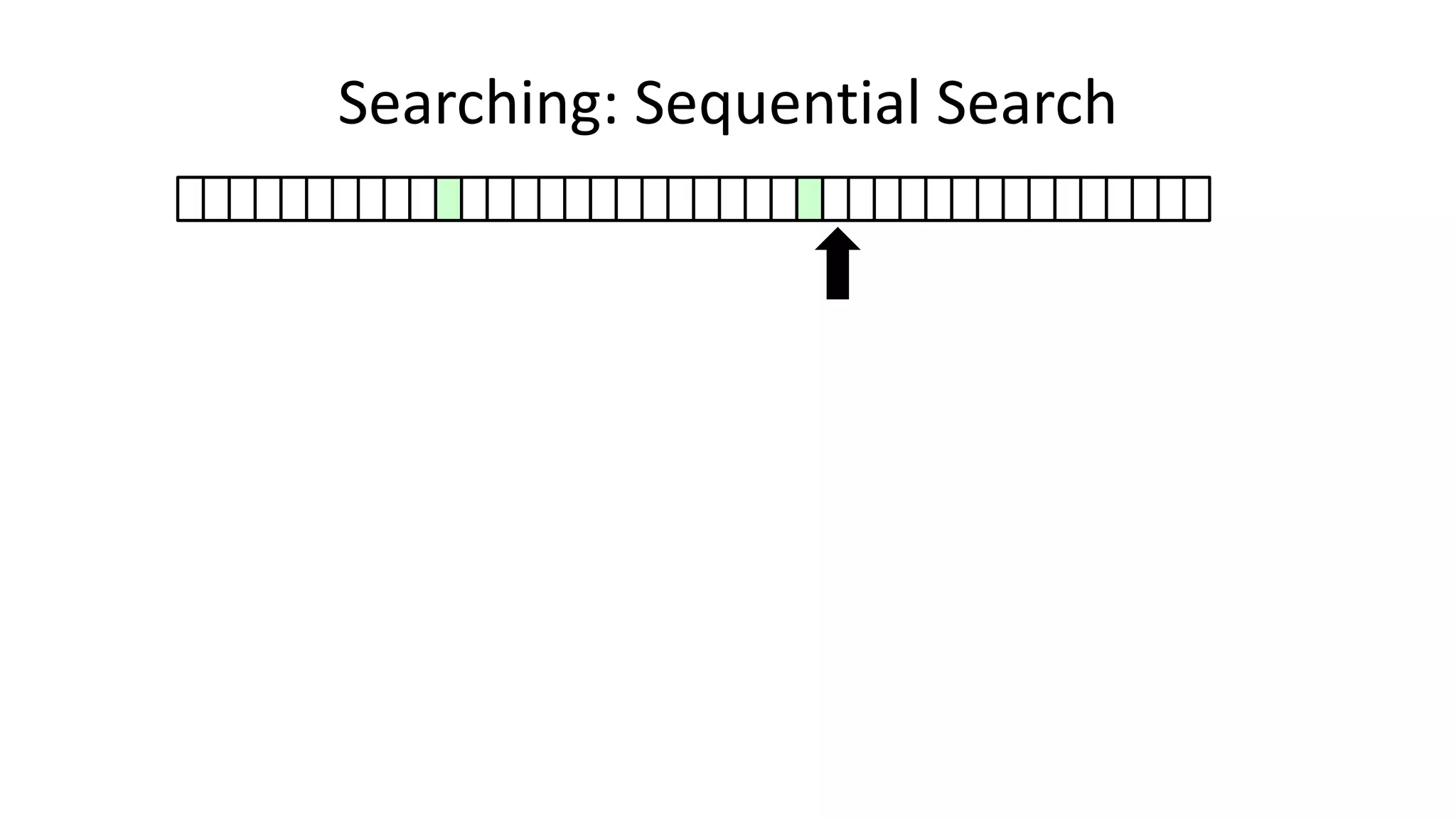
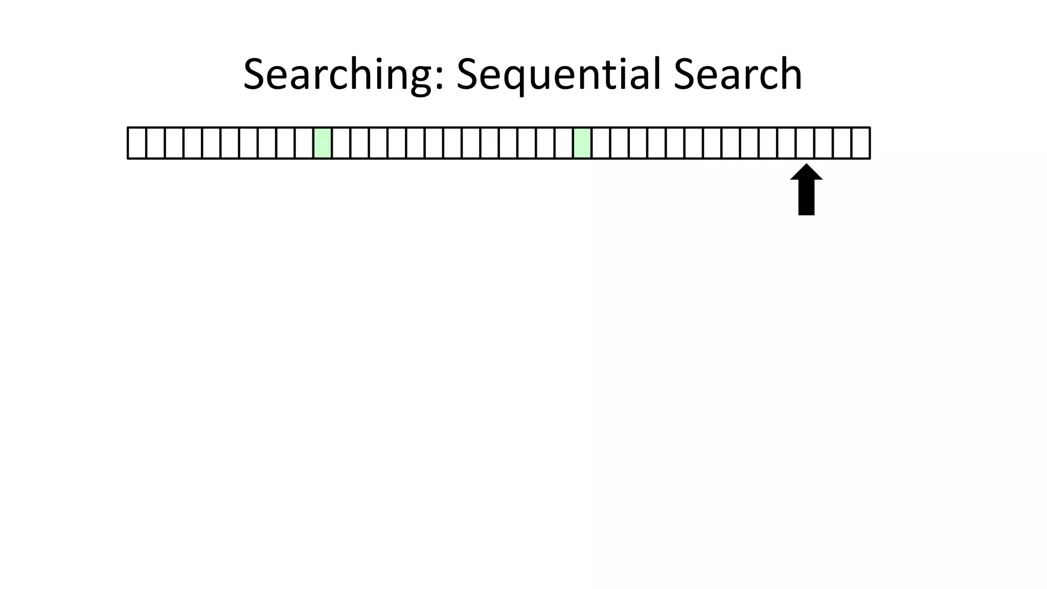
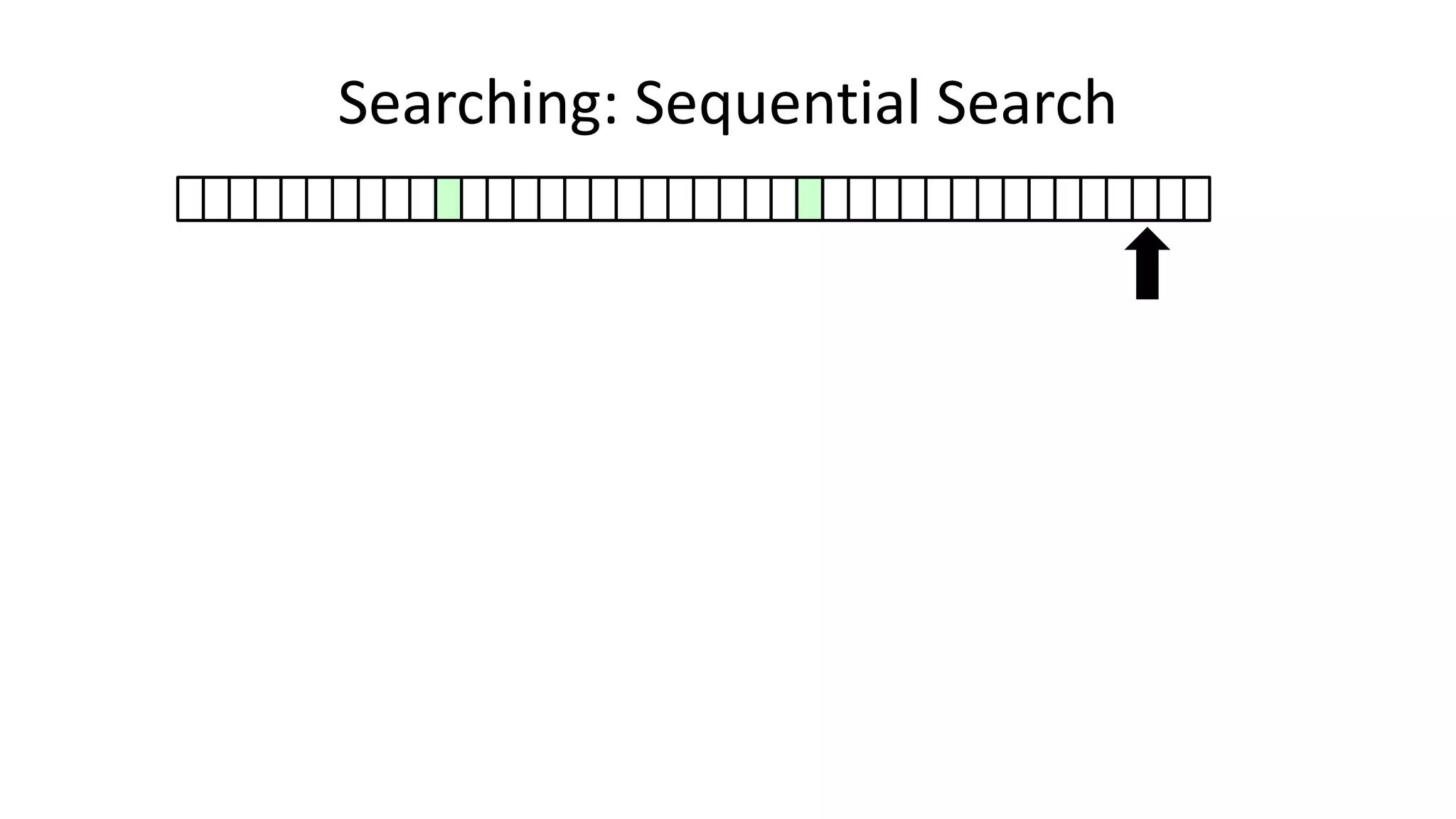
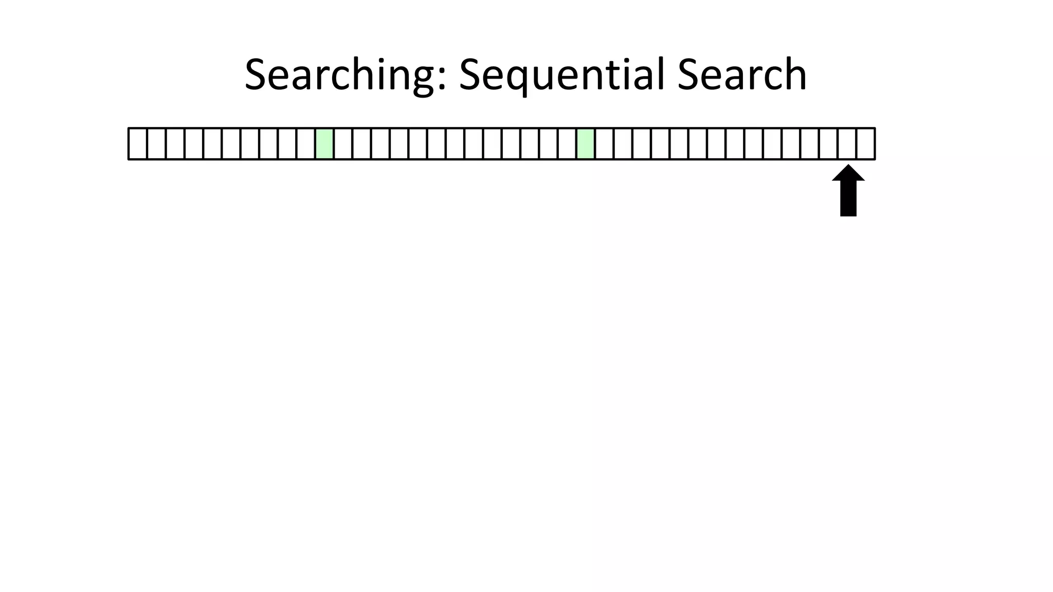
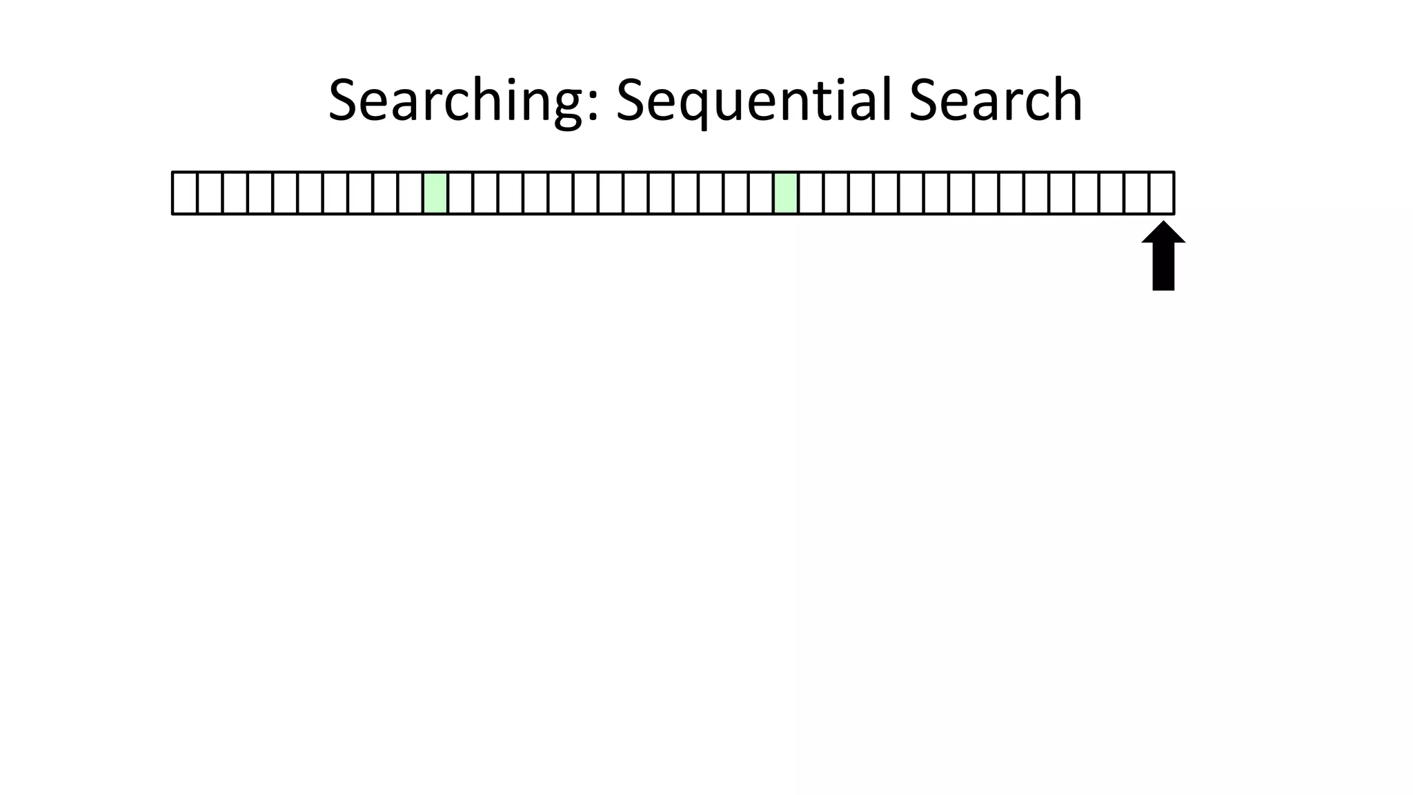
![• Here’s how we could do it:
PROGRAM SequentialSearch:
integer SearchValue <- 18;
integer ArraySize <- 40;
FOR N IN 0 TO ArraySize-1
DO IF Age[N] = SearchValue
THEN PRINT “User “ N “is 18”;
ENDIF;
ENDFOR;
END.
Searching: Sequential Search](https://crownmelresort.com/image.slidesharecdn.com/completecourse-150726101701-lva1-app6892/75/A-complete-course-in-Program-Design-using-Pseudocode-420-2048.jpg)


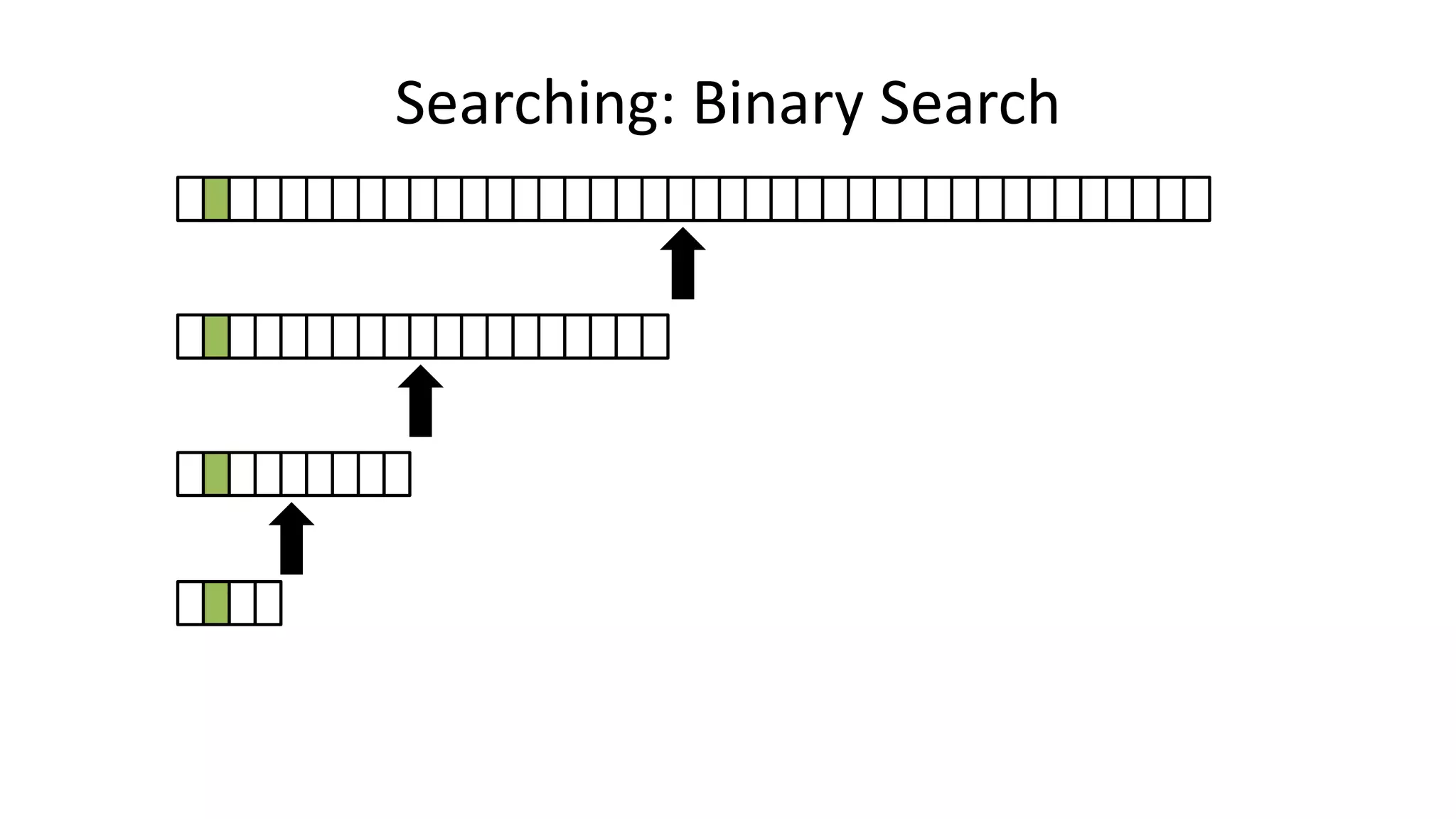
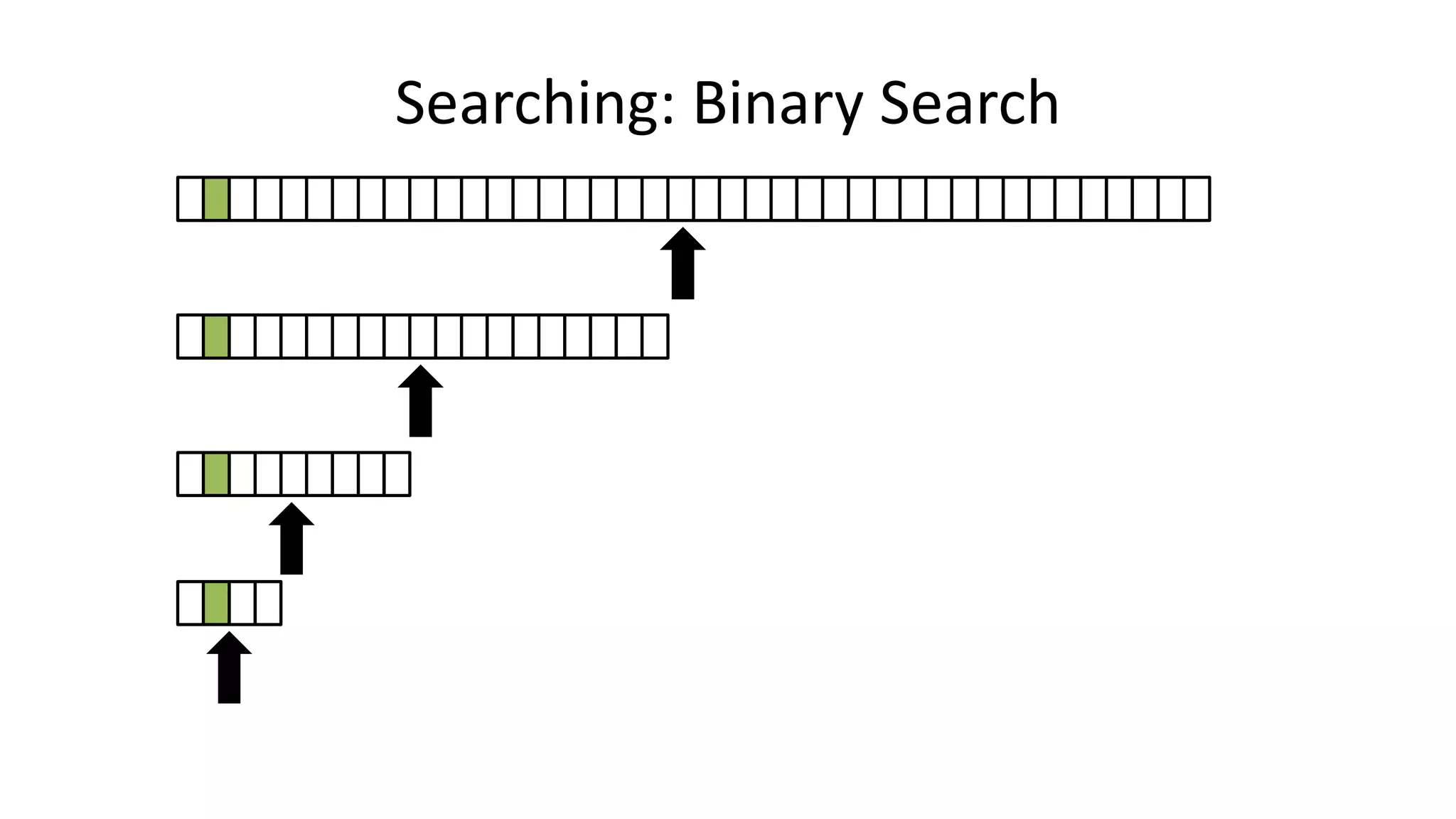
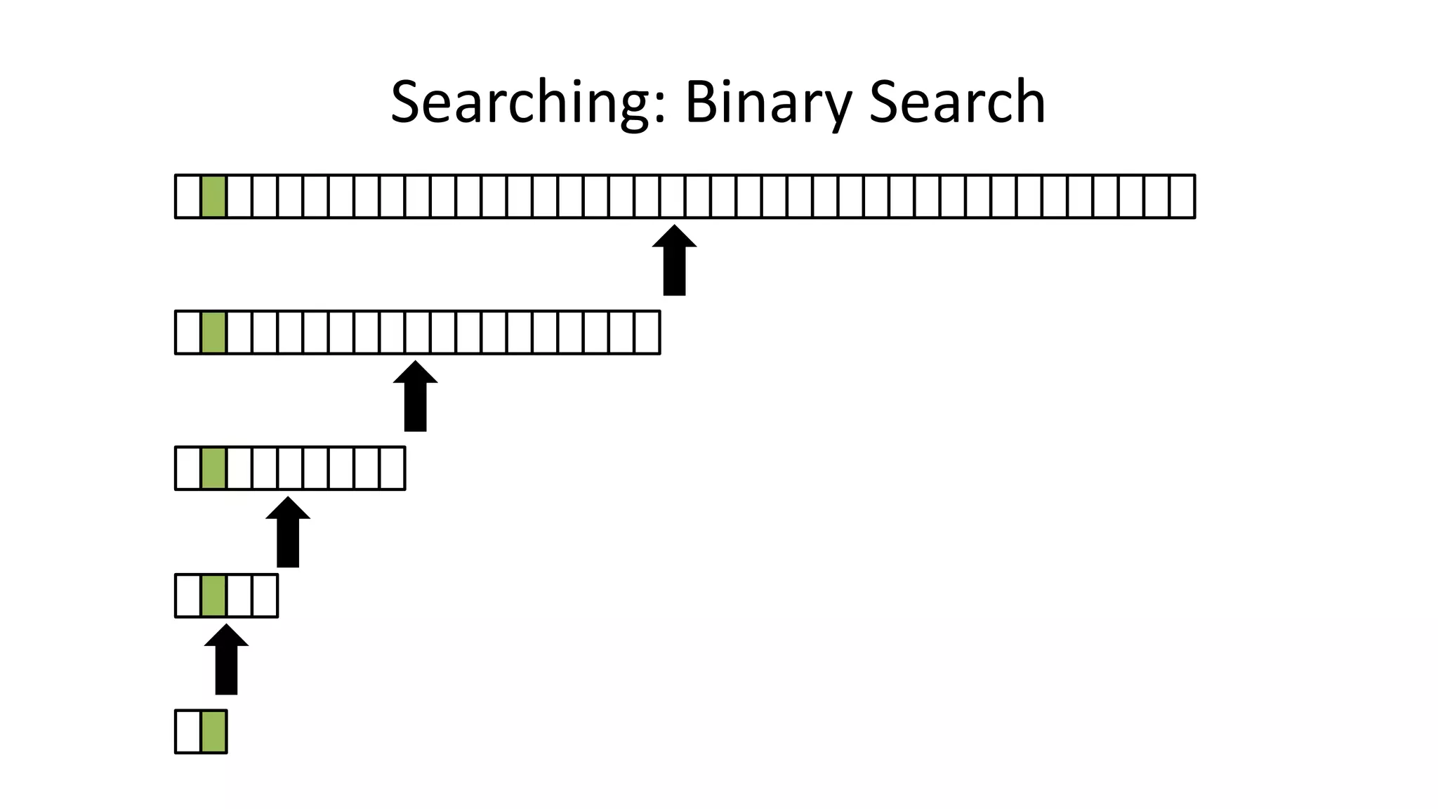
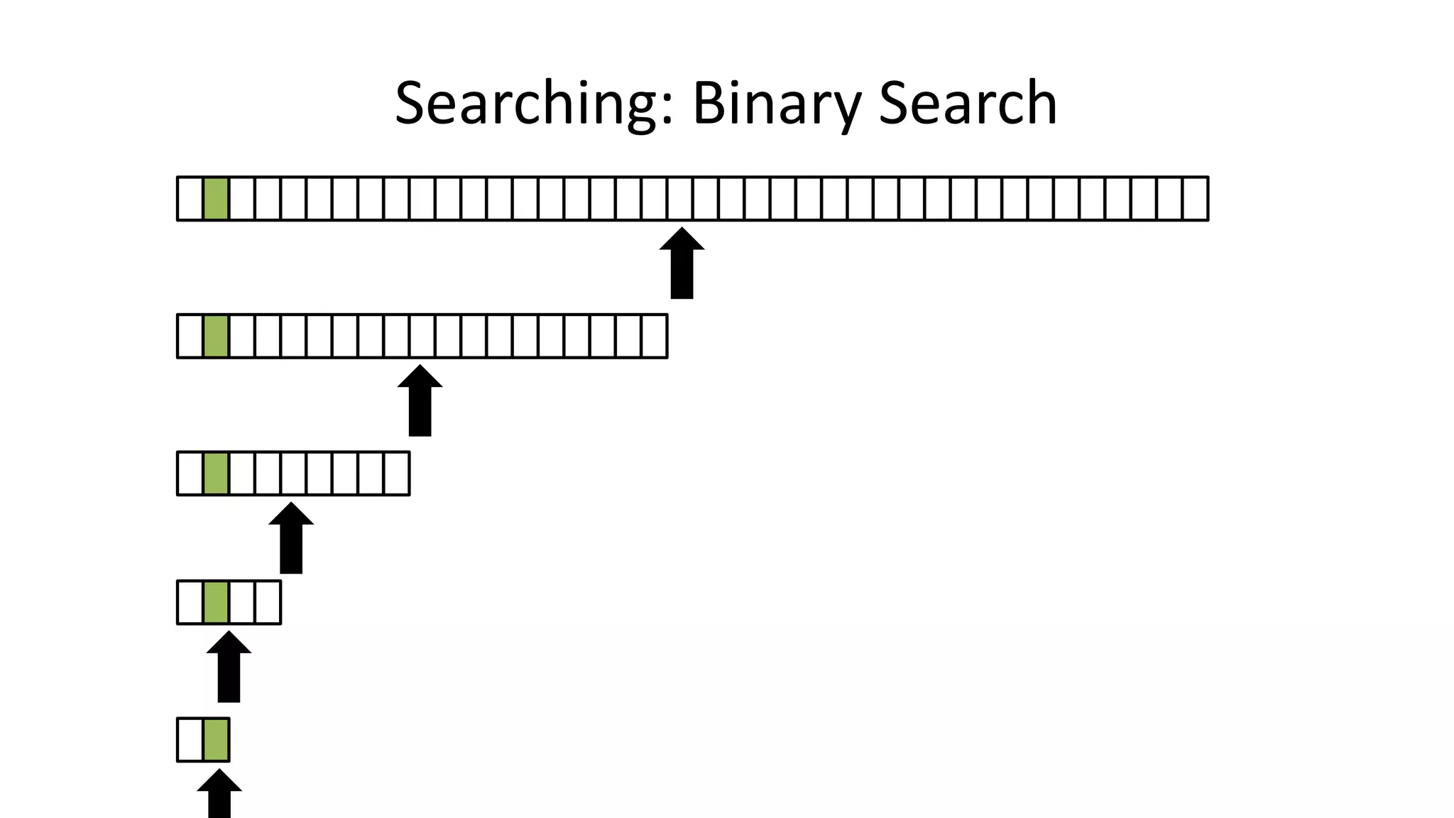
![• If the data is sorted, we can do a BINARY SEARCH
PROGRAM BinarySearch:
integer First <- 0;
integer Last <- 40;
boolean IsFound <- FALSE;
WHILE First <= Last AND IsFound = FALSE
DO Index = (First + Last)/2;
IF Age[Index] = SearchValue
THEN IsFound <- TRUE;
ELSE IF Age[Index] > SearchValue
THEN Last <- Index-1;
ELSE First <- Index+1;
ENDIF;
ENDIF;
ENDWHILE;
END.
Searching: Binary Search](https://crownmelresort.com/image.slidesharecdn.com/completecourse-150726101701-lva1-app6892/75/A-complete-course-in-Program-Design-using-Pseudocode-437-2048.jpg)


![• Here’s how we could do it:
PROGRAM MinimumValue:
integer ArraySize <- 8;
MinValSoFar <- Age[0];
FOR N IN 1 TO ArraySize-1
DO IF MinValSoFar > Age[N]
THEN MinValSoFar <- Age[N];
ENDIF;
ENDFOR;
PRINT MinValSoFar;
END.
Minimum Value in Array](https://crownmelresort.com/image.slidesharecdn.com/completecourse-150726101701-lva1-app6892/75/A-complete-course-in-Program-Design-using-Pseudocode-441-2048.jpg)

![• Here’s how we could do it:
PROGRAM MaximumValue:
integer ArraySize <- 8;
MaxValSoFar <- Age[0];
FOR N IN 1 TO ArraySize-1
DO IF MaxValSoFar < Age[N]
THEN MaxValSoFar <- Age[N];
ENDIF;
ENDFOR;
PRINT MaxValSoFar;
END.
Maximum Value in Array](https://crownmelresort.com/image.slidesharecdn.com/completecourse-150726101701-lva1-app6892/75/A-complete-course-in-Program-Design-using-Pseudocode-443-2048.jpg)

![• Here’s how we could do it:
PROGRAM AverageValue:
integer ArraySize <- 8;
Integer Total <- 0;
FOR N IN 1 TO ArraySize-1
DO Total <- Total + Age[N];
ENDFOR;
PRINT Total/ArraySize;
END.
Average Value in Array](https://crownmelresort.com/image.slidesharecdn.com/completecourse-150726101701-lva1-app6892/75/A-complete-course-in-Program-Design-using-Pseudocode-445-2048.jpg)


![• First Draft
PROGRAM StandardDeviationValue:
integer ArraySize <- 8;
GET AVERAGE OF ARRAY;
TotalSDNum <- 0;
FOR N IN 0 TO ArraySize-1
DO SDNum <-(Age[N]-ArrayAvg)*(Age[N]-ArrayAvg)
TotalSDNum <- TotalSDNum + SDNum;
ENDFOR;
Print SquareRoot(TotalSDNum/ArraySize-1);
END.
Standard Deviation of an Array](https://crownmelresort.com/image.slidesharecdn.com/completecourse-150726101701-lva1-app6892/75/A-complete-course-in-Program-Design-using-Pseudocode-448-2048.jpg)
![• Here’s the final version:
PROGRAM StandardDeviationValue:
integer ArraySize <- 8;
Integer TotalAvg <- 0;
FOR N IN 1 TO ArraySize-1
DO TotalAvg <- TotalAvg + Age[N];
ENDFOR;
AverageValue <- TotalAvg/ArraySize;
TotalSDNum <- 0;
FOR N IN 0 TO ArraySize-1
DO SDNum <-(Age[N]-AverageValue)*(Age[N]- AverageValue)
TotalSDNum <- TotalSDNum + SDNum;
ENDFOR;
Print SquareRoot(TotalSDNum/ArraySize-1);
END.
Standard Deviation of an Array](https://crownmelresort.com/image.slidesharecdn.com/completecourse-150726101701-lva1-app6892/75/A-complete-course-in-Program-Design-using-Pseudocode-449-2048.jpg)


![• Lets look at the swapping bit
– if I wanted to swap two values, the following won’t work:
Age[0] <- Age[1];
Age[1] <- Age[0];
– Why not?
Sorting: Bubble Sort](https://crownmelresort.com/image.slidesharecdn.com/completecourse-150726101701-lva1-app6892/75/A-complete-course-in-Program-Design-using-Pseudocode-460-2048.jpg)
![• Lets assume Age[0]=44, and Age[1]=23, if we do the following:
Age[0] <- Age[1];
Age[1] <- Age[0];
– What happens is:
Age[0] <- Age[1];
Age[1] <- Age[0];
Sorting: Bubble Sort](https://crownmelresort.com/image.slidesharecdn.com/completecourse-150726101701-lva1-app6892/75/A-complete-course-in-Program-Design-using-Pseudocode-461-2048.jpg)
![• Lets assume Age[0]=44, and Age[1]=23, if we do the following:
Age[0] <- Age[1];
Age[1] <- Age[0];
– What happens is:
Age[0] <- Age[1];
Age[1] <- Age[0];
Sorting: Bubble Sort
23](https://crownmelresort.com/image.slidesharecdn.com/completecourse-150726101701-lva1-app6892/75/A-complete-course-in-Program-Design-using-Pseudocode-462-2048.jpg)
![• Lets assume Age[0]=44, and Age[1]=23, if we do the following:
Age[0] <- Age[1];
Age[1] <- Age[0];
– What happens is:
Age[0] <- Age[1];
Age[1] <- Age[0];
Sorting: Bubble Sort
2323](https://crownmelresort.com/image.slidesharecdn.com/completecourse-150726101701-lva1-app6892/75/A-complete-course-in-Program-Design-using-Pseudocode-463-2048.jpg)
![• Lets assume Age[0]=44, and Age[1]=23, if we do the following:
Age[0] <- Age[1];
Age[1] <- Age[0];
– What happens is:
Age[0] <- Age[1];
Age[1] <- Age[0];
Sorting: Bubble Sort
2323
23](https://crownmelresort.com/image.slidesharecdn.com/completecourse-150726101701-lva1-app6892/75/A-complete-course-in-Program-Design-using-Pseudocode-464-2048.jpg)
![• Lets assume Age[0]=44, and Age[1]=23, if we do the following:
Age[0] <- Age[1];
Age[1] <- Age[0];
– What happens is:
Age[0] <- Age[1];
Age[1] <- Age[0];
Sorting: Bubble Sort
2323
2323](https://crownmelresort.com/image.slidesharecdn.com/completecourse-150726101701-lva1-app6892/75/A-complete-course-in-Program-Design-using-Pseudocode-465-2048.jpg)
![• Lets assume Age[0]=44, and Age[1]=23, if we do the following:
Age[0] <- Age[1];
Age[1] <- Age[0];
– What happens is:
Age[0] <- Age[1];
Age[1] <- Age[0];
Sorting: Bubble Sort
2323
2323](https://crownmelresort.com/image.slidesharecdn.com/completecourse-150726101701-lva1-app6892/75/A-complete-course-in-Program-Design-using-Pseudocode-466-2048.jpg)
![• Lets assume Age[0]=44, and Age[1]=23, if we do the following:
Age[0] <- Age[1];
Age[1] <- Age[0];
– What happens is:
Age[0] <- Age[1];
Age[1] <- Age[0];
Sorting: Bubble Sort
2323
2323](https://crownmelresort.com/image.slidesharecdn.com/completecourse-150726101701-lva1-app6892/75/A-complete-course-in-Program-Design-using-Pseudocode-467-2048.jpg)


![• We need an extra variable to make this work:
• Lets call it Temp_Value.
Temp_Value <- Age[1];
Sorting: Bubble Sort](https://crownmelresort.com/image.slidesharecdn.com/completecourse-150726101701-lva1-app6892/75/A-complete-course-in-Program-Design-using-Pseudocode-470-2048.jpg)
![• We need an extra variable to make this work:
• Lets call it Temp_Value.
Temp_Value <- Age[1];
Age[1] <- Age[0];
Sorting: Bubble Sort](https://crownmelresort.com/image.slidesharecdn.com/completecourse-150726101701-lva1-app6892/75/A-complete-course-in-Program-Design-using-Pseudocode-471-2048.jpg)
![• We need an extra variable to make this work:
• Lets call it Temp_Value.
Temp_Value <- Age[1];
Age[1] <- Age[0];
Age[0] <- Temp_Value;
Sorting: Bubble Sort](https://crownmelresort.com/image.slidesharecdn.com/completecourse-150726101701-lva1-app6892/75/A-complete-course-in-Program-Design-using-Pseudocode-472-2048.jpg)
![• We need an extra variable to make this work:
• Lets call it Temp_Value.
Temp_Value <- Age[1];
Age[1] <- Age[0];
Age[0] <- Temp_Value;
Sorting: Bubble Sort
23](https://crownmelresort.com/image.slidesharecdn.com/completecourse-150726101701-lva1-app6892/75/A-complete-course-in-Program-Design-using-Pseudocode-473-2048.jpg)
![• We need an extra variable to make this work:
• Lets call it Temp_Value.
Temp_Value <- Age[1];
Age[1] <- Age[0];
Age[0] <- Temp_Value;
Sorting: Bubble Sort
2323](https://crownmelresort.com/image.slidesharecdn.com/completecourse-150726101701-lva1-app6892/75/A-complete-course-in-Program-Design-using-Pseudocode-474-2048.jpg)
![• We need an extra variable to make this work:
• Lets call it Temp_Value.
Temp_Value <- Age[1];
Age[1] <- Age[0];
Age[0] <- Temp_Value;
Sorting: Bubble Sort
2323
44](https://crownmelresort.com/image.slidesharecdn.com/completecourse-150726101701-lva1-app6892/75/A-complete-course-in-Program-Design-using-Pseudocode-475-2048.jpg)
![• We need an extra variable to make this work:
• Lets call it Temp_Value.
Temp_Value <- Age[1];
Age[1] <- Age[0];
Age[0] <- Temp_Value;
Sorting: Bubble Sort
2323
4444](https://crownmelresort.com/image.slidesharecdn.com/completecourse-150726101701-lva1-app6892/75/A-complete-course-in-Program-Design-using-Pseudocode-476-2048.jpg)
![• We need an extra variable to make this work:
• Lets call it Temp_Value.
Temp_Value <- Age[1];
Age[1] <- Age[0];
Age[0] <- Temp_Value;
Sorting: Bubble Sort
2323
4444
23](https://crownmelresort.com/image.slidesharecdn.com/completecourse-150726101701-lva1-app6892/75/A-complete-course-in-Program-Design-using-Pseudocode-477-2048.jpg)
![• We need an extra variable to make this work:
• Lets call it Temp_Value.
Temp_Value <- Age[1];
Age[1] <- Age[0];
Age[0] <- Temp_Value;
Sorting: Bubble Sort
2323
4444
2323](https://crownmelresort.com/image.slidesharecdn.com/completecourse-150726101701-lva1-app6892/75/A-complete-course-in-Program-Design-using-Pseudocode-478-2048.jpg)
![• We need an extra variable to make this work:
• Lets call it Temp_Value.
Temp_Value <- Age[1];
Age[1] <- Age[0];
Age[0] <- Temp_Value;
Sorting: Bubble Sort
2323
4444
2323](https://crownmelresort.com/image.slidesharecdn.com/completecourse-150726101701-lva1-app6892/75/A-complete-course-in-Program-Design-using-Pseudocode-479-2048.jpg)
![• We need an extra variable to make this work:
• Lets call it Temp_Value.
Temp_Value <- Age[1];
Age[1] <- Age[0];
Age[0] <- Temp_Value;
Sorting: Bubble Sort
2323
4444
2323](https://crownmelresort.com/image.slidesharecdn.com/completecourse-150726101701-lva1-app6892/75/A-complete-course-in-Program-Design-using-Pseudocode-480-2048.jpg)
![• Let’s wrap an IF statement around this:
IF (Age[1] < Age[0])
THEN Temp_Value <- Age[1];
Age[1] <- Age[0];
Age[0] <- Temp_Value;
ENDIF;
Sorting: Bubble Sort](https://crownmelresort.com/image.slidesharecdn.com/completecourse-150726101701-lva1-app6892/75/A-complete-course-in-Program-Design-using-Pseudocode-481-2048.jpg)
![• And in general:
IF (Age[N+1] < Age[N])
THEN Temp_Value <- Age[N+1];
Age[N+1] <- Age[N];
Age[N] <- Temp_Value;
ENDIF;
Sorting: Bubble Sort](https://crownmelresort.com/image.slidesharecdn.com/completecourse-150726101701-lva1-app6892/75/A-complete-course-in-Program-Design-using-Pseudocode-482-2048.jpg)
![• Let’s replace “N” with “Index”
IF (Age[Index+1] < Age[Index])
THEN Temp_Value <- Age[Index+1];
Age[Index+1] <- Age[Index];
Age[Index] <- Temp_Value;
ENDIF;
Sorting: Bubble Sort](https://crownmelresort.com/image.slidesharecdn.com/completecourse-150726101701-lva1-app6892/75/A-complete-course-in-Program-Design-using-Pseudocode-483-2048.jpg)
![• To get from one end of the array to another:
FOR Index IN 0 TO N-2
DO IF (Age[Index+1] < Age[Index])
THEN Temp_Value <- Age[Index+1];
Age[Index+1] <- Age[Index];
Age[Index] <- Temp_Value;
ENDIF;
ENDFOR;
Sorting: Bubble Sort](https://crownmelresort.com/image.slidesharecdn.com/completecourse-150726101701-lva1-app6892/75/A-complete-course-in-Program-Design-using-Pseudocode-484-2048.jpg)


![• So we need two loops:
FOR Outer-Index IN 0 TO N-1
DO FOR Index IN 0 TO N-2
DO IF (Age[Index+1] < Age[Index])
THEN Temp_Value <- Age[Index+1];
Age[Index+1] <- Age[Index];
Age[Index] <- Temp_Value;
ENDIF;
ENDFOR;
ENDFOR;
Sorting: Bubble Sort](https://crownmelresort.com/image.slidesharecdn.com/completecourse-150726101701-lva1-app6892/75/A-complete-course-in-Program-Design-using-Pseudocode-588-2048.jpg)
![PROGRAM BubbleSort:
Integer Age[8] <- {44,23,42,33,16,54,34,18};
FOR Outer-Index IN 0 TO N-1
DO FOR Index IN 0 TO N-2
DO IF (Age[Index+1] < Age[Index])
THEN Temp_Value <- Age[Index+1];
Age[Index+1] <- Age[Index];
Age[Index] <- Temp_Value;
ENDIF;
ENDFOR;
ENDFOR;
END.
Sorting: Bubble Sort](https://crownmelresort.com/image.slidesharecdn.com/completecourse-150726101701-lva1-app6892/75/A-complete-course-in-Program-Design-using-Pseudocode-589-2048.jpg)


![PROGRAM BubbleSort:
Integer Age[8] <- {44,23,42,33,16,54,34,18};
FOR Outer-Index IN 0 TO N-1
DO FOR Index IN 0 TO N-2
DO IF (Age[Index+1] < Age[Index])
THEN Temp_Value <- Age[Index+1];
Age[Index+1] <- Age[Index];
Age[Index] <- Temp_Value;
ENDIF;
ENDFOR;
ENDFOR;
END.
Sorting: Bubble Sort](https://crownmelresort.com/image.slidesharecdn.com/completecourse-150726101701-lva1-app6892/75/A-complete-course-in-Program-Design-using-Pseudocode-594-2048.jpg)


![PROGRAM BubbleSort:
Integer Age[8] <- {44,23,42,33,16,54,34,18};
ReducingIndex <- N-2;
FOR Outer-Index IN 0 TO N-1
DO FOR Index IN 0 TO ReducingIndex
DO IF (Age[Index+1] < Age[Index])
THEN Temp_Value <- Age[Index+1];
Age[Index+1] <- Age[Index];
Age[Index] <- Temp_Value;
ENDIF;
ENDFOR;
ReducingIndex <- ReducingIndex – 1;
ENDFOR;
END.
Sorting: Bubble Sort](https://crownmelresort.com/image.slidesharecdn.com/completecourse-150726101701-lva1-app6892/75/A-complete-course-in-Program-Design-using-Pseudocode-606-2048.jpg)
![PROGRAM BubbleSort:
Integer Age[8] <- {44,23,42,33,16,54,34,18};
ReducingIndex <- N-2;
FOR Outer-Index IN 0 TO N-1
DO FOR Index IN 0 TO ReducingIndex
DO IF (Age[Index+1] < Age[Index])
THEN Temp_Value <- Age[Index+1];
Age[Index+1] <- Age[Index];
Age[Index] <- Temp_Value;
ENDIF;
ENDFOR;
ReducingIndex <- ReducingIndex – 1;
ENDFOR;
END.
Sorting: Bubble Sort](https://crownmelresort.com/image.slidesharecdn.com/completecourse-150726101701-lva1-app6892/75/A-complete-course-in-Program-Design-using-Pseudocode-607-2048.jpg)

![Sorting: Bubble SortPROGRAM BubbleSort:
Integer Age[8] <- {44,23,42,33,16,54,34,18};
ReducingIndex <- N-2;
DidSwap <- FALSE;
FOR Outer-Index IN 0 TO N-1
DO FOR Index IN 0 TO ReducingIndex
DO IF (Age[Index+1] < Age[Index])
THEN Temp_Value <- Age[Index+1];
Age[Index+1] <- Age[Index];
Age[Index] <- Temp_Value;
DidSwap <- TRUE;
ENDIF;
ENDFOR;
ReducingIndex <- ReducingIndex – 1;
IF (DidSwap = FALSE)
THEN EXIT;
ENDIF;
ENDFOR;
END.](https://crownmelresort.com/image.slidesharecdn.com/completecourse-150726101701-lva1-app6892/75/A-complete-course-in-Program-Design-using-Pseudocode-609-2048.jpg)
![PROGRAM BubbleSort:
Integer Age[8] <- {44,23,42,33,16,54,34,18};
ReducingIndex <- N-2;
DidSwap <- FALSE;
FOR Outer-Index IN 0 TO N-1
DO FOR Index IN 0 TO ReducingIndex
DO IF (Age[Index+1] < Age[Index])
THEN Temp_Value <- Age[Index+1];
Age[Index+1] <- Age[Index];
Age[Index] <- Temp_Value;
DidSwap <- TRUE;
ENDIF;
ENDFOR;
ReducingIndex <- ReducingIndex – 1;
IF (DidSwap = FALSE)
THEN EXIT;
ENDIF;
ENDFOR;
END.
Sorting: Bubble Sort](https://crownmelresort.com/image.slidesharecdn.com/completecourse-150726101701-lva1-app6892/75/A-complete-course-in-Program-Design-using-Pseudocode-610-2048.jpg)

![MODULE SWAP[A,B]:
Integer Temp_Value
Temp_Value <- B;
B <- A;
A <- Temp_Value;
RETURN A, B;
END.
Sorting: Bubble Sort](https://crownmelresort.com/image.slidesharecdn.com/completecourse-150726101701-lva1-app6892/75/A-complete-course-in-Program-Design-using-Pseudocode-612-2048.jpg)
![PROGRAM BubbleSort:
Integer Age[8] <- {44,23,42,33,16,54,34,18};
ReducingIndex <- N-2;
DidSwap <- FALSE;
FOR Outer-Index IN 0 TO N-1
DO FOR Index IN 0 TO ReducingIndex
DO IF (Age[Index+1] < Age[Index])
THEN Temp_Value <- Age[Index+1];
Age[Index+1] <- Age[Index];
Age[Index] <- Temp_Value;
DidSwap <- TRUE;
ENDIF;
ENDFOR;
ReducingIndex <- ReducingIndex – 1;
IF (DidSwap = FALSE)
THEN EXIT;
ENDIF;
ENDFOR;
END.
Sorting: Bubble Sort](https://crownmelresort.com/image.slidesharecdn.com/completecourse-150726101701-lva1-app6892/75/A-complete-course-in-Program-Design-using-Pseudocode-613-2048.jpg)
![PROGRAM BubbleSort:
Integer Age[8] <- {44,23,42,33,16,54,34,18};
ReducingIndex <- N-2;
DidSwap <- FALSE;
FOR Outer-Index IN 0 TO N-1
DO FOR Index IN 0 TO ReducingIndex
DO IF (Age[Index+1] < Age[Index])
THEN Temp_Value <- Age[Index+1];
Age[Index+1] <- Age[Index];
Age[Index] <- Temp_Value;
DidSwap <- TRUE;
ENDIF;
ENDFOR;
ReducingIndex <- ReducingIndex – 1;
IF (DidSwap = FALSE)
THEN EXIT;
ENDIF;
ENDFOR;
END.
Sorting: Bubble Sort](https://crownmelresort.com/image.slidesharecdn.com/completecourse-150726101701-lva1-app6892/75/A-complete-course-in-Program-Design-using-Pseudocode-614-2048.jpg)
![PROGRAM BubbleSort:
Integer Age[8] <- {44,23,42,33,16,54,34,18};
ReducingIndex <- N-2;
DidSwap <- FALSE;
FOR Outer-Index IN 0 TO N-1
DO FOR Index IN 0 TO ReducingIndex
DO IF (Age[Index+1] < Age[Index])
THEN SWAP(Age[Index], Age[Index+1];
DidSwap <- TRUE;
ENDIF;
ENDFOR;
ReducingIndex <- ReducingIndex – 1;
IF (DidSwap = FALSE)
THEN EXIT;
ENDIF;
ENDFOR;
END.
Sorting: Bubble Sort](https://crownmelresort.com/image.slidesharecdn.com/completecourse-150726101701-lva1-app6892/75/A-complete-course-in-Program-Design-using-Pseudocode-615-2048.jpg)


![Sorting: Selection Sort
• So we know we only have to swap if the value is not already in
the correct location.
• This will look a little something like this:
IF (MinValueLocation != CurrentLocation)
THEN Swap(Age[CurrentLocation], Age[MinValueLocation];
ENDIF;](https://crownmelresort.com/image.slidesharecdn.com/completecourse-150726101701-lva1-app6892/75/A-complete-course-in-Program-Design-using-Pseudocode-644-2048.jpg)
![• We will find the minimum value in the list using something like
the following:
MinValueLocation <- 0;
FOR Index IN IncreasingCount TO N-1
DO IF (Age[Index] < Age[MinValueLocation])
THEN MinValueLocation <- Index;
ENDIF;
ENDFOR;
Sorting: Selection Sort](https://crownmelresort.com/image.slidesharecdn.com/completecourse-150726101701-lva1-app6892/75/A-complete-course-in-Program-Design-using-Pseudocode-645-2048.jpg)

![PROGRAM SelectionSort:
Integer Age[8] <- {44,23,42,33,16,54,34,18};
FOR Outer-Index IN 0 TO N-1
MinValueLocation <- Outer-Index;
FOR Index IN Outer-Index+1 TO N-1
DO IF (Age[Index] < Age[MinValueLocation])
THEN MinValueLocation <- Index;
ENDIF;
ENDFOR;
IF (MinValueLocation != Outer-Index)
THEN Swap(Age[Outer-Index], Age[MinValueLocation]);
ENDIF;
ENDFOR;
END.
Sorting: Selection Sort](https://crownmelresort.com/image.slidesharecdn.com/completecourse-150726101701-lva1-app6892/75/A-complete-course-in-Program-Design-using-Pseudocode-647-2048.jpg)


![Arrays
• We declare a multi-dimensional array as follows:
• Integer Age[8][8];](https://crownmelresort.com/image.slidesharecdn.com/completecourse-150726101701-lva1-app6892/75/A-complete-course-in-Program-Design-using-Pseudocode-659-2048.jpg)


![Arrays
• So if I do:
• PRINT Matrix[0][0];
• We will get:
• 45](https://crownmelresort.com/image.slidesharecdn.com/completecourse-150726101701-lva1-app6892/75/A-complete-course-in-Program-Design-using-Pseudocode-664-2048.jpg)
![Arrays
• So if I do:
• PRINT Matrix[2][0];
• We will get:
• 55](https://crownmelresort.com/image.slidesharecdn.com/completecourse-150726101701-lva1-app6892/75/A-complete-course-in-Program-Design-using-Pseudocode-665-2048.jpg)
![Arrays
• So if I do:
• PRINT Matrix[0][2];
• We will get:
• 34](https://crownmelresort.com/image.slidesharecdn.com/completecourse-150726101701-lva1-app6892/75/A-complete-course-in-Program-Design-using-Pseudocode-666-2048.jpg)
![Arrays
• So if I do:
• PRINT Matrix[7][7];
• We will get:
• 23](https://crownmelresort.com/image.slidesharecdn.com/completecourse-150726101701-lva1-app6892/75/A-complete-course-in-Program-Design-using-Pseudocode-667-2048.jpg)
![Arrays
• So if I do:
• Matrix[5][4] <- 43;
• We will get:
• 67 changed to 43](https://crownmelresort.com/image.slidesharecdn.com/completecourse-150726101701-lva1-app6892/75/A-complete-course-in-Program-Design-using-Pseudocode-668-2048.jpg)

![Arrays
PROGRAM Add1ToMartix:
FOR N IN 0 TO 7
FOR M IN 0 TO 7
DO Matrix[N][M] <- Matrix [N][M] + 1;
ENDFOR;
ENDFOR;
END.](https://crownmelresort.com/image.slidesharecdn.com/completecourse-150726101701-lva1-app6892/75/A-complete-course-in-Program-Design-using-Pseudocode-670-2048.jpg)
![Arrays
Or:
PROGRAM Add1ToMartix:
FOR ROW IN 0 TO 7
FOR COLUMN IN 0 TO 7
DO Matrix[ROW][COLUMN] <- Matrix [ROW][COLUMN] + 1;
ENDFOR;
ENDFOR;
END.](https://crownmelresort.com/image.slidesharecdn.com/completecourse-150726101701-lva1-app6892/75/A-complete-course-in-Program-Design-using-Pseudocode-671-2048.jpg)

![Arrays
PROGRAM TotalOfMatrix:
integer Total <- 0;
FOR N IN 0 TO 7
FOR M IN 0 TO 7
DO Total <- Total + Matrix[N][M];
ENDFOR;
ENDFOR;
END.](https://crownmelresort.com/image.slidesharecdn.com/completecourse-150726101701-lva1-app6892/75/A-complete-course-in-Program-Design-using-Pseudocode-673-2048.jpg)

![Arrays
• We can create a 3D array: Array[N][N][N]
• We can create a 4D array: Array[N][N][N][N]
• We can create a 5D array: Array[N][N][N][N][N]
• etc.](https://crownmelresort.com/image.slidesharecdn.com/completecourse-150726101701-lva1-app6892/75/A-complete-course-in-Program-Design-using-Pseudocode-675-2048.jpg)


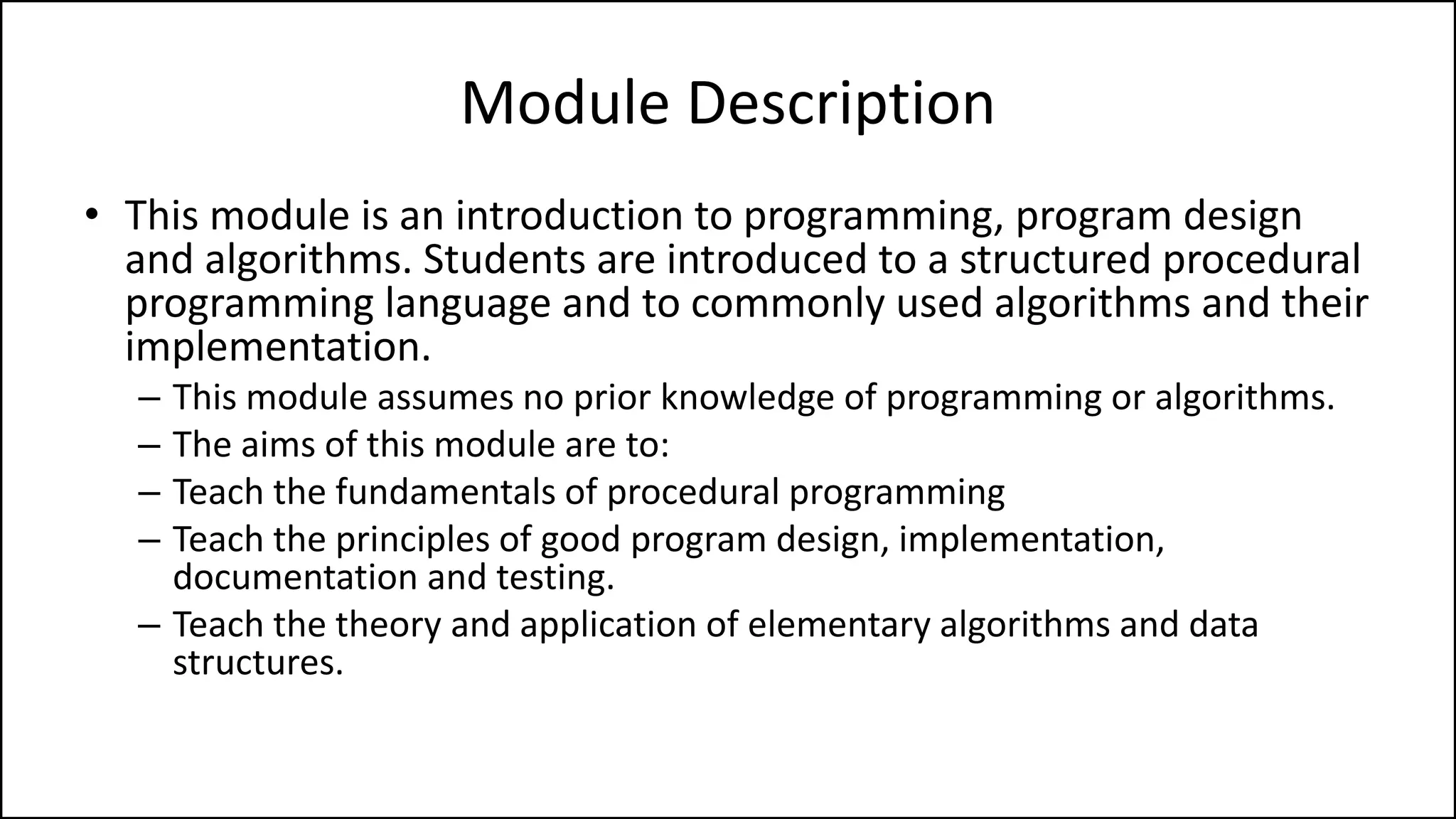
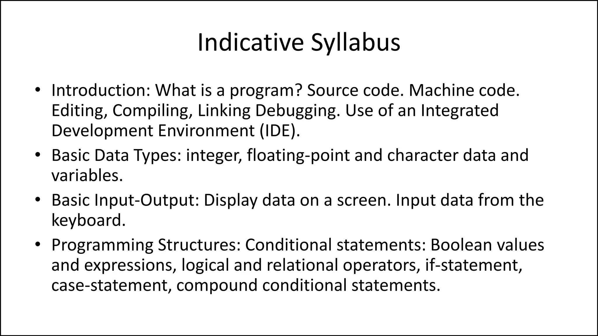
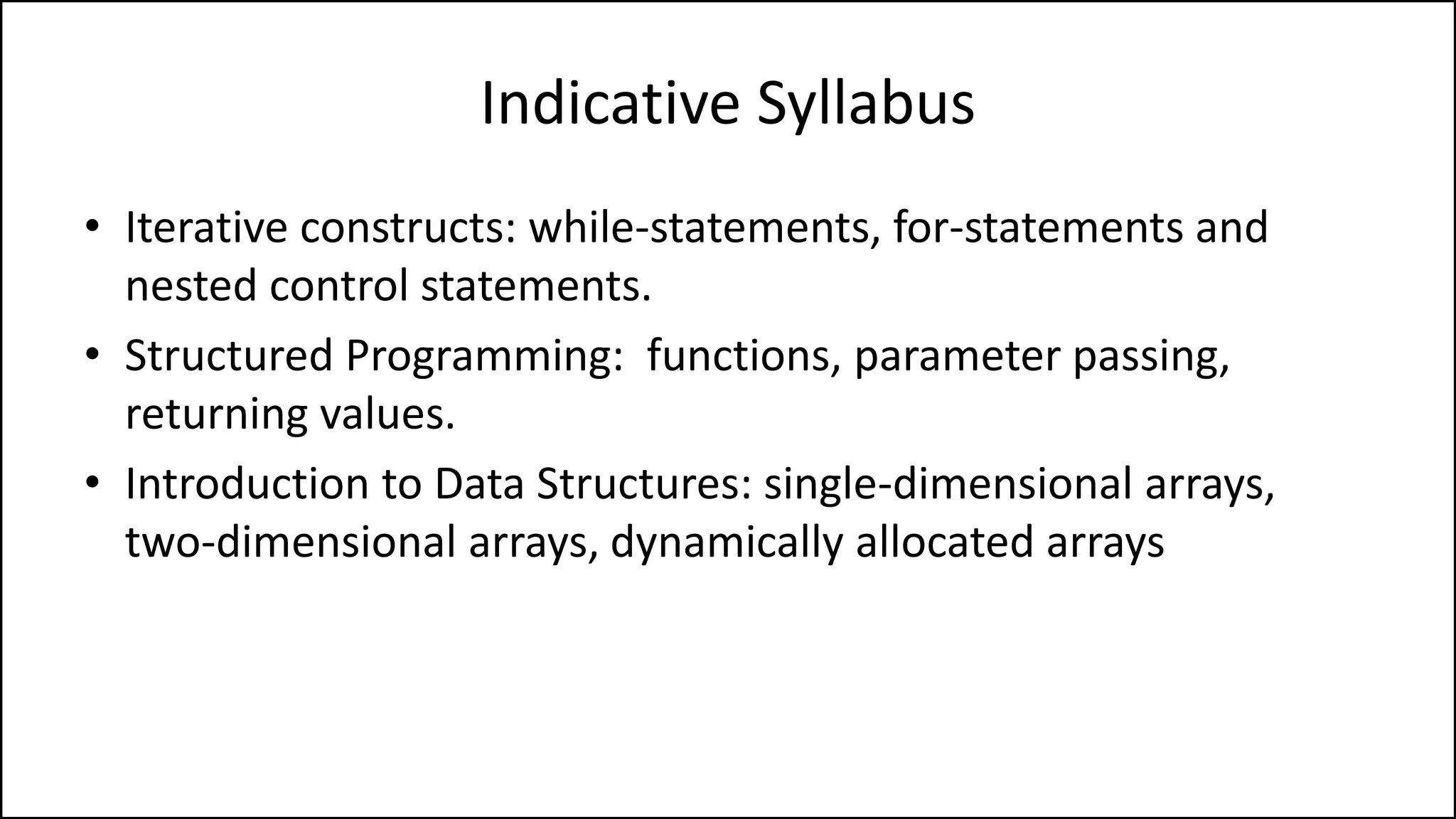
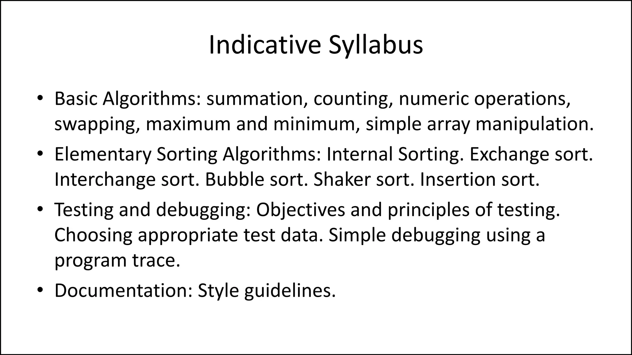
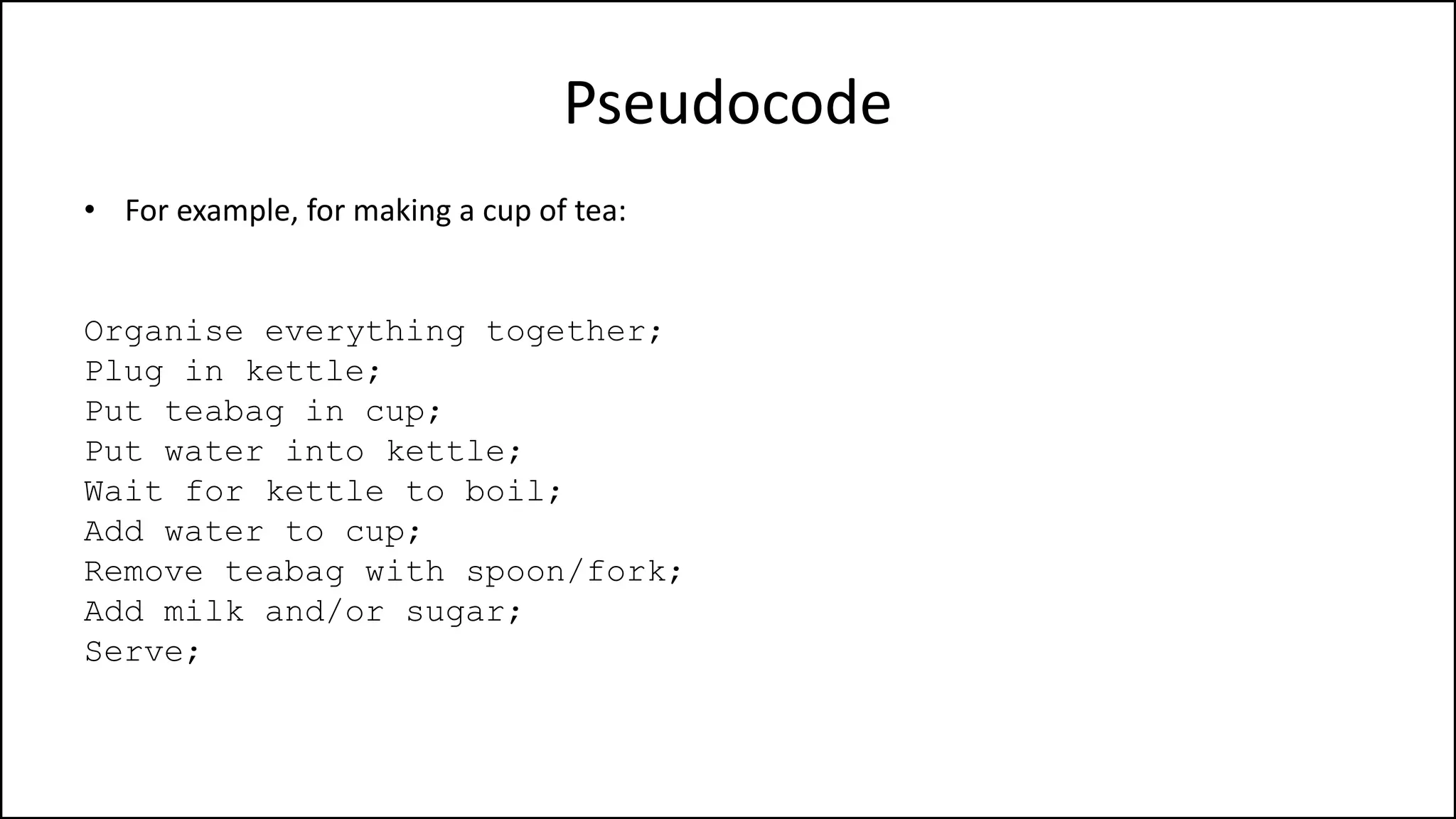
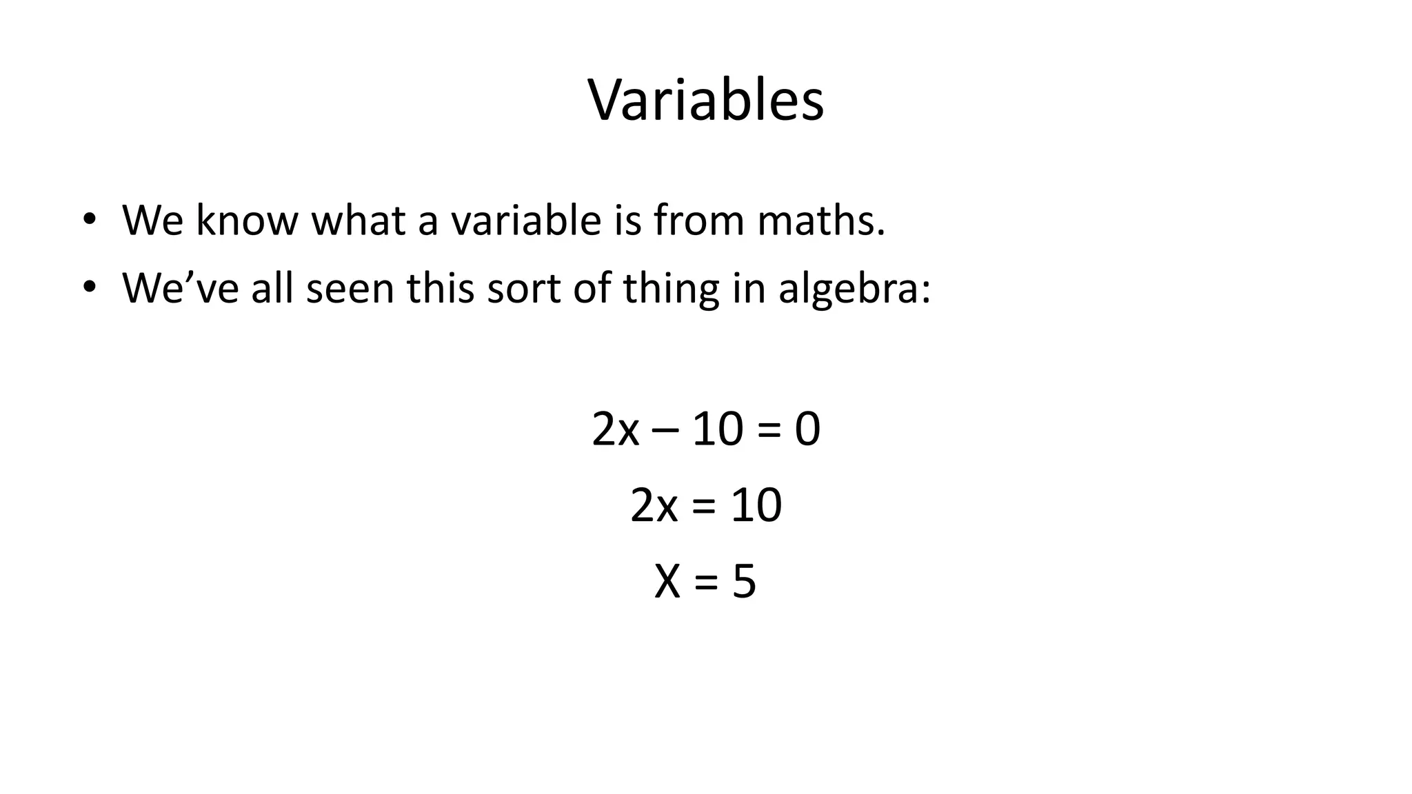
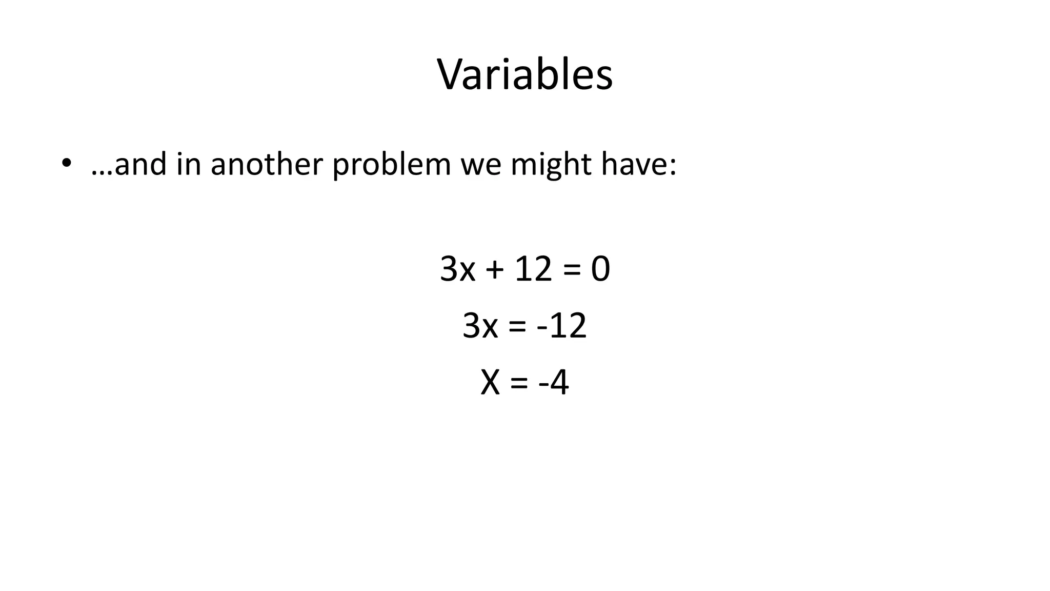
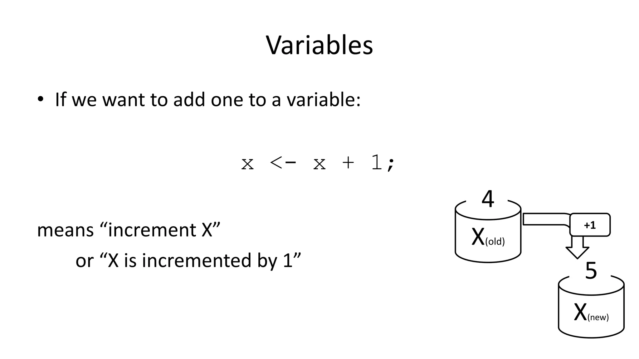
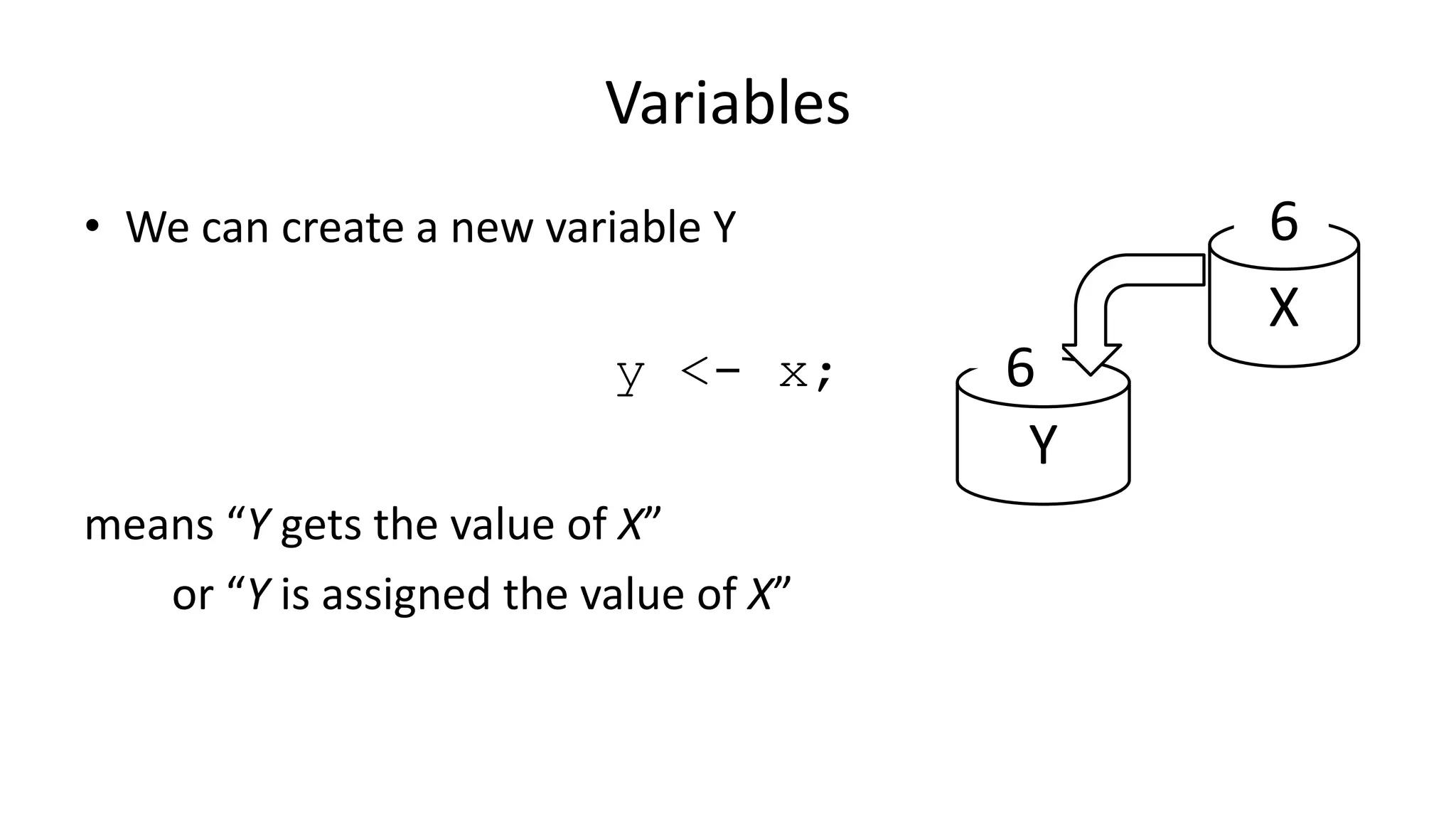
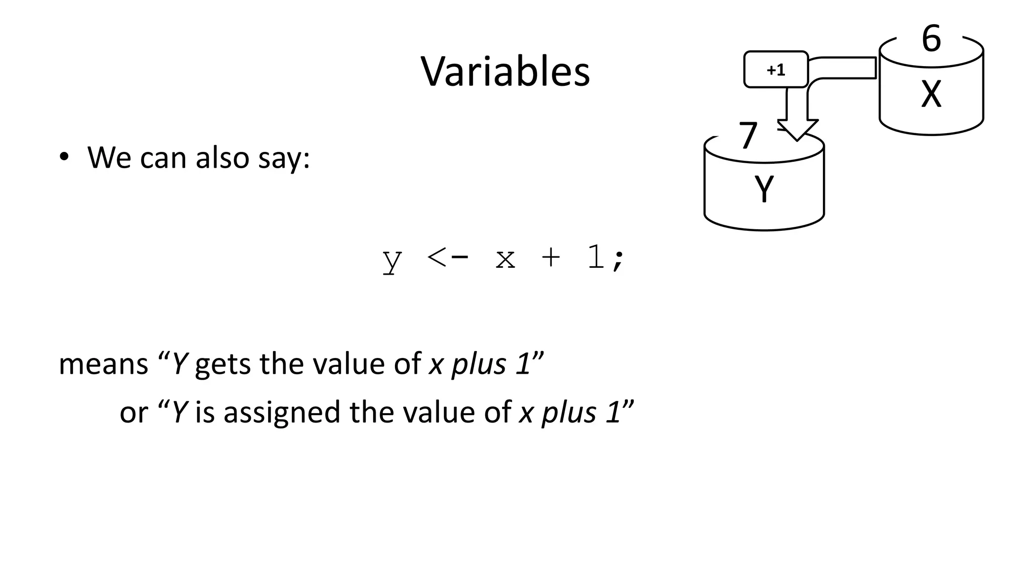
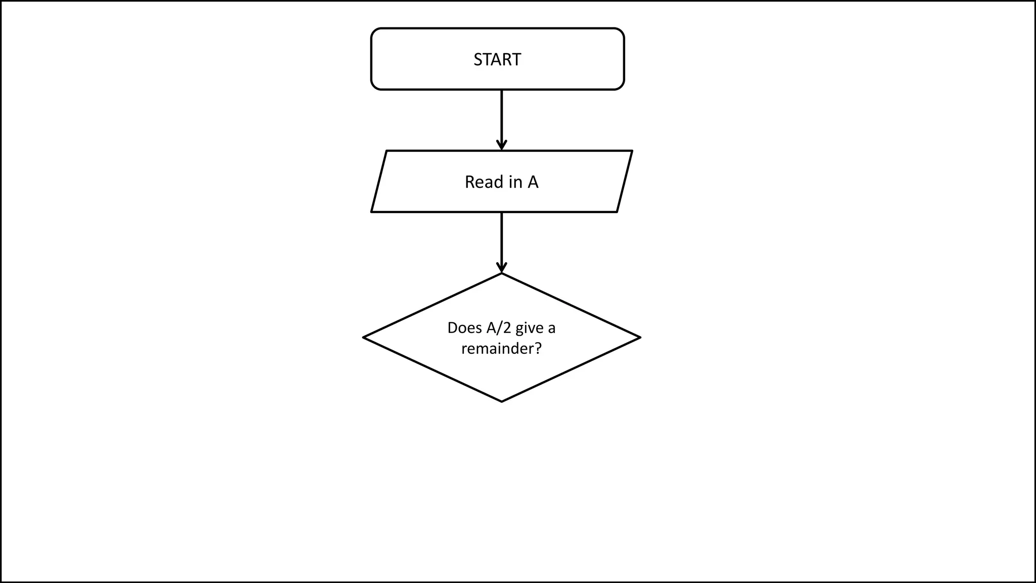
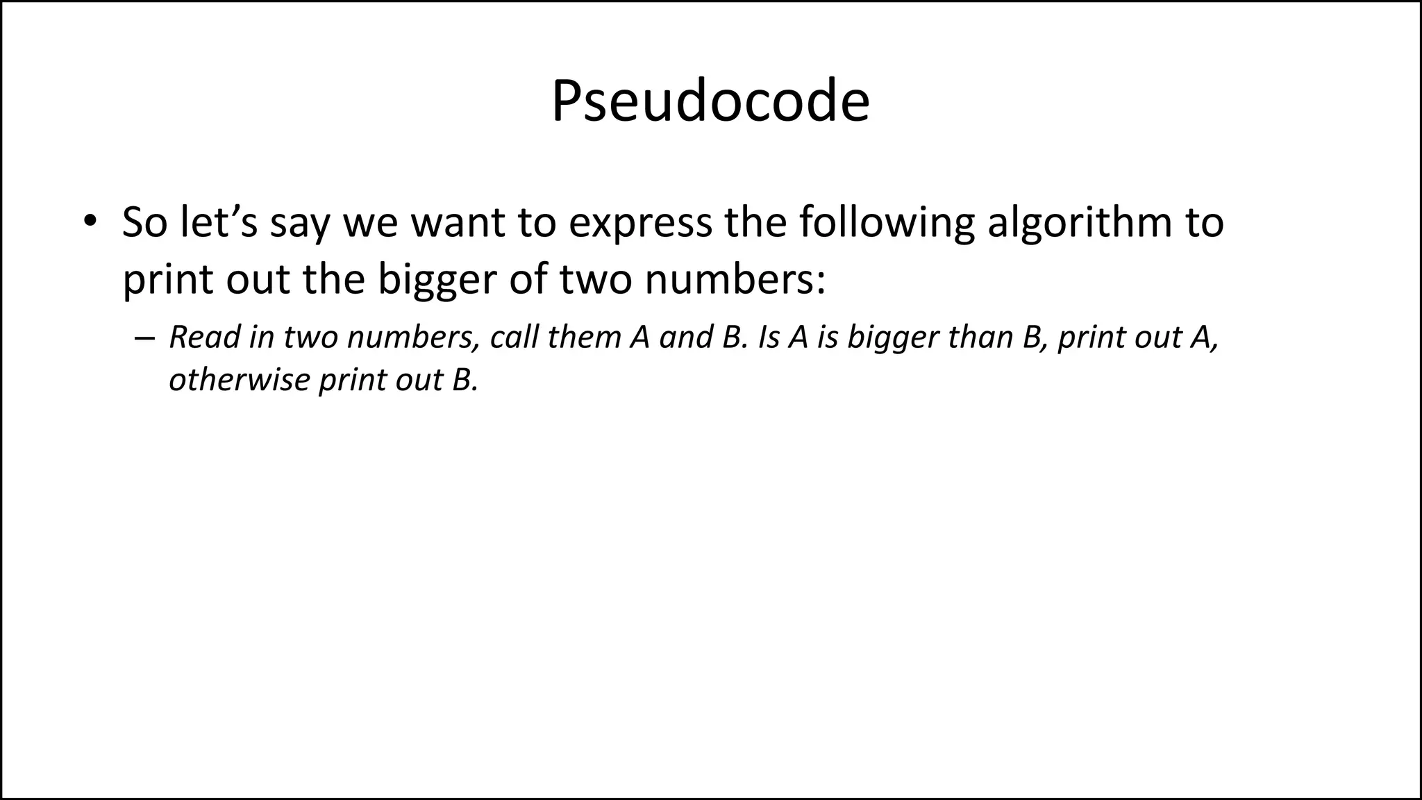
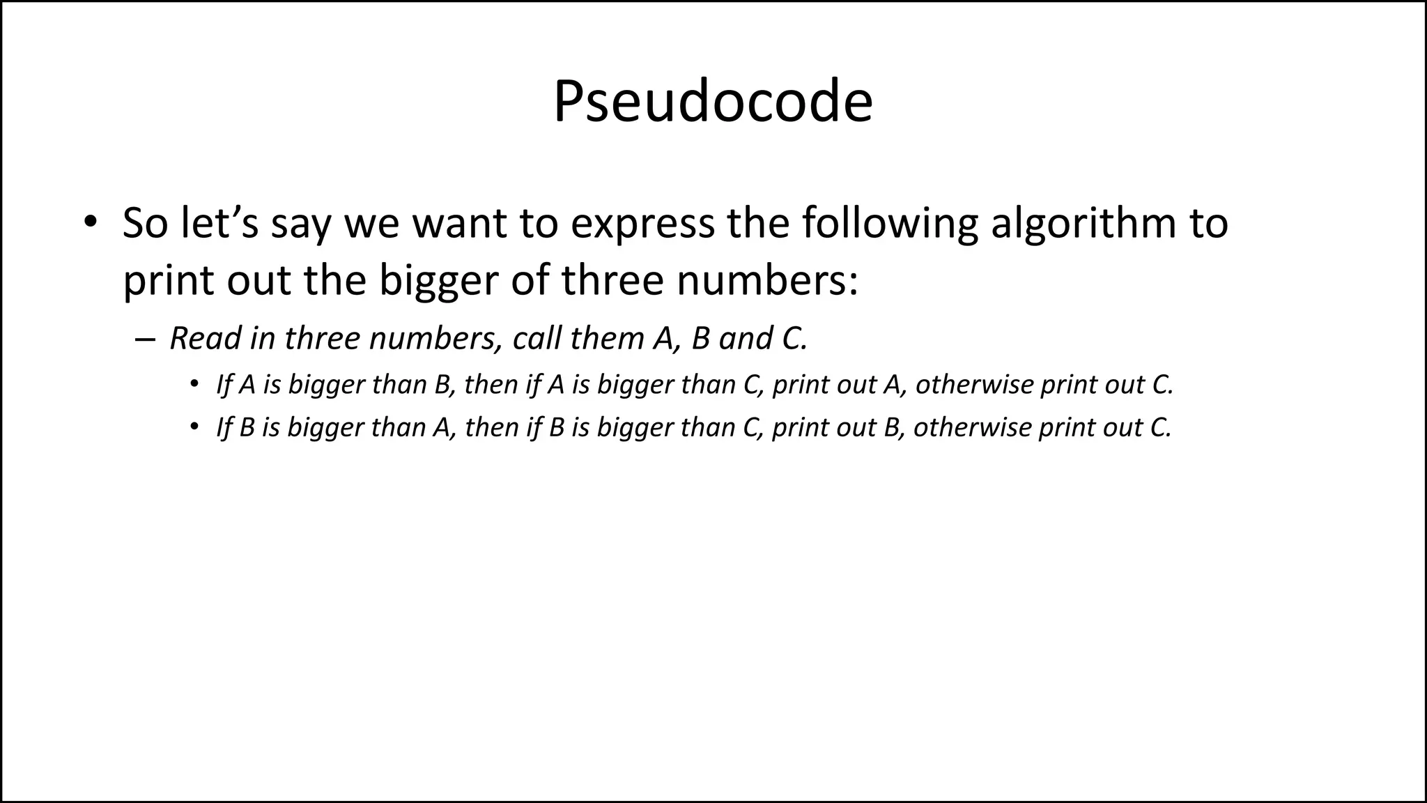
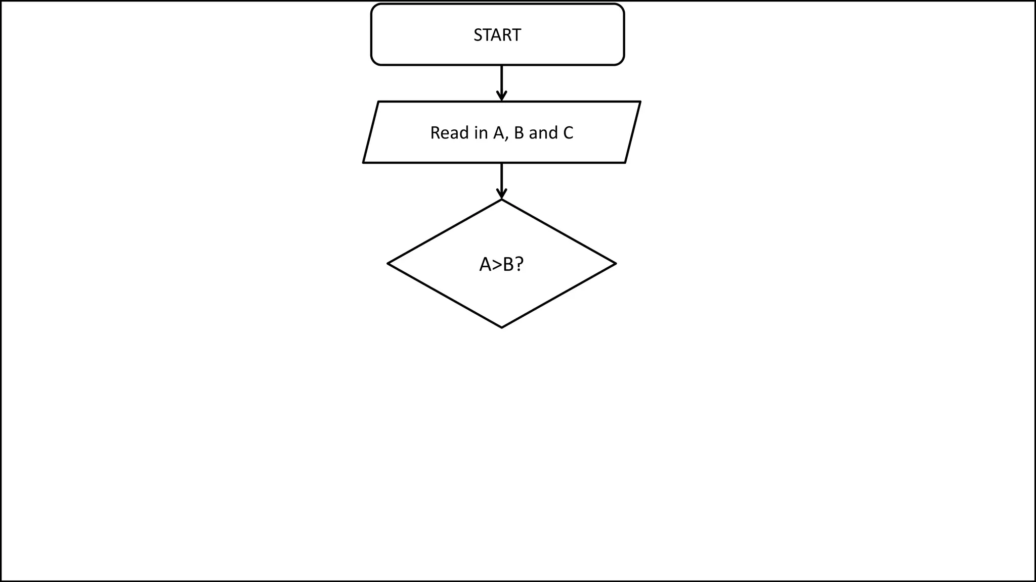
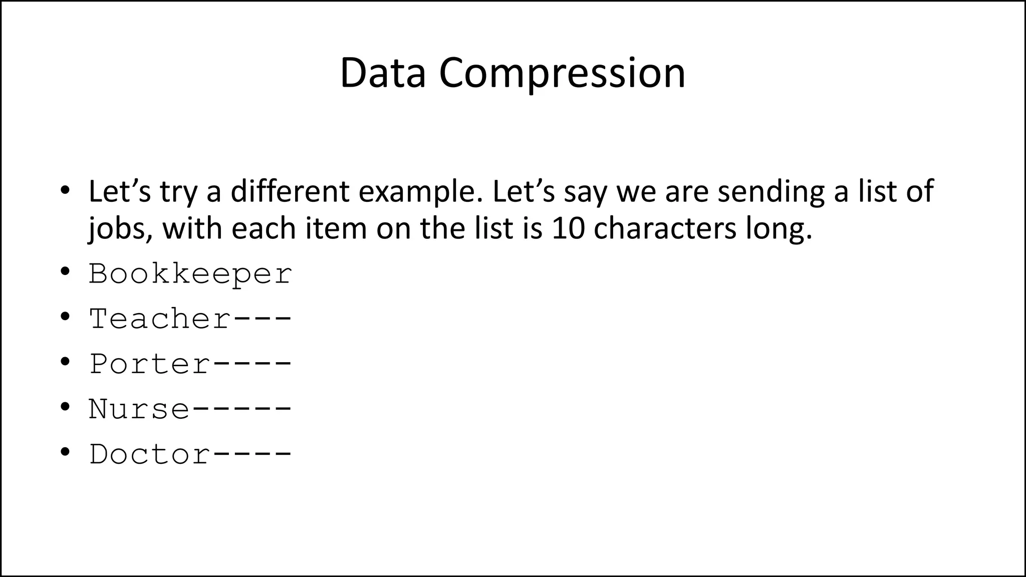
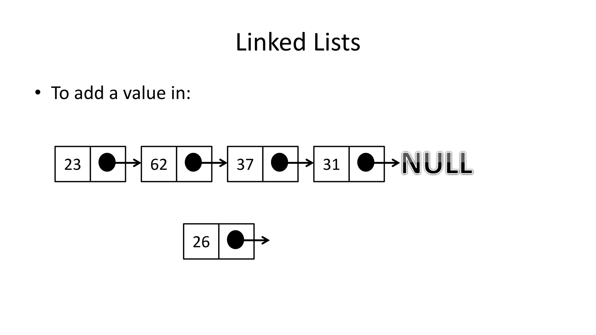
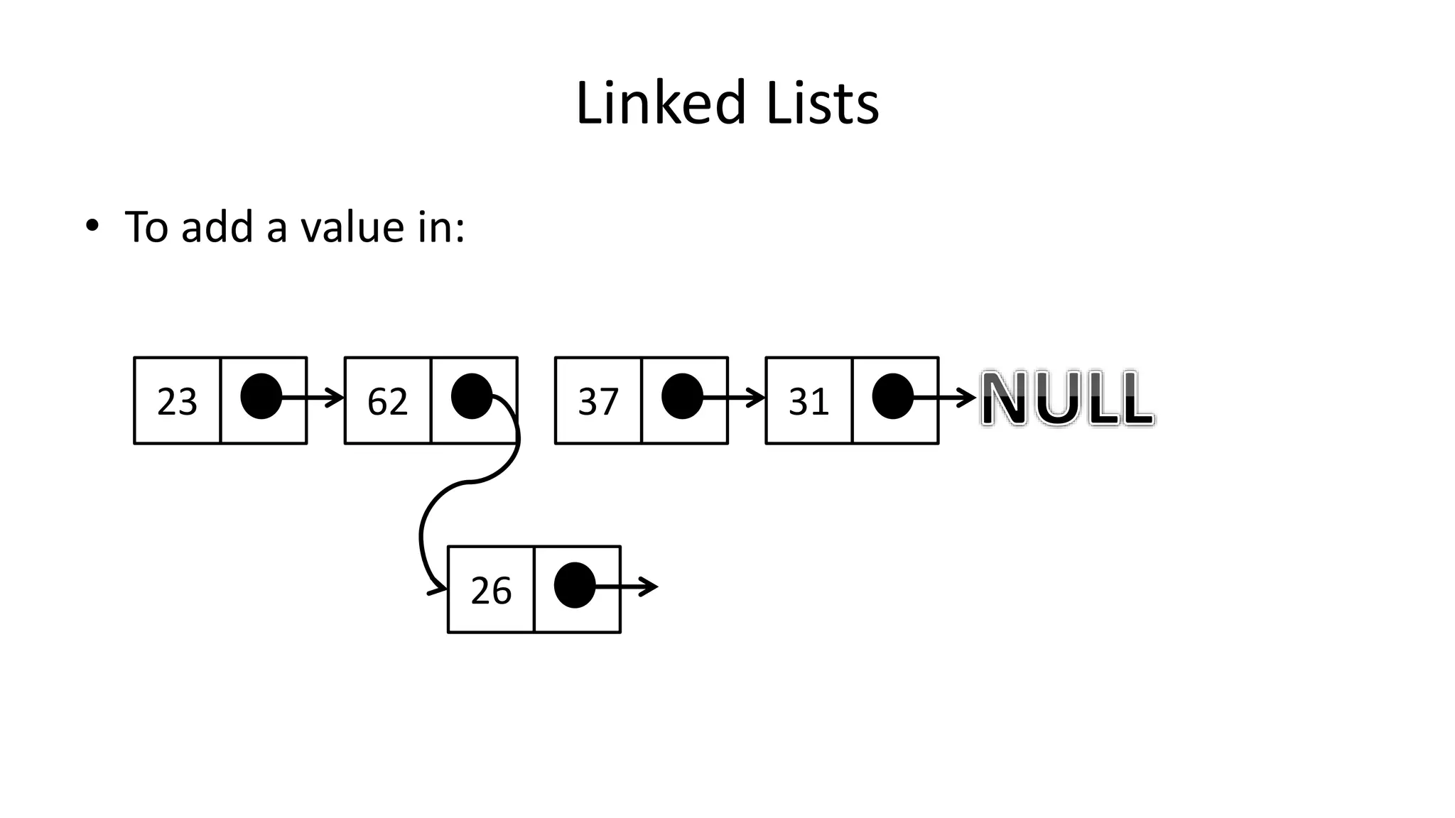
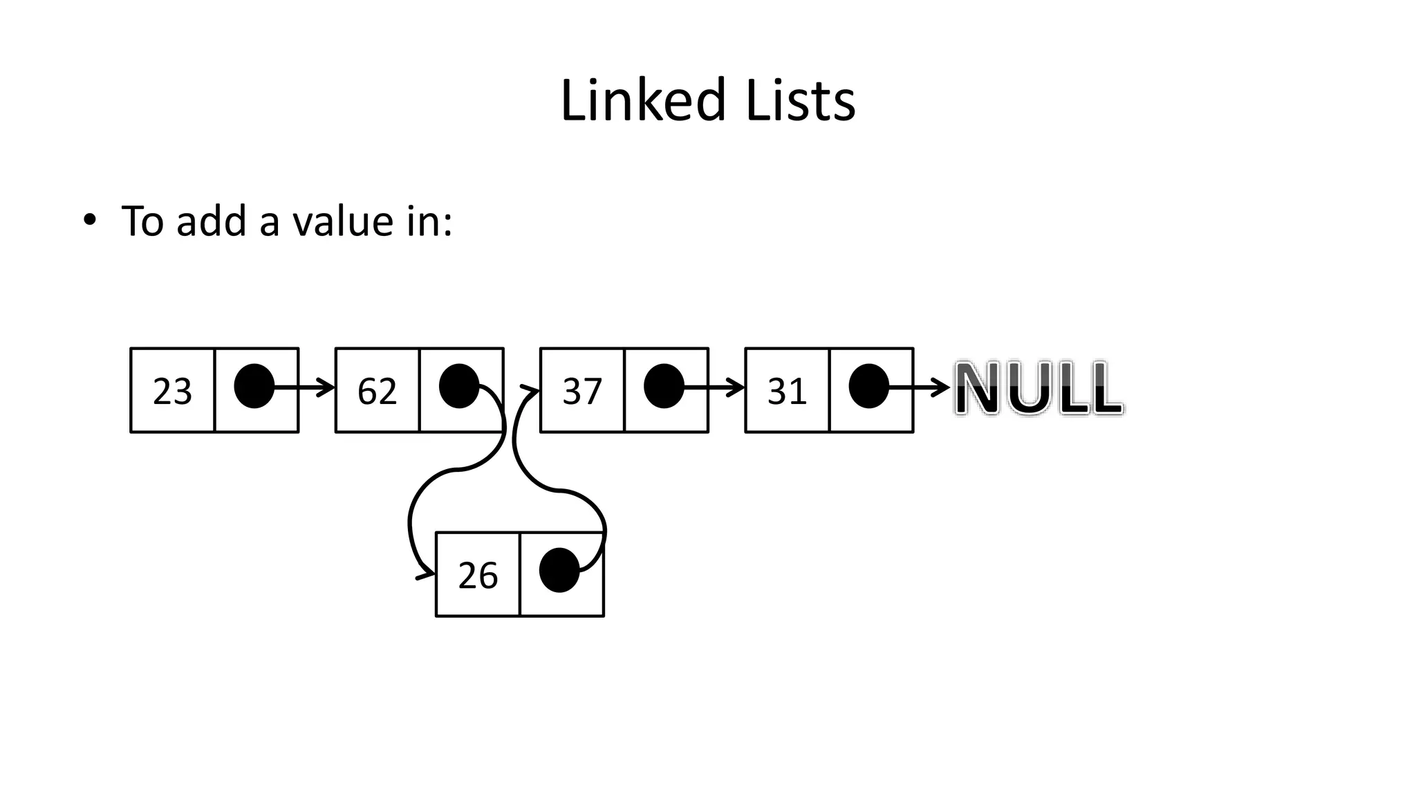
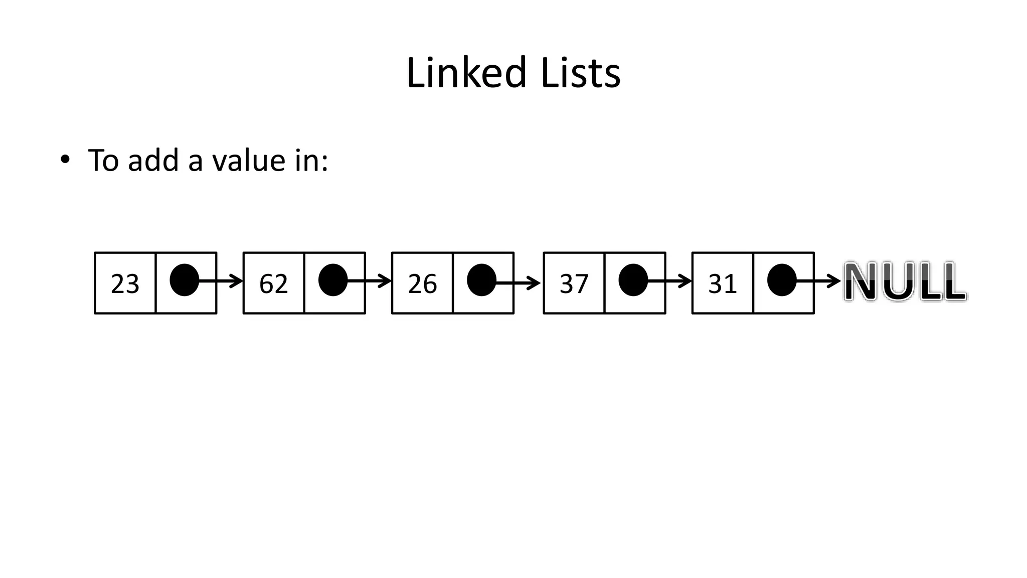
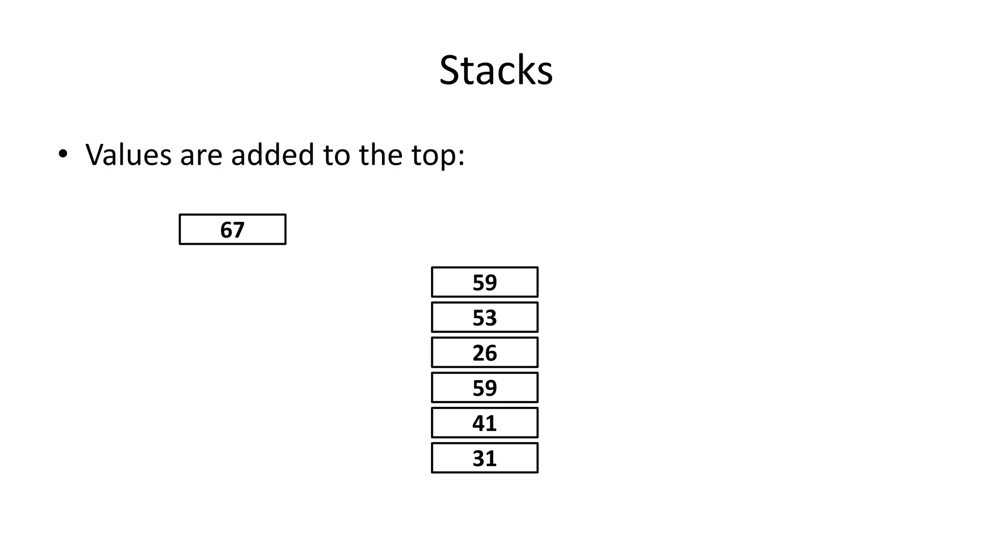
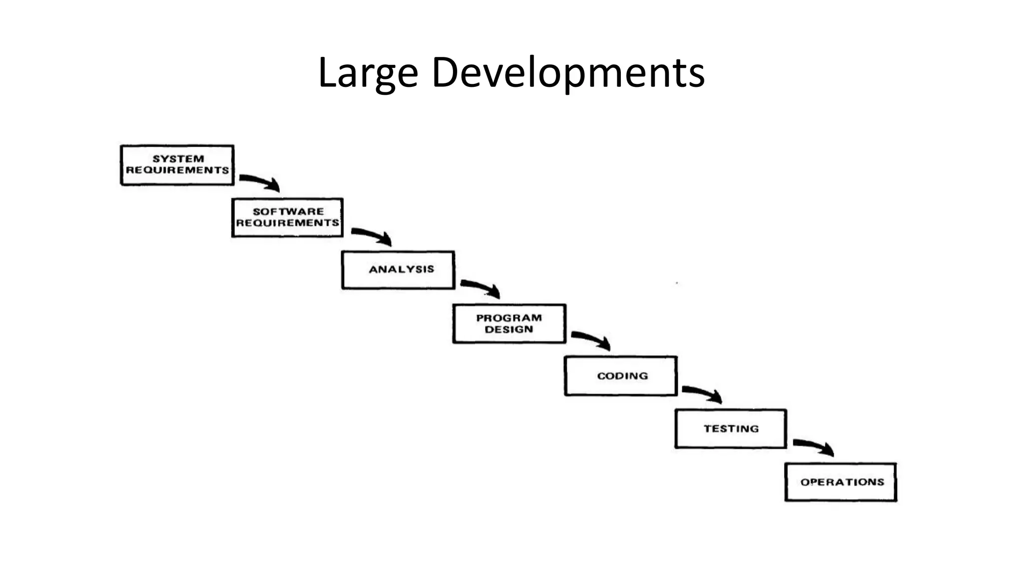
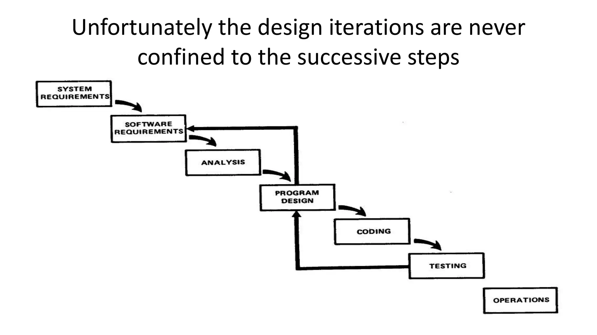
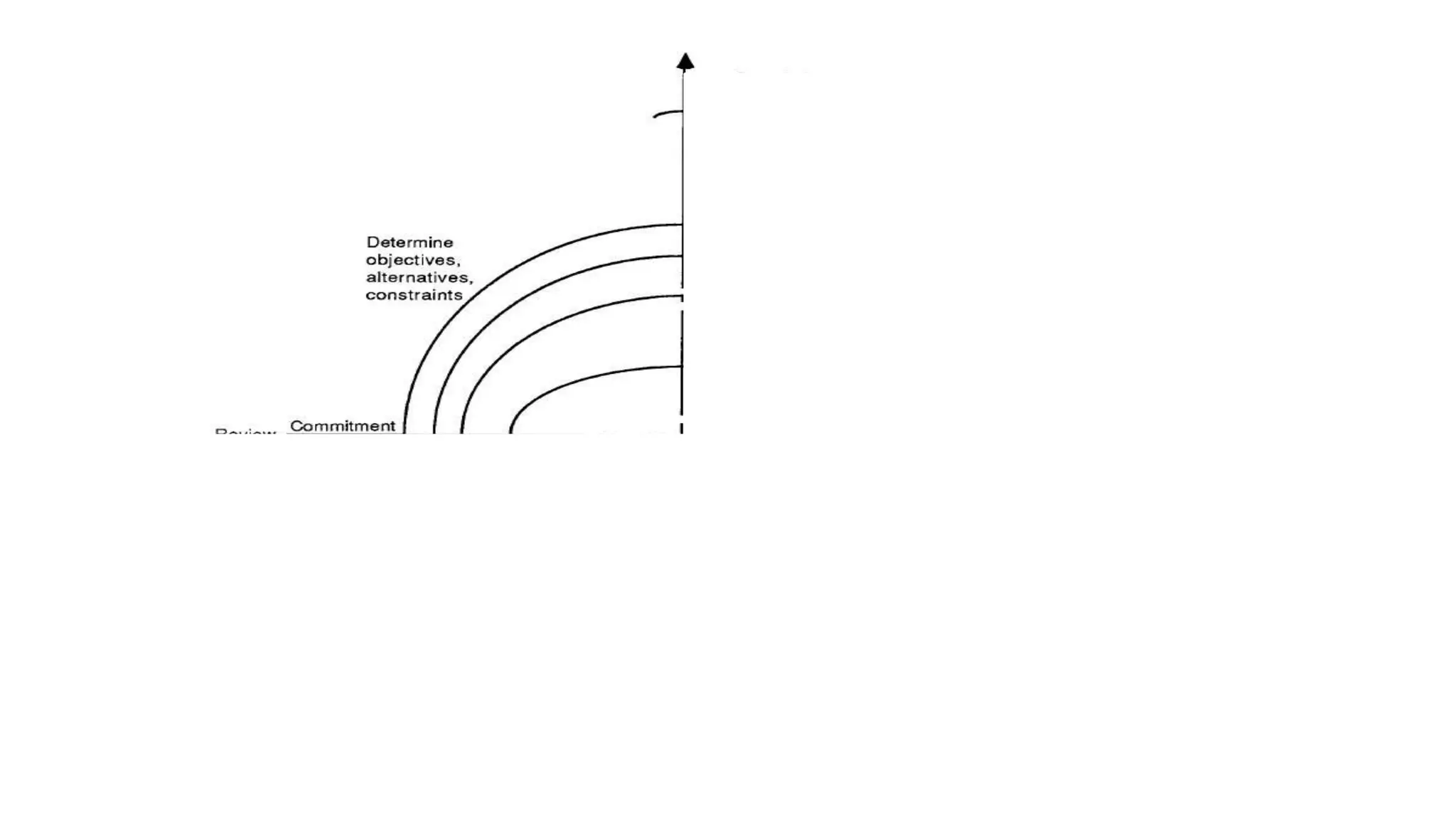
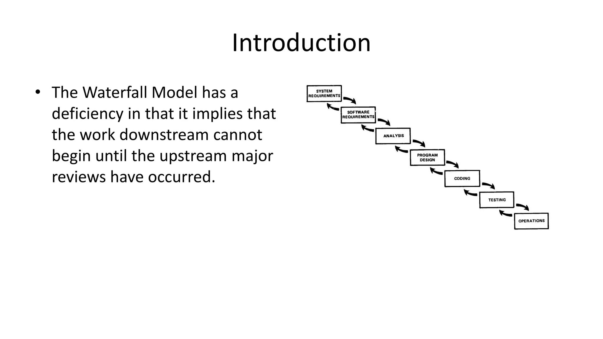
This document provides an overview of a complete program design course that teaches programming, program design, and algorithms using pseudocode. The course assumes no prior knowledge and aims to teach fundamental programming concepts like procedural programming, good program design practices, and elementary algorithms and data structures. The learning outcomes include being able to design and write basic programs in a structured procedural language, use development tools to compile and run code, divide programs into modules, test programs, and implement basic algorithms and data structures. The indicative syllabus covers topics like basic data types, input/output, programming structures like conditionals and loops, functions, arrays, sorting algorithms, testing, debugging, and documentation. Assessment includes a written exam and continuous assessment.


![Algorithm Design and Problem Solving [Autosaved].pptx](https://cdn.slidesharecdn.com/ss_thumbnails/algorithmdesignandproblemsolvingautosaved-230525024624-6a6fb3b2-thumbnail.jpg?width=640&height=640&fit=bounds)


![SHS_Core_CAE_Q3_LE1 FOR THIRD [FINAL].pdf](https://cdn.slidesharecdn.com/ss_thumbnails/shscorecaeq3le1final-251116055110-e3081055-thumbnail.jpg?width=640&height=640&fit=bounds)


