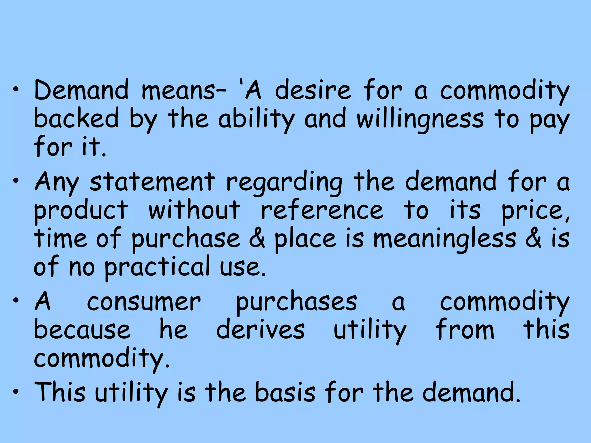
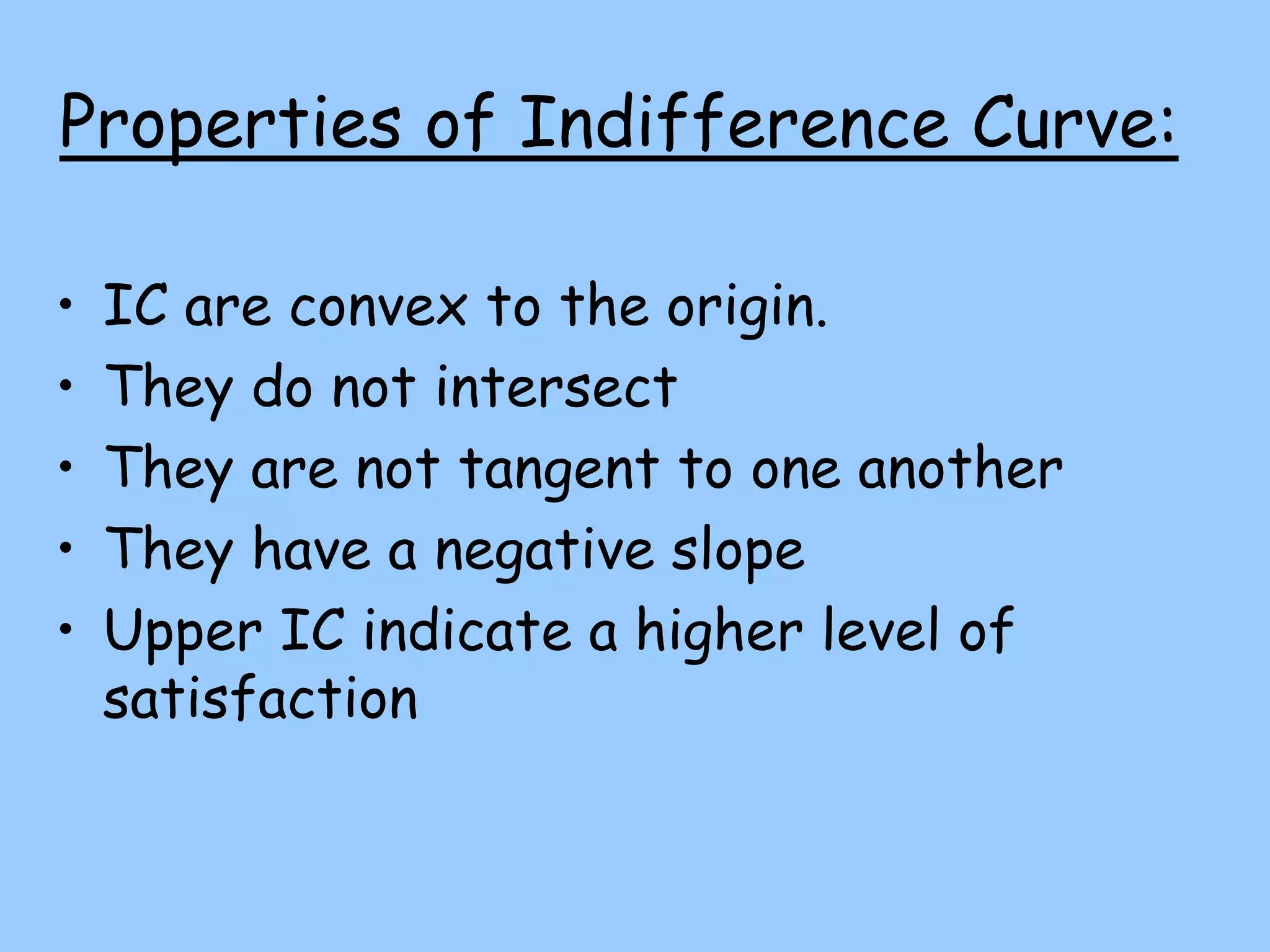
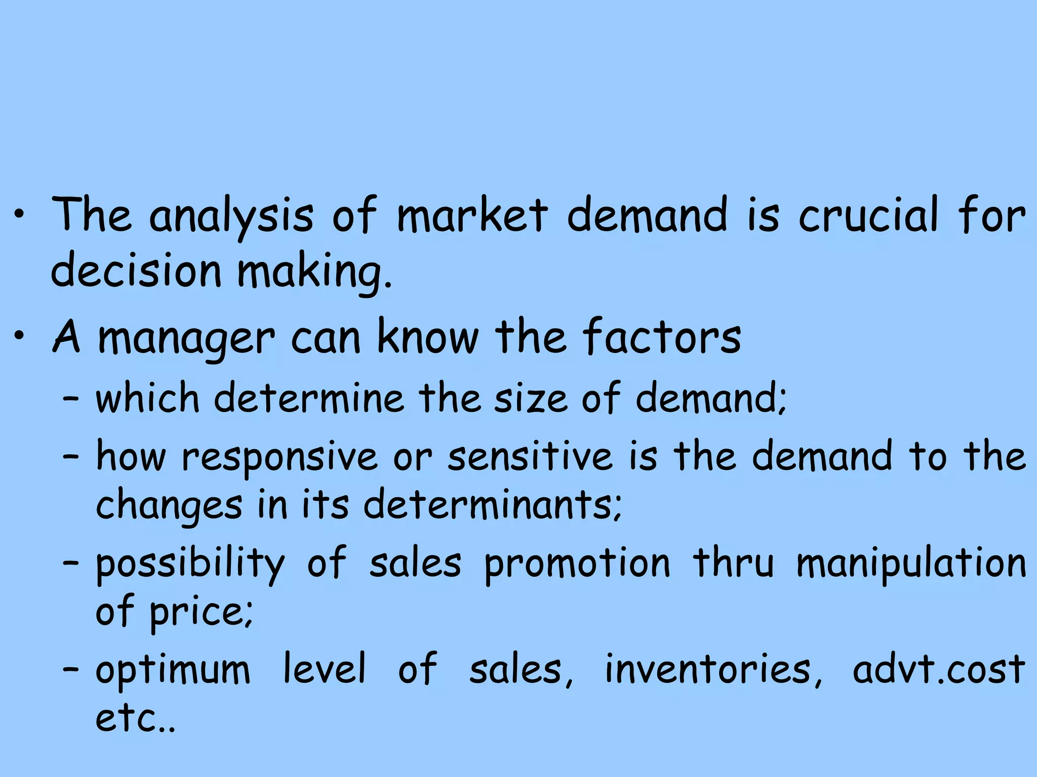
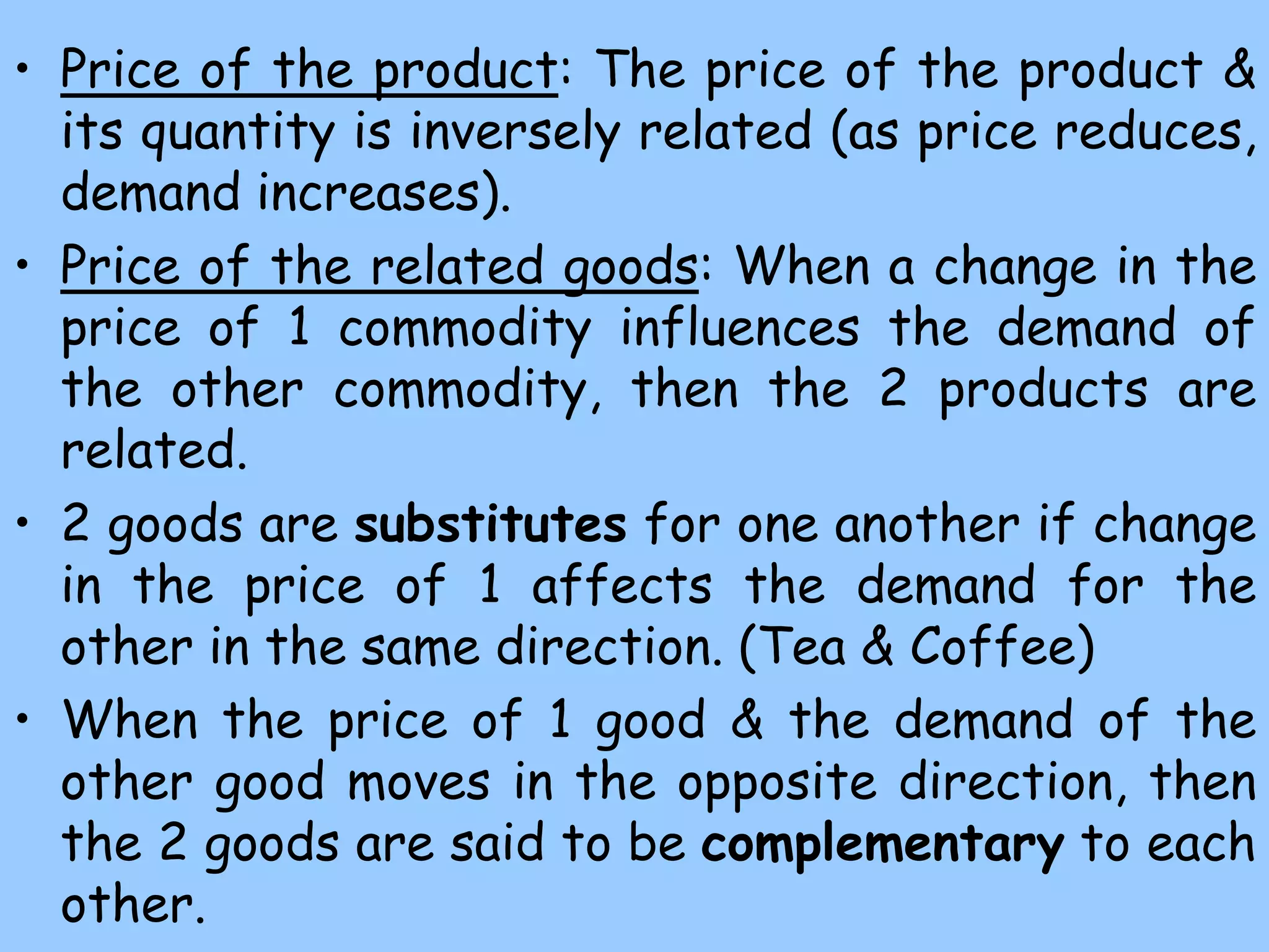
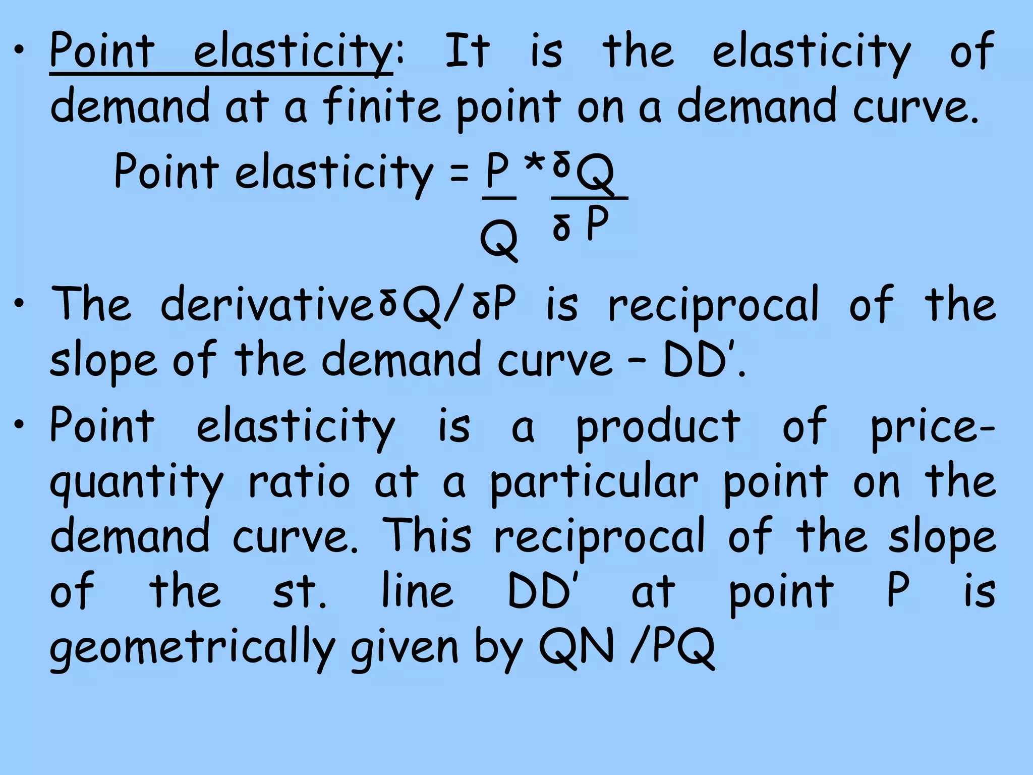
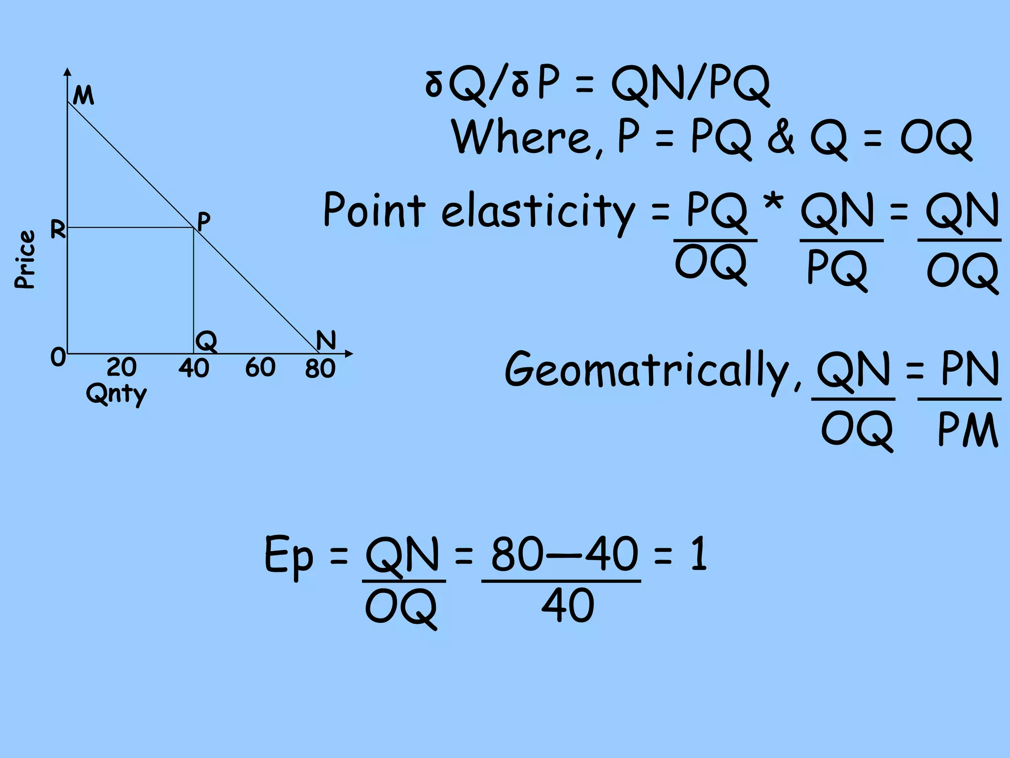
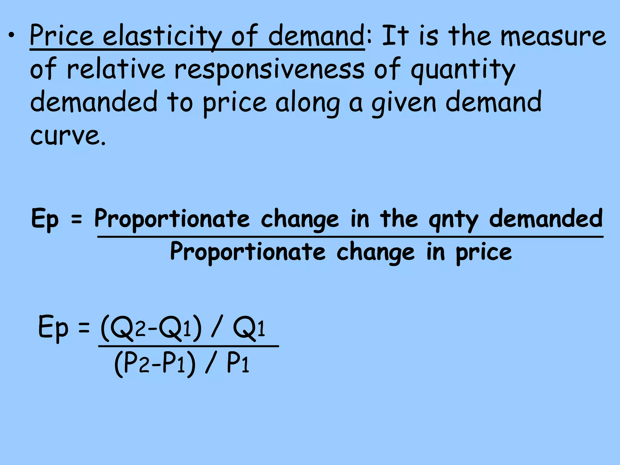
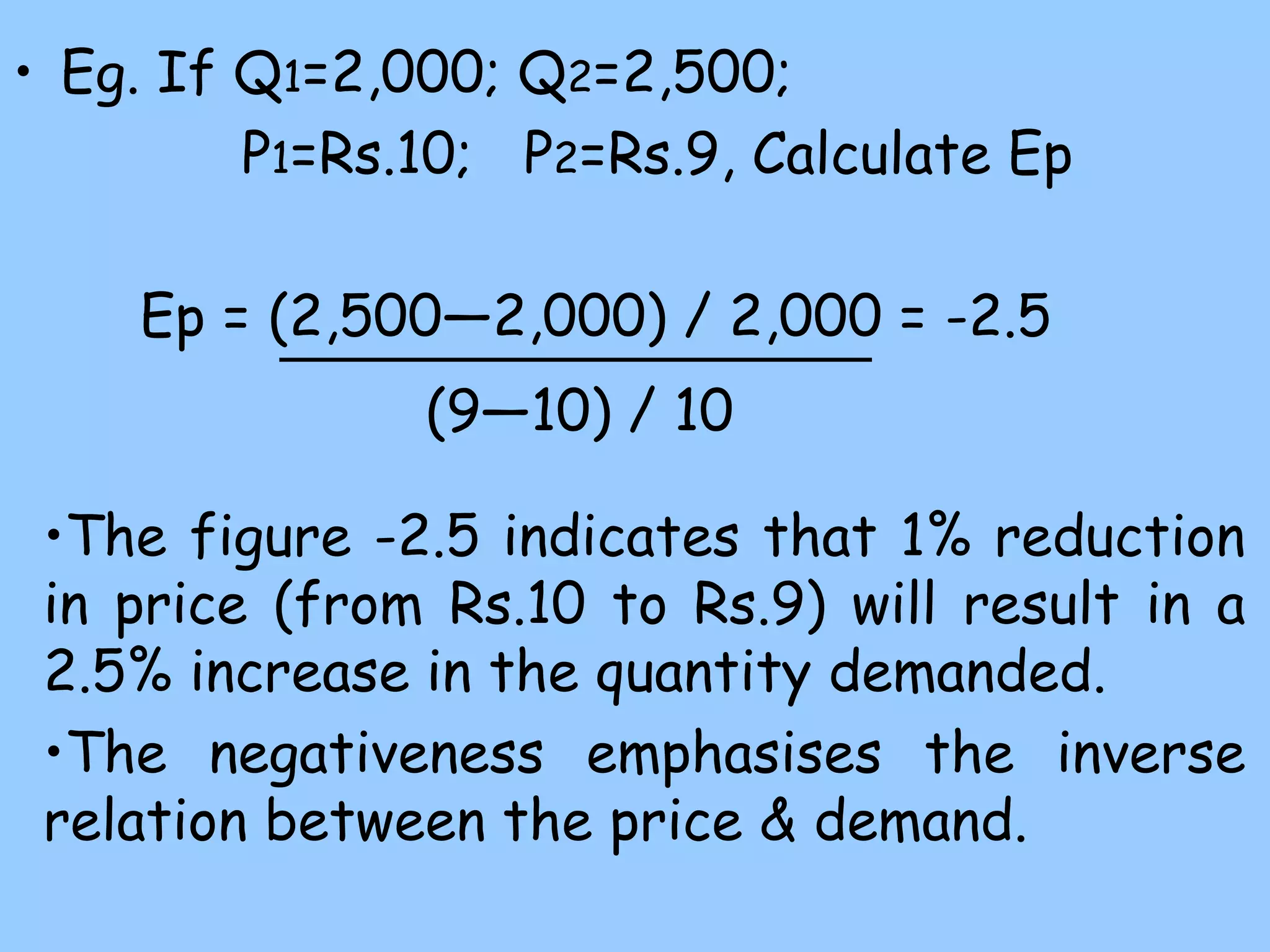
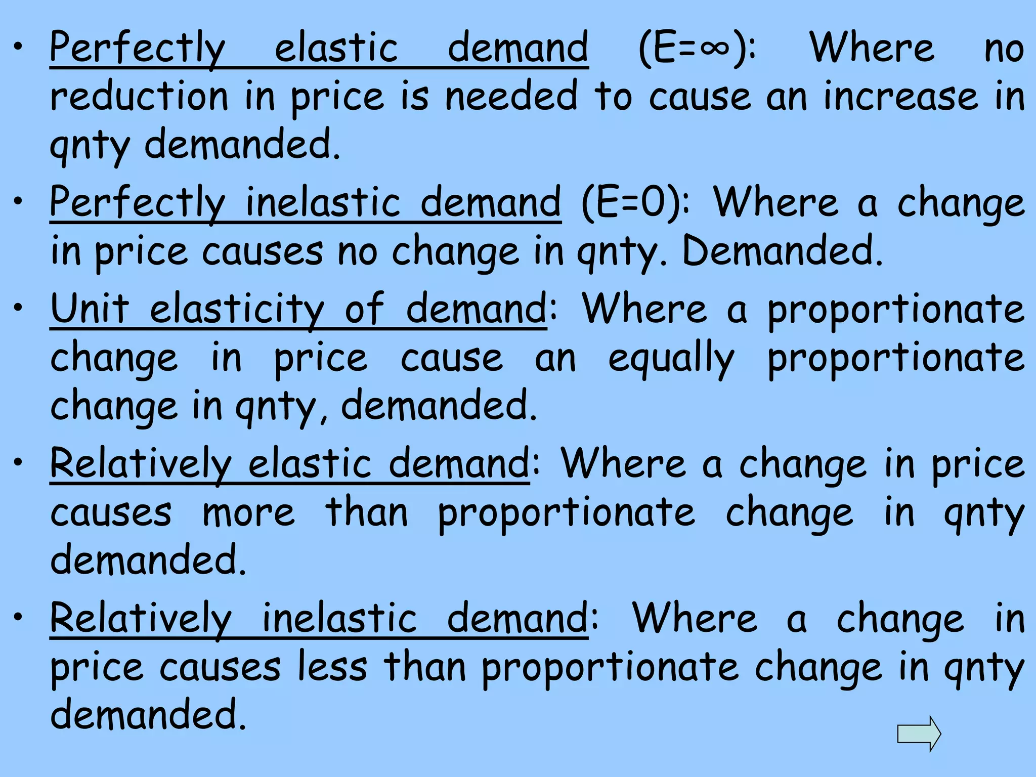
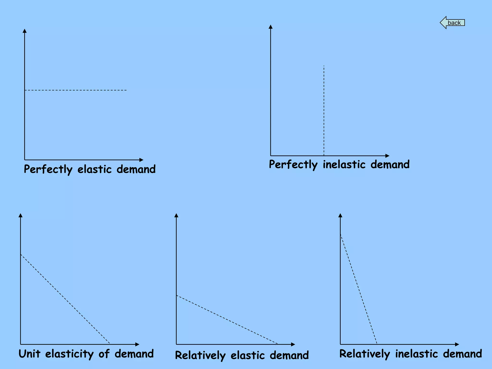
1) Demand analysis examines how consumer demand for a product is determined based on factors like price, income, tastes, and prices of substitutes and complements. Consumer demand at the individual and market level can be modeled using demand functions.
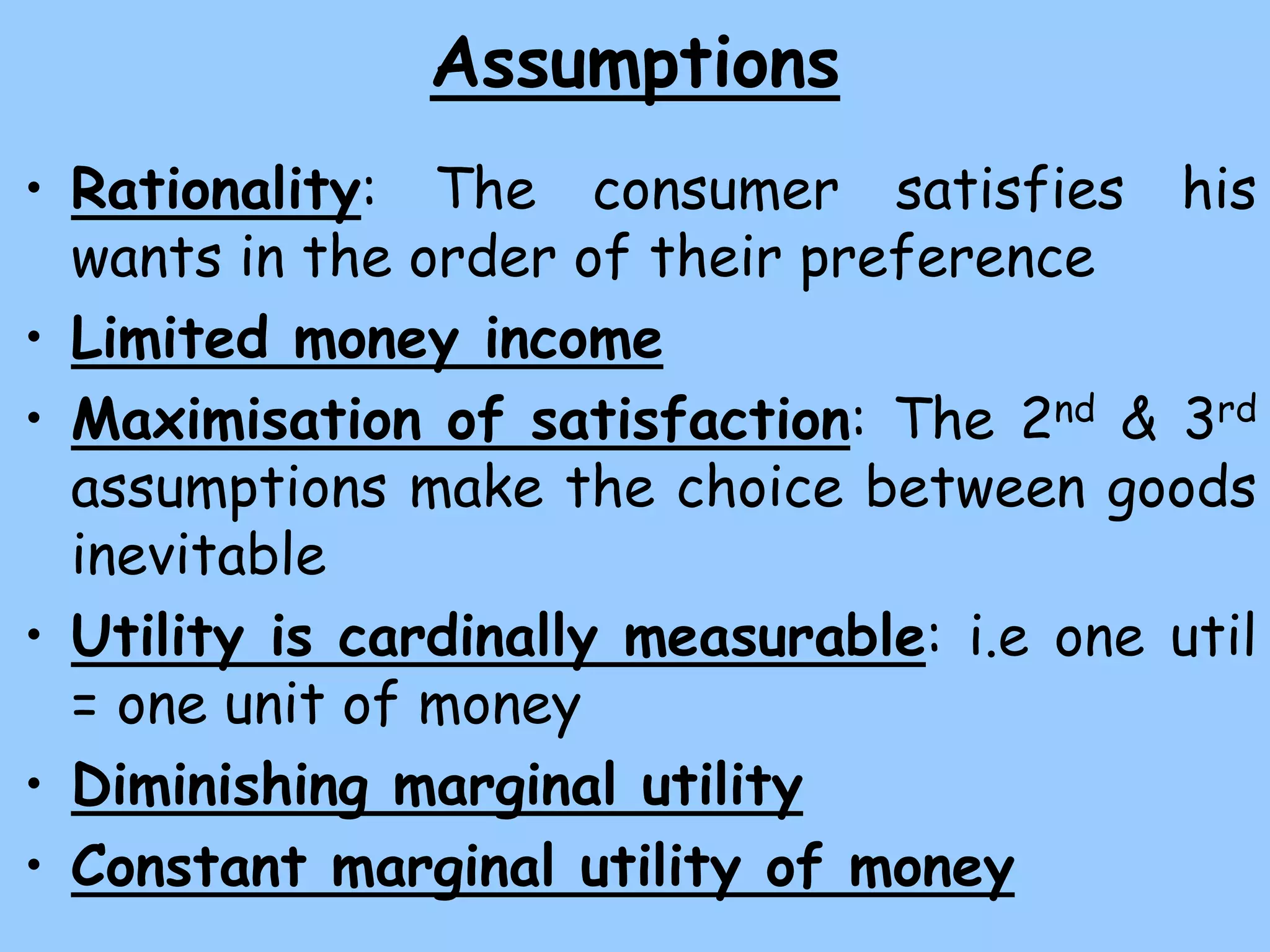
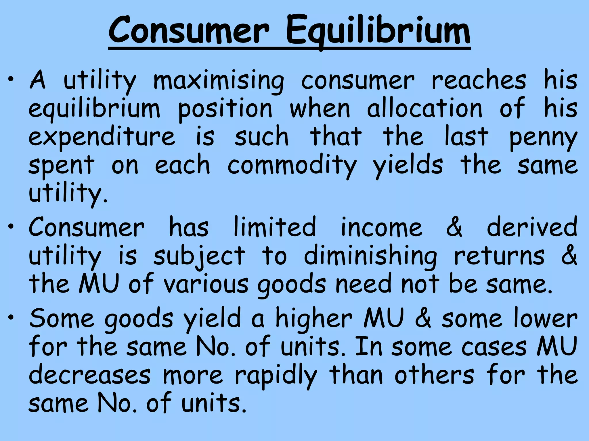
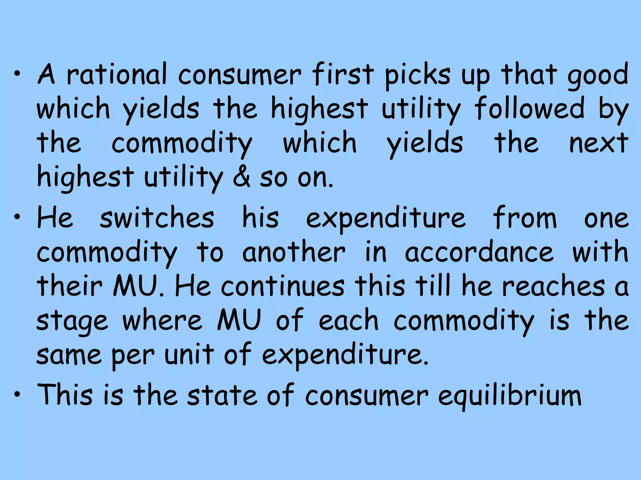
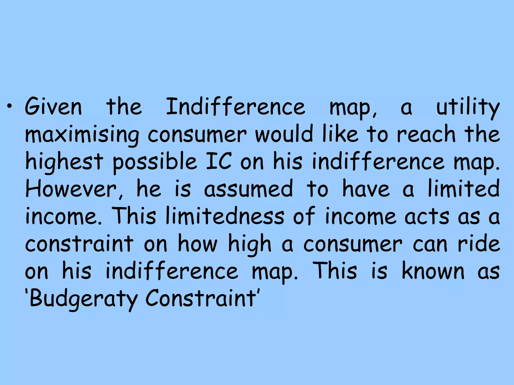
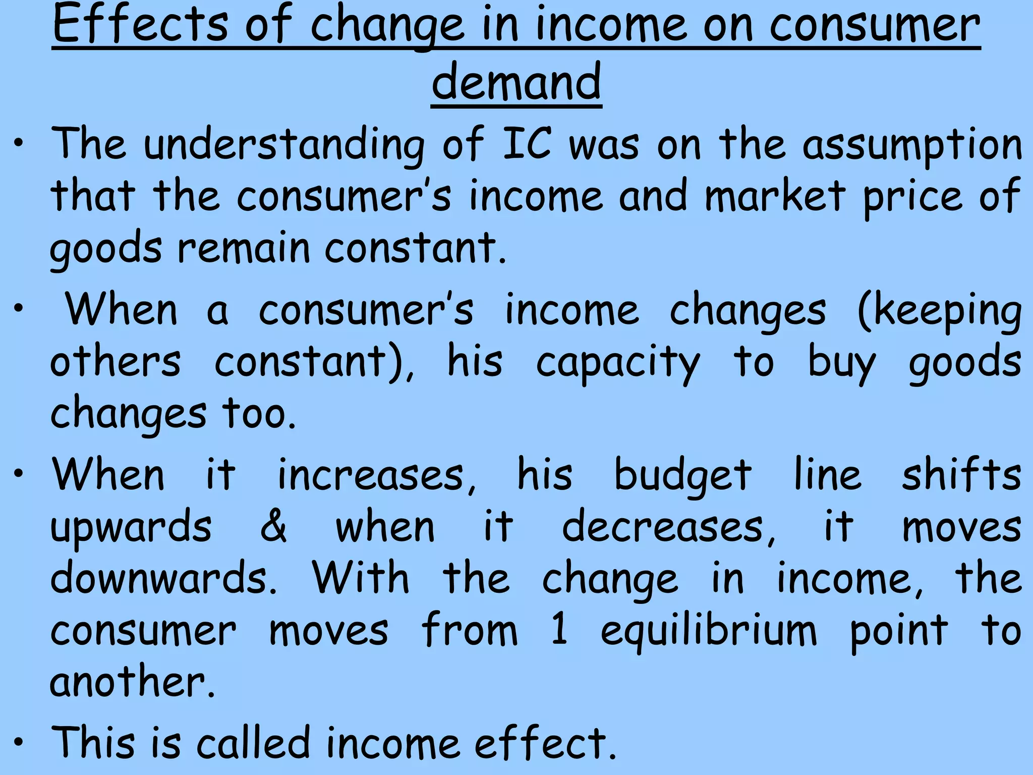
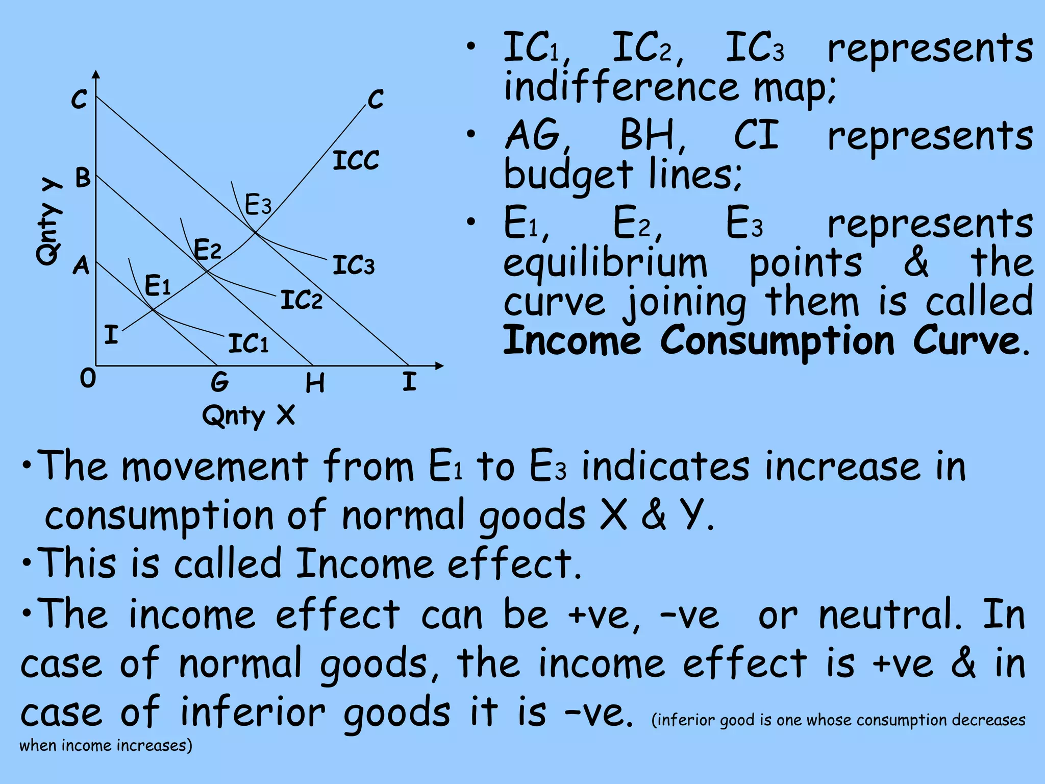
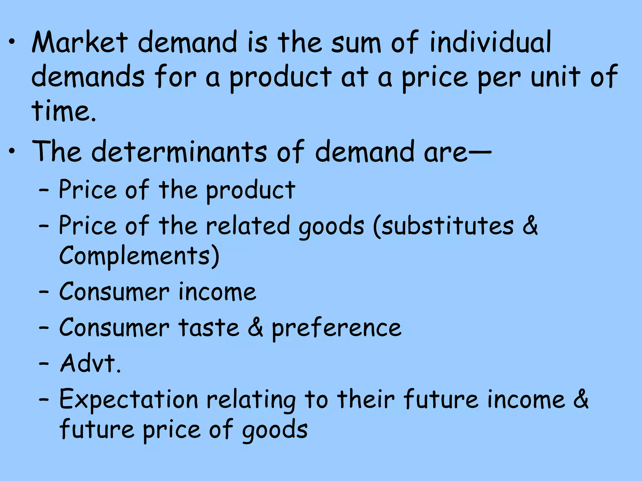
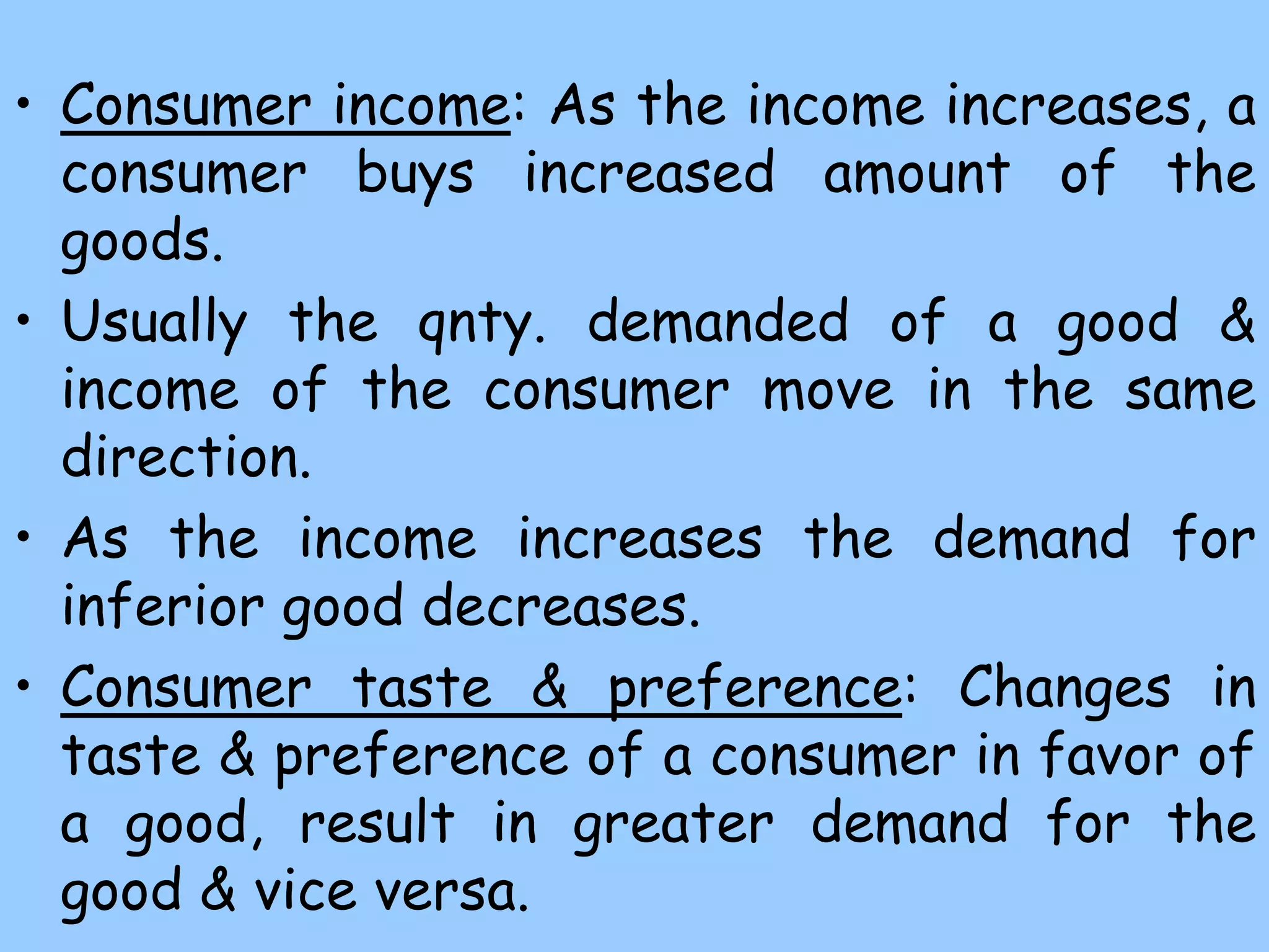
2) At the individual level, consumers aim to maximize utility subject to a budget constraint. They allocate spending across goods until the marginal utility per rupee is equal for all goods. At the market level, demand is the sum of individual demands and is influenced by price, income, population, and other factors.
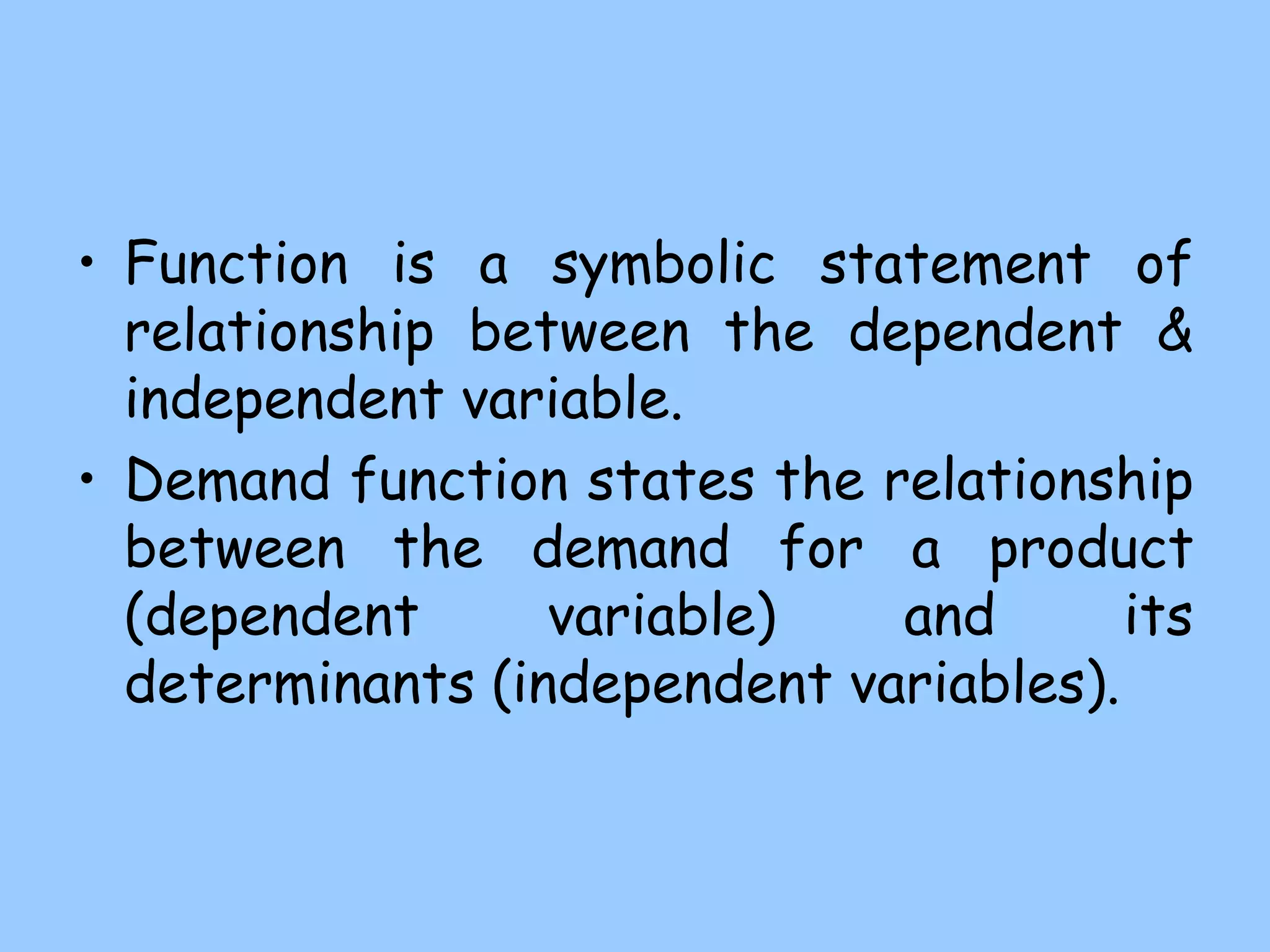
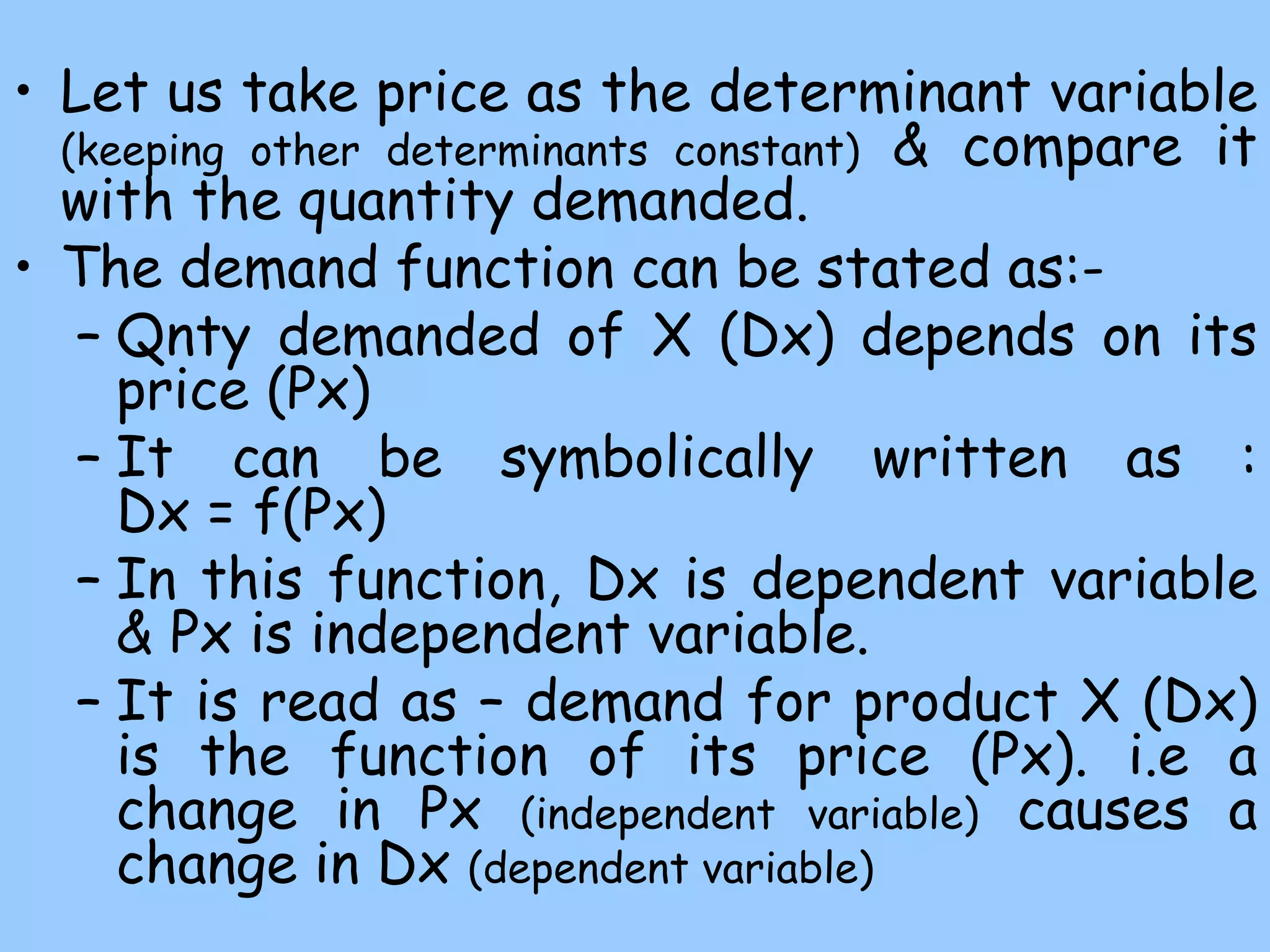
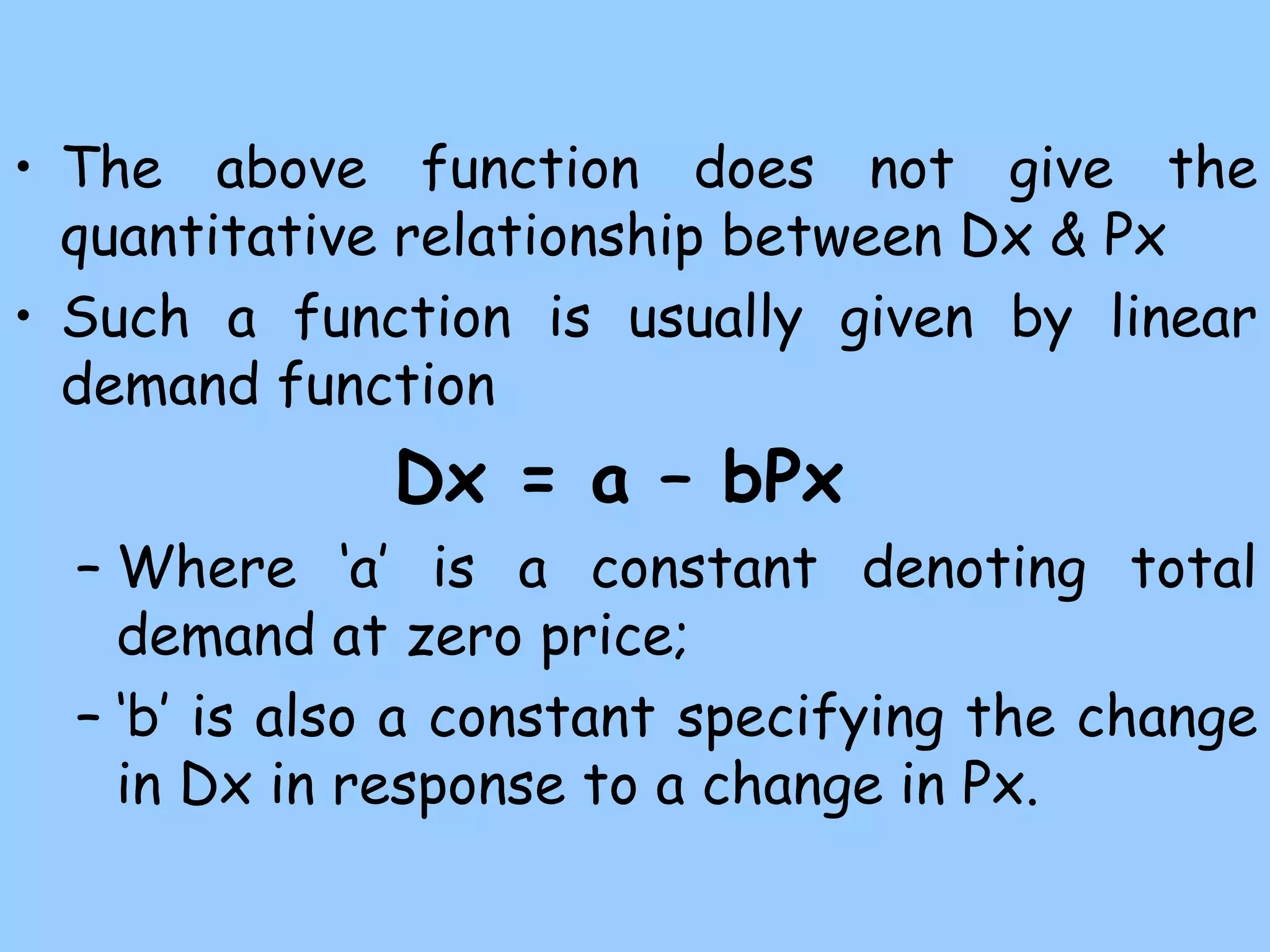
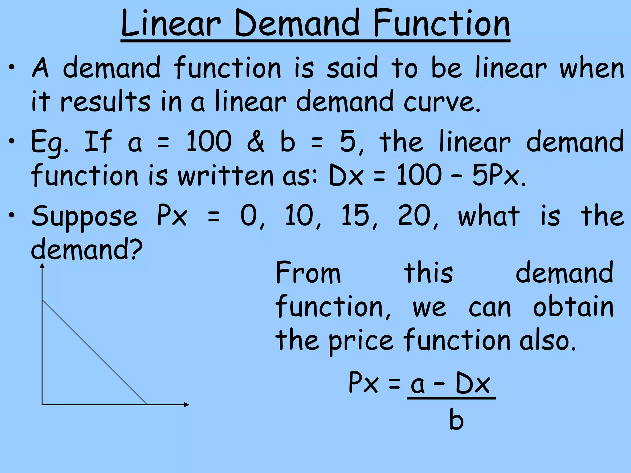
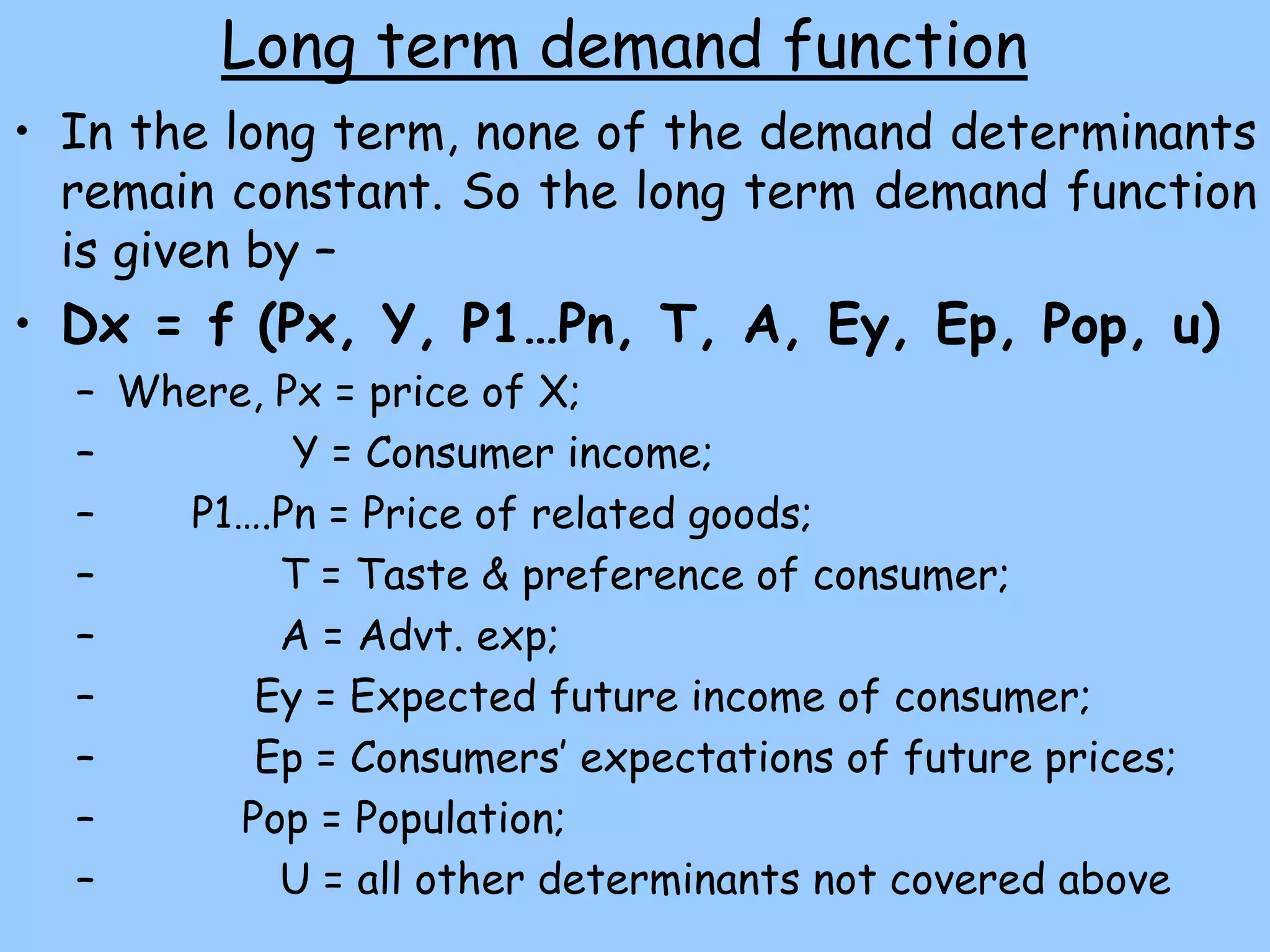
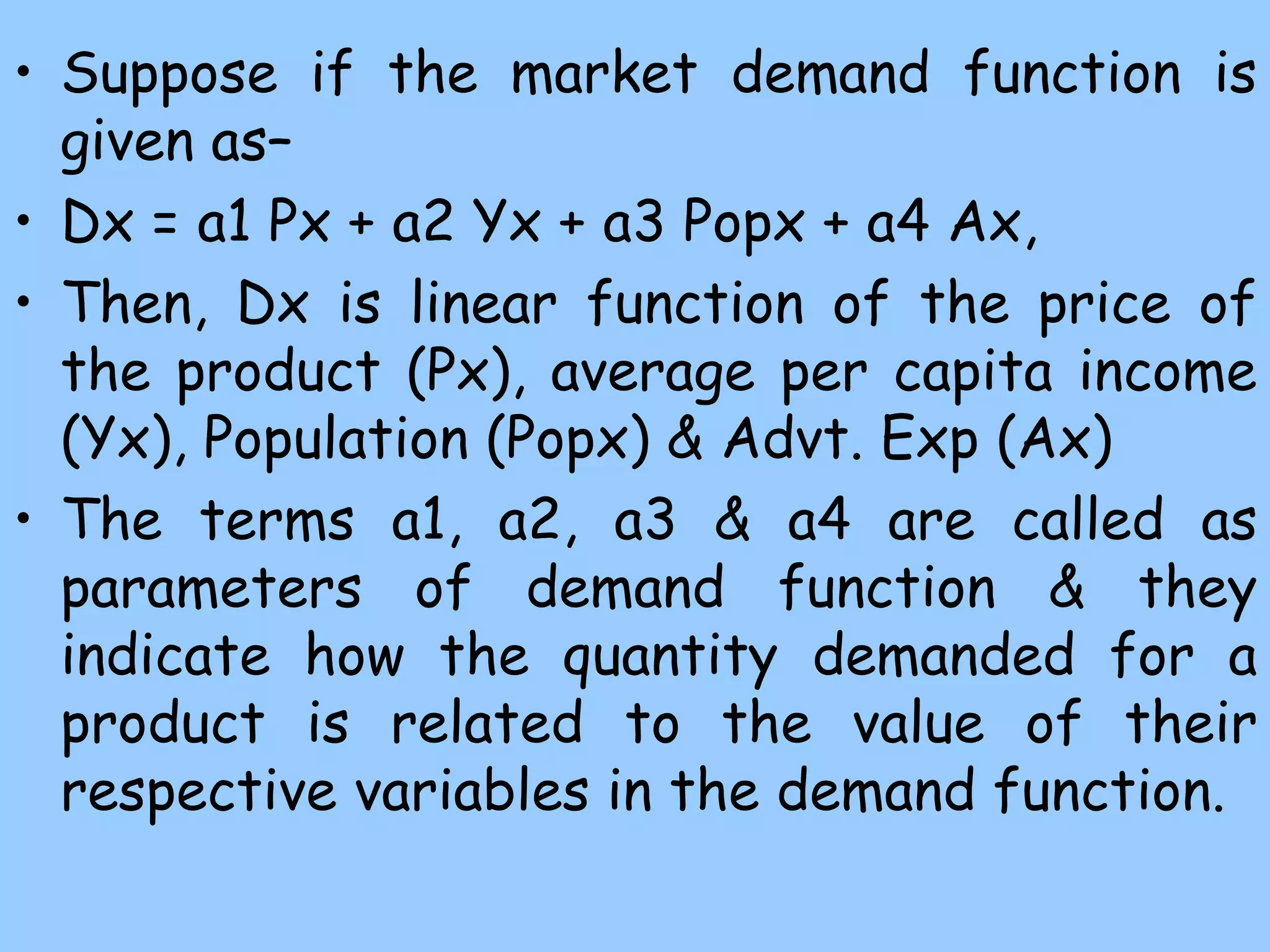
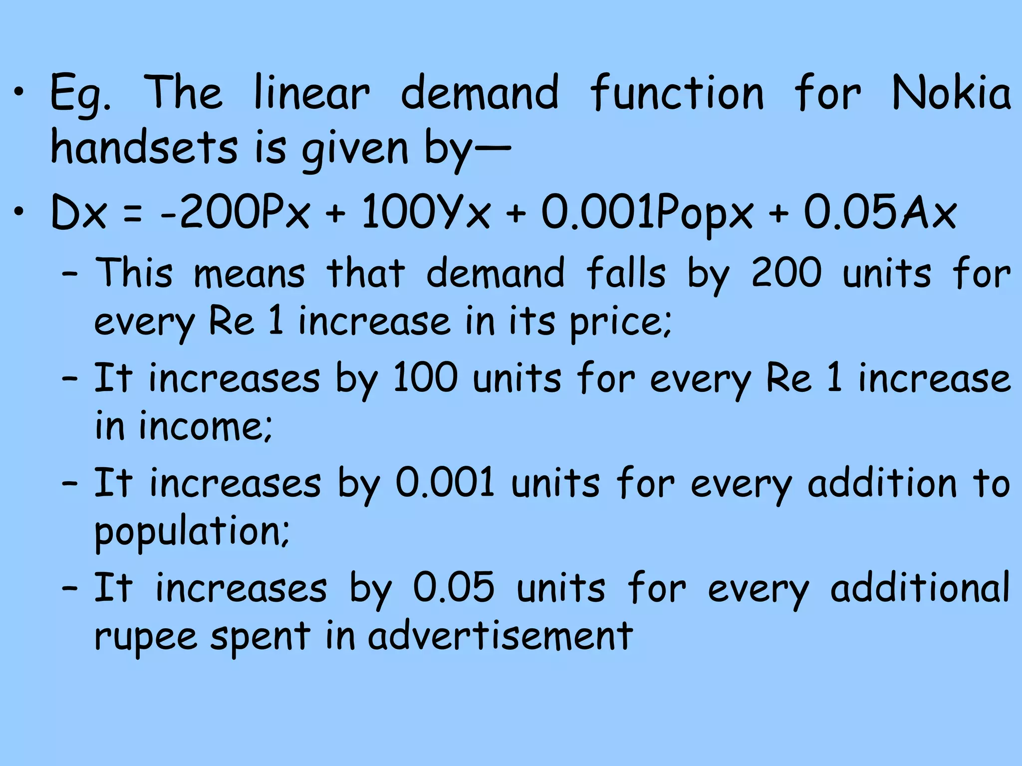
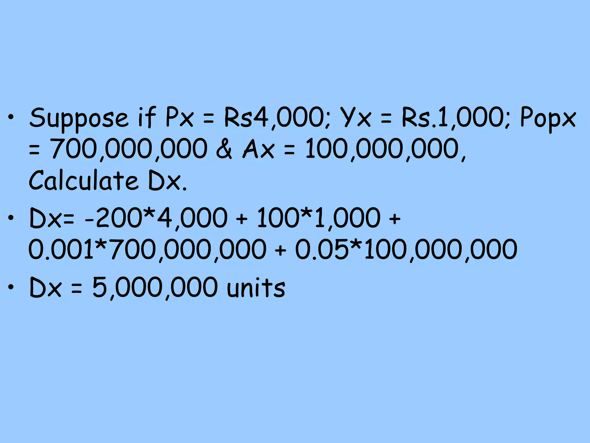
3) Demand functions express the quantitative relationship between demand for a product and its determinants. They can be linear or nonlinear. The slope of the linear demand