Download as PDF, PPTX

![Schema
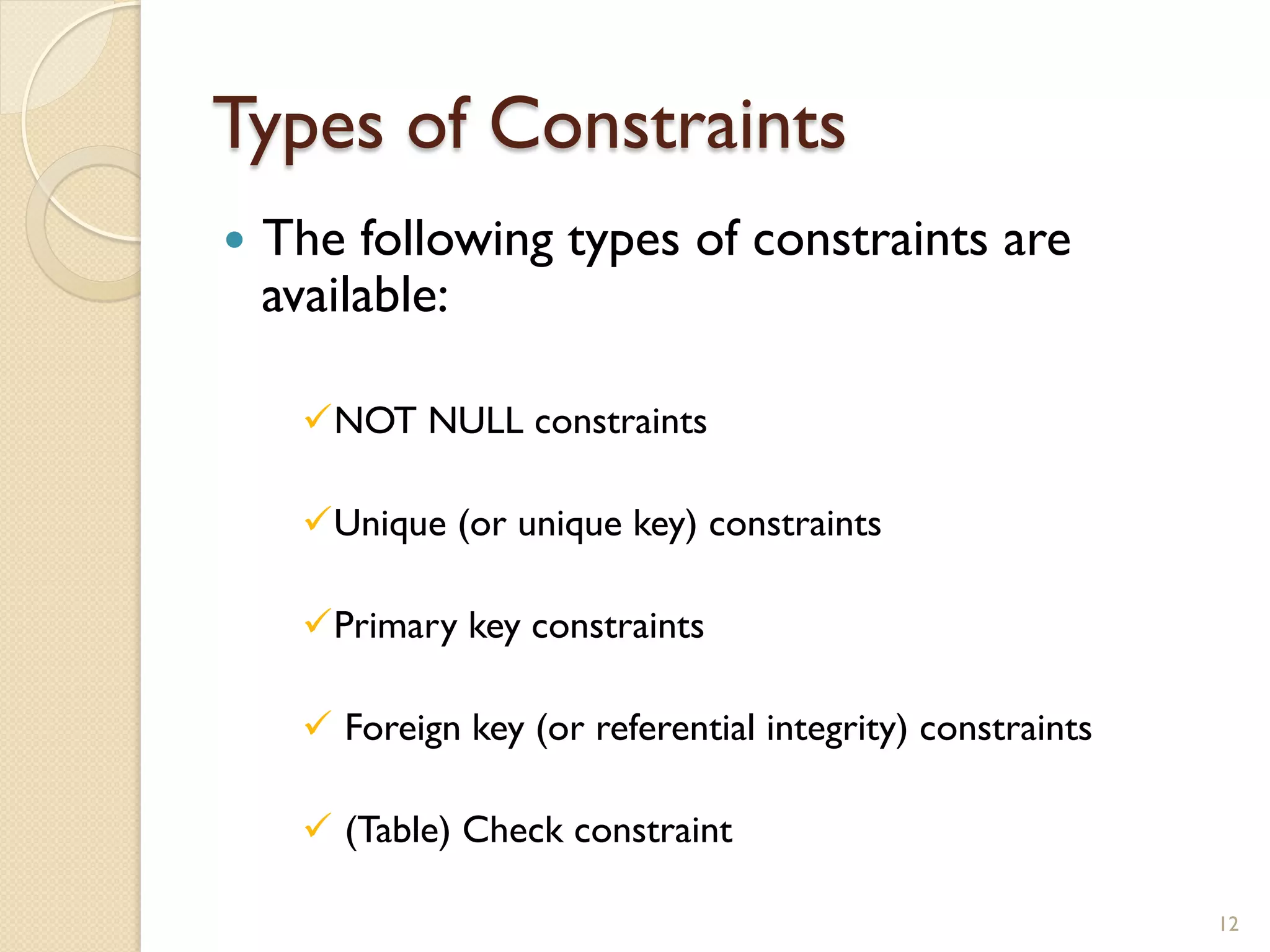
— A schema is a collection of named database objects.
— Schemas provide a way to logically classify objects such as tables,
views, triggers, routines, or packages.
— A schema name is used as the first part of a table.
— A schema is itself a database object that is created using the
CREATE SCHEMA statement. The syntax of the CREATE
SCHEMA statement is as follows:
— CREATE SCHEMA { <schema-name> | AUTHORIZATION
<authorization-name> |
<schema-name> AUTHORIZATION <authorization-name> }
[ <schema-SQL-statement> ... ]o-part object name
27](https://image.slidesharecdn.com/understandingaboutrelationaldatabase-m-squaresystemsinc-141110091320-conversion-gate02/75/Understanding-about-relational-database-m-square-systems-inc-27-2048.jpg)


![Schema
— A schema is a collection of named database objects.
— Schemas provide a way to logically classify objects such as tables,
views, triggers, routines, or packages.
— A schema name is used as the first part of a table.
— A schema is itself a database object that is created using the
CREATE SCHEMA statement. The syntax of the CREATE
SCHEMA statement is as follows:
— CREATE SCHEMA { <schema-name> | AUTHORIZATION
<authorization-name> |
<schema-name> AUTHORIZATION <authorization-name> }
[ <schema-SQL-statement> ... ]o-part object name
27](https://crownmelresort.com/image.slidesharecdn.com/understandingaboutrelationaldatabase-m-squaresystemsinc-141110091320-conversion-gate02/75/Understanding-about-relational-database-m-square-systems-inc-27-2048.jpg)


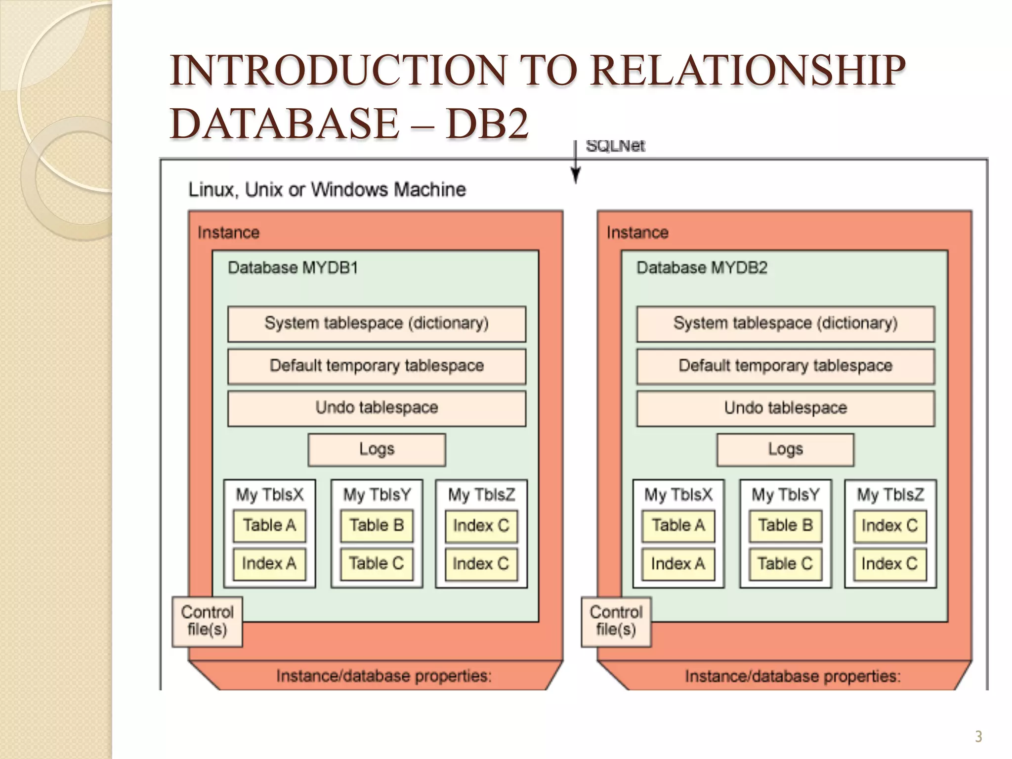
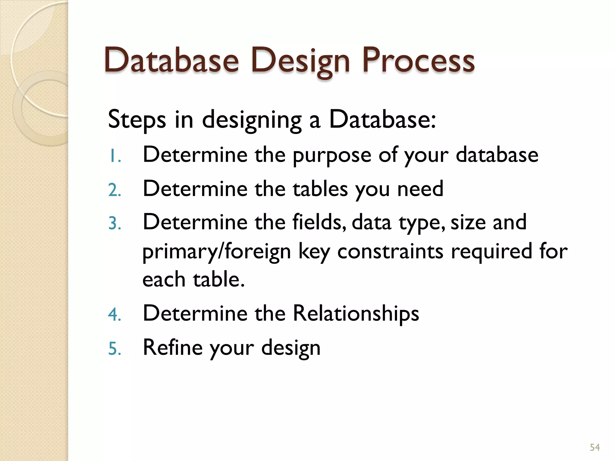
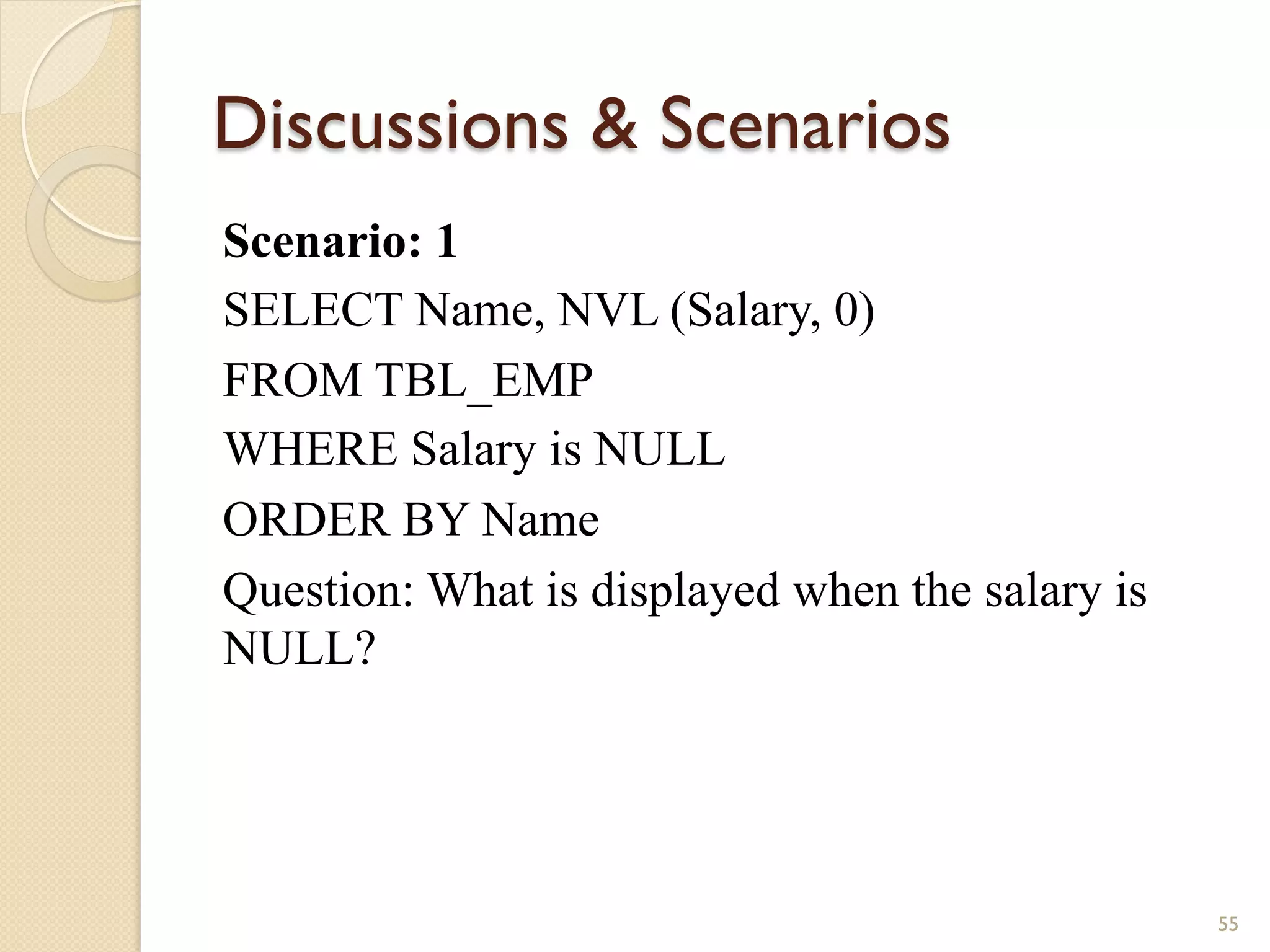
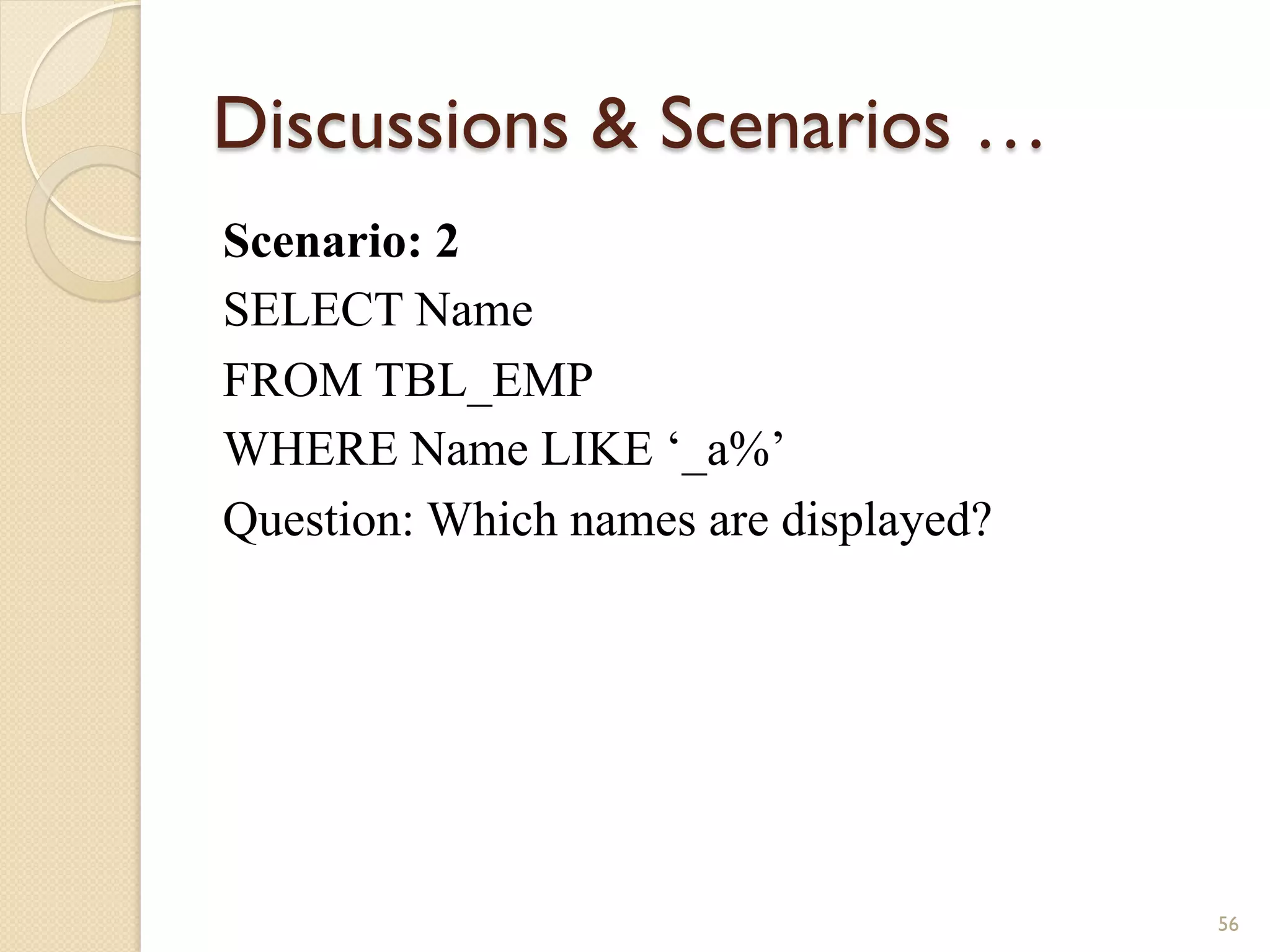
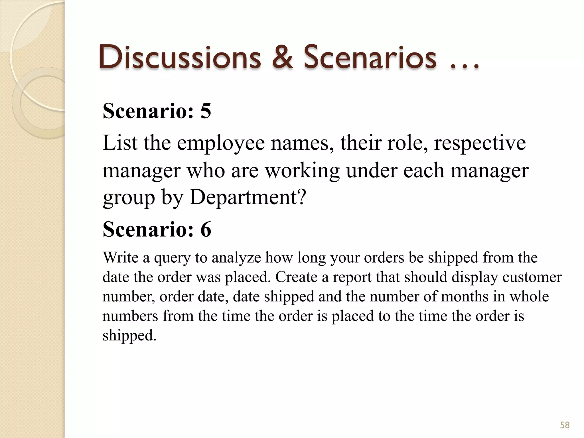
This document provides an in-depth overview of relational database management systems (RDBMS), specifically focusing on IBM DB2. It covers various concepts including types of relationships, normalization, referential integrity, performance optimization, and SQL queries, while detailing design practices and constraints. The document aims to equip users with foundational knowledge required for effective database management and optimization.