Download as PDF, PPTX
![An
Example
1 class Vec {
2 double x, y;
3 sub(v) {
4 res=new Vec(x-v.x, y-v.y);
5 return res;
6 }
7 }
8 for (i = 0; i < N; i++) {
9 t = in[i+2].sub(a[i-1]);
10 q[i] = t;
11 t = in[i+1].sub(a[i-2]);
12 // use of fields of t
13 }
……
80 t=q[*];
81 // use of fields of t
3](https://image.slidesharecdn.com/icse12-120724183252-phpapp01/75/Uncovering-Performance-Problems-in-Java-Applications-with-Reference-Propagation-Profiling-3-2048.jpg)
![An
Example
1 class Vec {
2 double x, y;
3 sub(v) {
4 res=new Vec(x-v.x, y-v.y);
5 return res;
6 }
7 }
8 for (i = 0; i < N; i++) {
9 t = in[i+2].sub(a[i-1]);
10 q[i] = t;
11 t = in[i+1].sub(a[i-2]);
12 // use of fields of t
13 }
……
80 t=q[*];
81 // use of fields of t
4](https://image.slidesharecdn.com/icse12-120724183252-phpapp01/75/Uncovering-Performance-Problems-in-Java-Applications-with-Reference-Propagation-Profiling-4-2048.jpg)
![An
Example
1 class Vec {
2 double x, y;
3 sub(v) {
4 res=new Vec(x-v.x, y-v.y);
5 return res;
6 }
7 }
8 for (i = 0; i < N; i++) {
9 t = in[i+2].sub(a[i-1]);
10 q[i] = t;
11 t = in[i+1].sub(a[i-2]);
12 // use of fields of t
13 }
……
80 t=q[*];
81 // use of fields of t
5](https://image.slidesharecdn.com/icse12-120724183252-phpapp01/75/Uncovering-Performance-Problems-in-Java-Applications-with-Reference-Propagation-Profiling-5-2048.jpg)
![An
Example
1 class Vec {
2 double x, y;
3 sub(v) {
4 res=new Vec(x-v.x, y-v.y);
5 return res;
6 }
7 }
8 for (i = 0; i < N; i++) {
9 t = in[i+2].sub(a[i-1]);
10 q[i] = t;
11 t = in[i+1].sub(a[i-2]);
12 // use of fields of t
13 }
……
80 t=q[*];
81 // use of fields of t
6](https://image.slidesharecdn.com/icse12-120724183252-phpapp01/75/Uncovering-Performance-Problems-in-Java-Applications-with-Reference-Propagation-Profiling-6-2048.jpg)
![An
Example
1 class Vec {
2 double x, y;
3 sub(v) {
4 res=new Vec(x-v.x, y-v.y);
5 return res;
6 }
7 }
8 for (i = 0; i < N; i++) {
9 t = in[i+2].sub(a[i-1]);
10 q[i] = t;
11 t = in[i+1].sub(a[i-2]);
12 // use of fields of t
13 }
……
80 t=q[*];
81 // use of fields of t
7](https://image.slidesharecdn.com/icse12-120724183252-phpapp01/75/Uncovering-Performance-Problems-in-Java-Applications-with-Reference-Propagation-Profiling-7-2048.jpg)
![An
Example
1 class Vec {
2 double x, y;
3 sub(v) {
4 res=new Vec(x-v.x, y-v.y);
5 return res;
6 }
7 }
8 for (i = 0; i < N; i++) {
9 t = in[i+2].sub(a[i-1]);
10 q[i] = t;
11 t = in[i+1].sub(a[i-2]);
12 // use of fields of t
13 }
……
80 t=q[*];
81 // use of fields of t
8](https://image.slidesharecdn.com/icse12-120724183252-phpapp01/75/Uncovering-Performance-Problems-in-Java-Applications-with-Reference-Propagation-Profiling-8-2048.jpg)
![A
Real
Tuning
Session
1 class Vec {
2 double x, y;
3 sub(v) {
4 res=new Vec(x-v.x, y-v.y);
5 return res;
6 }
7 }
8 for (i = 0; i < N; i++) {
9 t = in[i+2].sub(a[i-1]);
10 q[i] = t;
11 t = in[i+1].sub(a[i-2]);
12 // use of fields of t
13 }
……
80 t=q[*];
81 // use of fields of t
20](https://image.slidesharecdn.com/icse12-120724183252-phpapp01/75/Uncovering-Performance-Problems-in-Java-Applications-with-Reference-Propagation-Profiling-20-2048.jpg)
![A
Real
Tuning
Session
1 class Vec {
2 double x, y;
3 sub(v) {
4 res=new Vec(x-v.x, y-v.y);
5 return res;
6 }
7 }
8 for (i = 0; i < N; i++) {
9 t = in[i+2].sub(a[i-1]);
10 q[i] = t;
11 t = in[i+1].sub(a[i-2]);
12 // use of fields of t
13 }
……
80 t=q[*];
81 // use of fields of t
21](https://image.slidesharecdn.com/icse12-120724183252-phpapp01/75/Uncovering-Performance-Problems-in-Java-Applications-with-Reference-Propagation-Profiling-21-2048.jpg)
![A
Real
Tuning
Session
1 class Vec {
2 double x, y;
1 2
3 sub(v) {
4 res=new Vec(x-v.x, y-v.y);
5 return res;
6 }
7 }
8 for (i = 0; i < N; i++) {
9 t = in[i+2].sub(a[i-1]); 1
10 q[i] = t;
11 t = in[i+1].sub(a[i-2]); 2
12 // use of fields of t
13 }
……
80 t=q[*];
81 // use of fields of t
22](https://image.slidesharecdn.com/icse12-120724183252-phpapp01/75/Uncovering-Performance-Problems-in-Java-Applications-with-Reference-Propagation-Profiling-22-2048.jpg)
![A
Real
Tuning
Session
1 class Vec {
2 double x, y;
1 2
3 sub(v) {
4 res=new Vec(x-v.x, y-v.y);
5 return res;
6 }
7 }
8 for (i = 0; i < N; i++) {
9 t = in[i+2].sub(a[i-1]); 1
10 q[i] = t;
11 t = in[i+1].sub(a[i-2]); 2
12 // use of fields of t
13 }
……
80 t=q[*];
81 // use of fields of t
23](https://image.slidesharecdn.com/icse12-120724183252-phpapp01/75/Uncovering-Performance-Problems-in-Java-Applications-with-Reference-Propagation-Profiling-23-2048.jpg)
![A
Real
Tuning
Session
1 class Vec { 1 class Vec {
2 double x, y; 2 double x, y;
3 sub(v) { 3 sub_rev(v, res) {
4 res=new Vec(x-v.x, y-v.y); 4 res.x = x-v.x;
5 return res; 5 res.y = y-v.y;
6 } 6 }
7 } tuning 7 } = new Vec; // reusable
nt
8 for (i = 0; i < N; i++) { 8 for (i = 0; i < N; i++) {
9 t = in[i+2].sub(a[i-1]); 9 t = in[i+2].sub(a[i-1]);
10 q[i] = t; 10 q[i] = t;
11 t = in[i+1].sub(a[i-2]); 11 in[i+1].sub_rev(a[i-2], nt);
12 // use of fields of t 12 // use of fields of nt
13 } 13 }
…… ……
80 t=q[*]; 80 t=q[*];
81 // use of fields of t 81 // use of fields of t
24](https://image.slidesharecdn.com/icse12-120724183252-phpapp01/75/Uncovering-Performance-Problems-in-Java-Applications-with-Reference-Propagation-Profiling-24-2048.jpg)
![A
Real
Tuning
Session
1 class Vec { 1 class Vec {
2 double x, y; 2 double x, y;
3 sub(v) { 3 sub_rev(v, res) {
4 res=new Vec(x-v.x, y-v.y); 4 res.x = x-v.x;
5 return res; 5 res.y = y-v.y;
6 } 6 }
7 } tuning 7 } = new Vec; // reusable
nt
8 for (i = 0; i < N; i++) { 8 for (i = 0; i < N; i++) {
9 t = in[i+2].sub(a[i-1]); 9 t = in[i+2].sub(a[i-1]);
10 q[i] = t; 10 q[i] = t;
11 t = in[i+1].sub(a[i-2]); 11 in[i+1].sub_rev(a[i-2], nt);
12 // use of fields of t 12 // use of fields of nt
13 } 13 }
…… ……
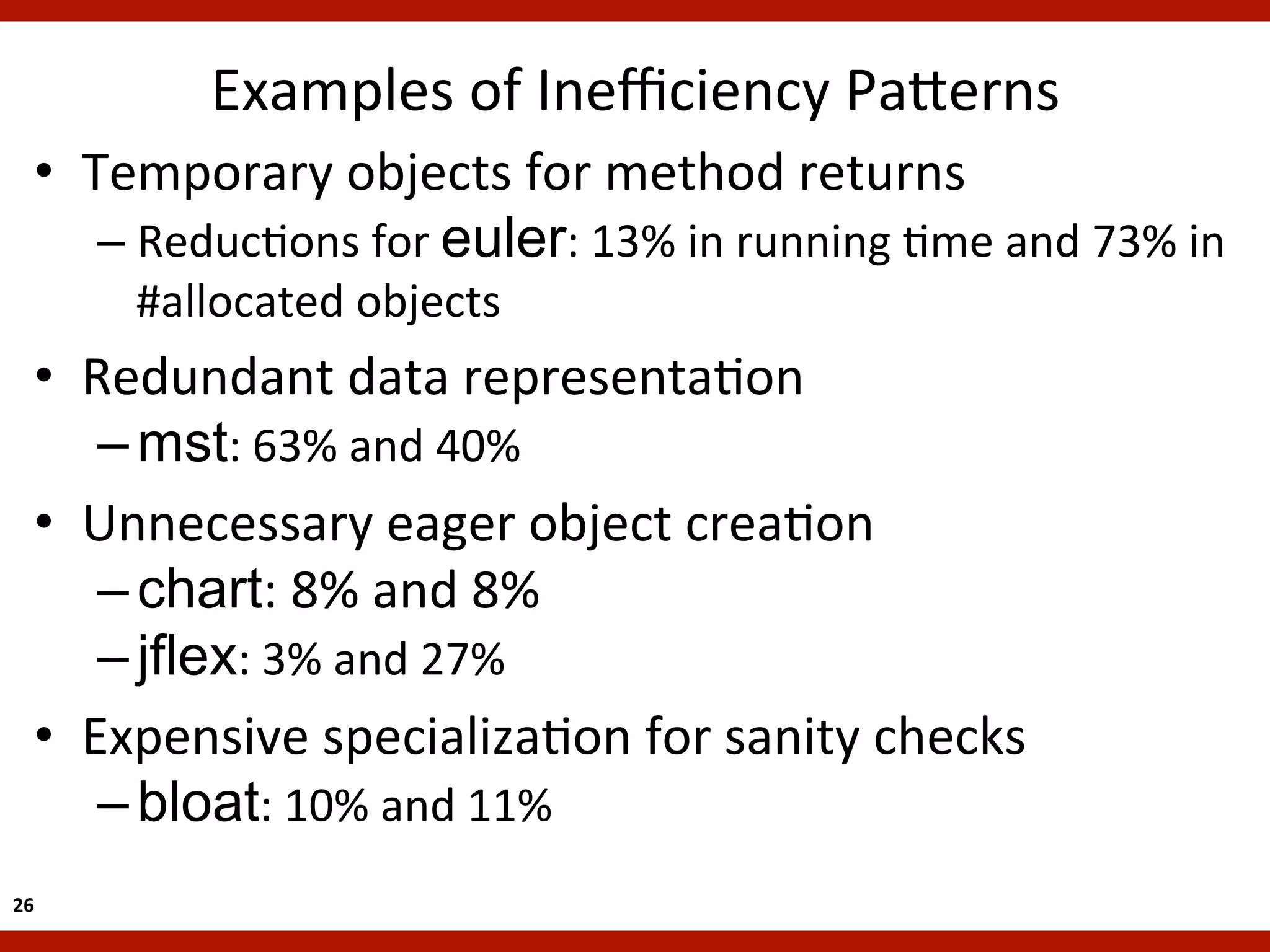
80 t=q[*]; Reductions: 13% in running time and
80 t=q[*];
81 // use of fields of t 73% in #allocated objectsof fields of t
81 // use
25](https://image.slidesharecdn.com/icse12-120724183252-phpapp01/75/Uncovering-Performance-Problems-in-Java-Applications-with-Reference-Propagation-Profiling-25-2048.jpg)


![An
Example
1 class Vec {
2 double x, y;
3 sub(v) {
4 res=new Vec(x-v.x, y-v.y);
5 return res;
6 }
7 }
8 for (i = 0; i < N; i++) {
9 t = in[i+2].sub(a[i-1]);
10 q[i] = t;
11 t = in[i+1].sub(a[i-2]);
12 // use of fields of t
13 }
……
80 t=q[*];
81 // use of fields of t
3](https://crownmelresort.com/image.slidesharecdn.com/icse12-120724183252-phpapp01/75/Uncovering-Performance-Problems-in-Java-Applications-with-Reference-Propagation-Profiling-3-2048.jpg)
![An
Example
1 class Vec {
2 double x, y;
3 sub(v) {
4 res=new Vec(x-v.x, y-v.y);
5 return res;
6 }
7 }
8 for (i = 0; i < N; i++) {
9 t = in[i+2].sub(a[i-1]);
10 q[i] = t;
11 t = in[i+1].sub(a[i-2]);
12 // use of fields of t
13 }
……
80 t=q[*];
81 // use of fields of t
4](https://crownmelresort.com/image.slidesharecdn.com/icse12-120724183252-phpapp01/75/Uncovering-Performance-Problems-in-Java-Applications-with-Reference-Propagation-Profiling-4-2048.jpg)
![An
Example
1 class Vec {
2 double x, y;
3 sub(v) {
4 res=new Vec(x-v.x, y-v.y);
5 return res;
6 }
7 }
8 for (i = 0; i < N; i++) {
9 t = in[i+2].sub(a[i-1]);
10 q[i] = t;
11 t = in[i+1].sub(a[i-2]);
12 // use of fields of t
13 }
……
80 t=q[*];
81 // use of fields of t
5](https://crownmelresort.com/image.slidesharecdn.com/icse12-120724183252-phpapp01/75/Uncovering-Performance-Problems-in-Java-Applications-with-Reference-Propagation-Profiling-5-2048.jpg)
![An
Example
1 class Vec {
2 double x, y;
3 sub(v) {
4 res=new Vec(x-v.x, y-v.y);
5 return res;
6 }
7 }
8 for (i = 0; i < N; i++) {
9 t = in[i+2].sub(a[i-1]);
10 q[i] = t;
11 t = in[i+1].sub(a[i-2]);
12 // use of fields of t
13 }
……
80 t=q[*];
81 // use of fields of t
6](https://crownmelresort.com/image.slidesharecdn.com/icse12-120724183252-phpapp01/75/Uncovering-Performance-Problems-in-Java-Applications-with-Reference-Propagation-Profiling-6-2048.jpg)
![An
Example
1 class Vec {
2 double x, y;
3 sub(v) {
4 res=new Vec(x-v.x, y-v.y);
5 return res;
6 }
7 }
8 for (i = 0; i < N; i++) {
9 t = in[i+2].sub(a[i-1]);
10 q[i] = t;
11 t = in[i+1].sub(a[i-2]);
12 // use of fields of t
13 }
……
80 t=q[*];
81 // use of fields of t
7](https://crownmelresort.com/image.slidesharecdn.com/icse12-120724183252-phpapp01/75/Uncovering-Performance-Problems-in-Java-Applications-with-Reference-Propagation-Profiling-7-2048.jpg)
![An
Example
1 class Vec {
2 double x, y;
3 sub(v) {
4 res=new Vec(x-v.x, y-v.y);
5 return res;
6 }
7 }
8 for (i = 0; i < N; i++) {
9 t = in[i+2].sub(a[i-1]);
10 q[i] = t;
11 t = in[i+1].sub(a[i-2]);
12 // use of fields of t
13 }
……
80 t=q[*];
81 // use of fields of t
8](https://crownmelresort.com/image.slidesharecdn.com/icse12-120724183252-phpapp01/75/Uncovering-Performance-Problems-in-Java-Applications-with-Reference-Propagation-Profiling-8-2048.jpg)


![A
Real
Tuning
Session
1 class Vec {
2 double x, y;
3 sub(v) {
4 res=new Vec(x-v.x, y-v.y);
5 return res;
6 }
7 }
8 for (i = 0; i < N; i++) {
9 t = in[i+2].sub(a[i-1]);
10 q[i] = t;
11 t = in[i+1].sub(a[i-2]);
12 // use of fields of t
13 }
……
80 t=q[*];
81 // use of fields of t
20](https://crownmelresort.com/image.slidesharecdn.com/icse12-120724183252-phpapp01/75/Uncovering-Performance-Problems-in-Java-Applications-with-Reference-Propagation-Profiling-20-2048.jpg)
![A
Real
Tuning
Session
1 class Vec {
2 double x, y;
3 sub(v) {
4 res=new Vec(x-v.x, y-v.y);
5 return res;
6 }
7 }
8 for (i = 0; i < N; i++) {
9 t = in[i+2].sub(a[i-1]);
10 q[i] = t;
11 t = in[i+1].sub(a[i-2]);
12 // use of fields of t
13 }
……
80 t=q[*];
81 // use of fields of t
21](https://crownmelresort.com/image.slidesharecdn.com/icse12-120724183252-phpapp01/75/Uncovering-Performance-Problems-in-Java-Applications-with-Reference-Propagation-Profiling-21-2048.jpg)
![A
Real
Tuning
Session
1 class Vec {
2 double x, y;
1 2
3 sub(v) {
4 res=new Vec(x-v.x, y-v.y);
5 return res;
6 }
7 }
8 for (i = 0; i < N; i++) {
9 t = in[i+2].sub(a[i-1]); 1
10 q[i] = t;
11 t = in[i+1].sub(a[i-2]); 2
12 // use of fields of t
13 }
……
80 t=q[*];
81 // use of fields of t
22](https://crownmelresort.com/image.slidesharecdn.com/icse12-120724183252-phpapp01/75/Uncovering-Performance-Problems-in-Java-Applications-with-Reference-Propagation-Profiling-22-2048.jpg)
![A
Real
Tuning
Session
1 class Vec {
2 double x, y;
1 2
3 sub(v) {
4 res=new Vec(x-v.x, y-v.y);
5 return res;
6 }
7 }
8 for (i = 0; i < N; i++) {
9 t = in[i+2].sub(a[i-1]); 1
10 q[i] = t;
11 t = in[i+1].sub(a[i-2]); 2
12 // use of fields of t
13 }
……
80 t=q[*];
81 // use of fields of t
23](https://crownmelresort.com/image.slidesharecdn.com/icse12-120724183252-phpapp01/75/Uncovering-Performance-Problems-in-Java-Applications-with-Reference-Propagation-Profiling-23-2048.jpg)
![A
Real
Tuning
Session
1 class Vec { 1 class Vec {
2 double x, y; 2 double x, y;
3 sub(v) { 3 sub_rev(v, res) {
4 res=new Vec(x-v.x, y-v.y); 4 res.x = x-v.x;
5 return res; 5 res.y = y-v.y;
6 } 6 }
7 } tuning 7 } = new Vec; // reusable
nt
8 for (i = 0; i < N; i++) { 8 for (i = 0; i < N; i++) {
9 t = in[i+2].sub(a[i-1]); 9 t = in[i+2].sub(a[i-1]);
10 q[i] = t; 10 q[i] = t;
11 t = in[i+1].sub(a[i-2]); 11 in[i+1].sub_rev(a[i-2], nt);
12 // use of fields of t 12 // use of fields of nt
13 } 13 }
…… ……
80 t=q[*]; 80 t=q[*];
81 // use of fields of t 81 // use of fields of t
24](https://crownmelresort.com/image.slidesharecdn.com/icse12-120724183252-phpapp01/75/Uncovering-Performance-Problems-in-Java-Applications-with-Reference-Propagation-Profiling-24-2048.jpg)
![A
Real
Tuning
Session
1 class Vec { 1 class Vec {
2 double x, y; 2 double x, y;
3 sub(v) { 3 sub_rev(v, res) {
4 res=new Vec(x-v.x, y-v.y); 4 res.x = x-v.x;
5 return res; 5 res.y = y-v.y;
6 } 6 }
7 } tuning 7 } = new Vec; // reusable
nt
8 for (i = 0; i < N; i++) { 8 for (i = 0; i < N; i++) {
9 t = in[i+2].sub(a[i-1]); 9 t = in[i+2].sub(a[i-1]);
10 q[i] = t; 10 q[i] = t;
11 t = in[i+1].sub(a[i-2]); 11 in[i+1].sub_rev(a[i-2], nt);
12 // use of fields of t 12 // use of fields of nt
13 } 13 }
…… ……
80 t=q[*]; Reductions: 13% in running time and
80 t=q[*];
81 // use of fields of t 73% in #allocated objectsof fields of t
81 // use
25](https://crownmelresort.com/image.slidesharecdn.com/icse12-120724183252-phpapp01/75/Uncovering-Performance-Problems-in-Java-Applications-with-Reference-Propagation-Profiling-25-2048.jpg)


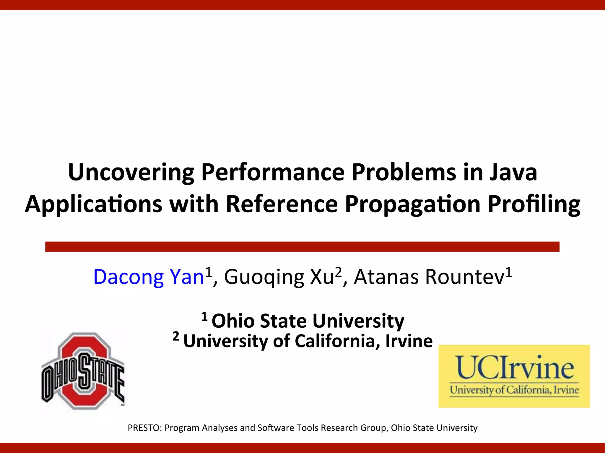
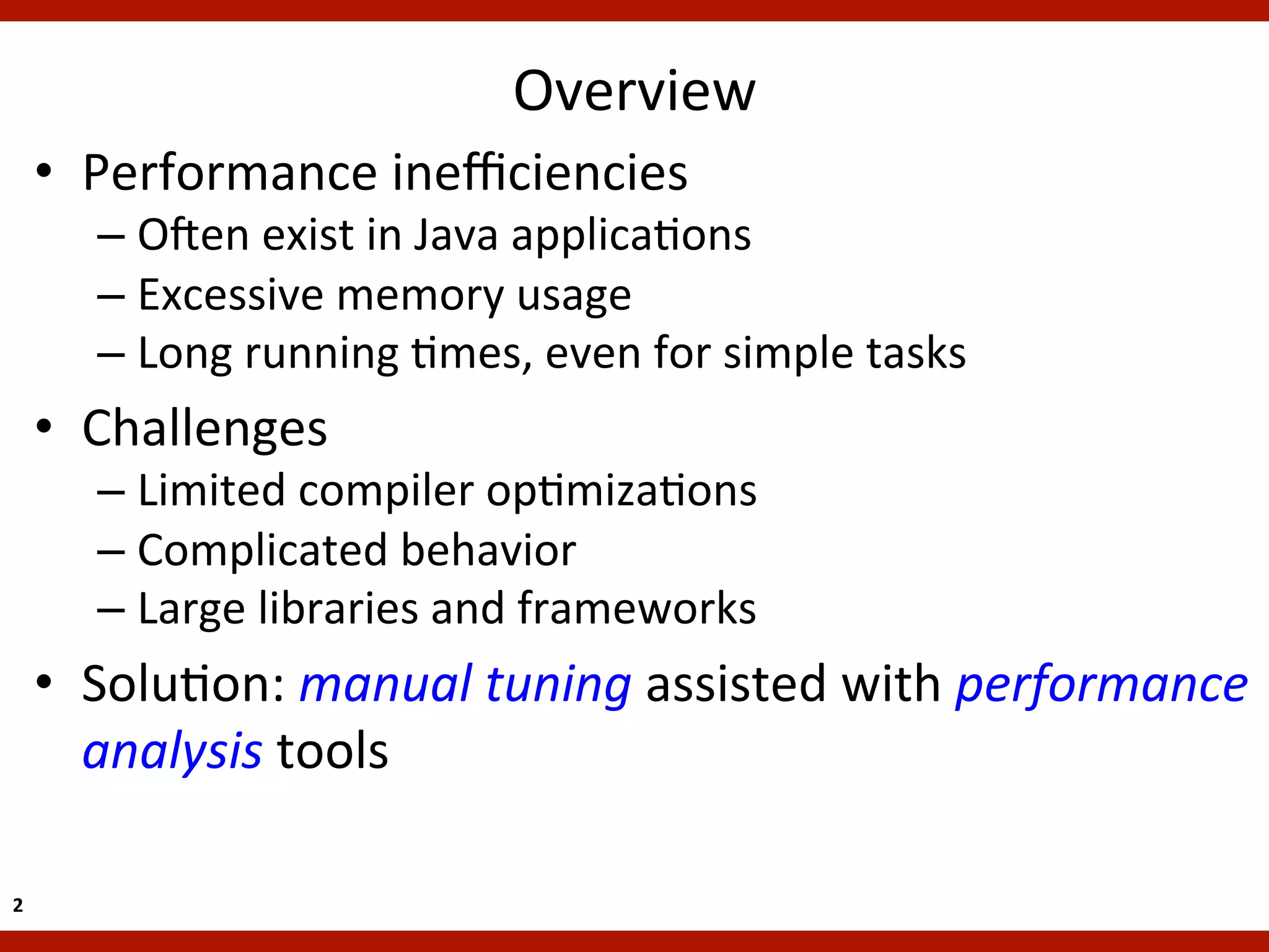
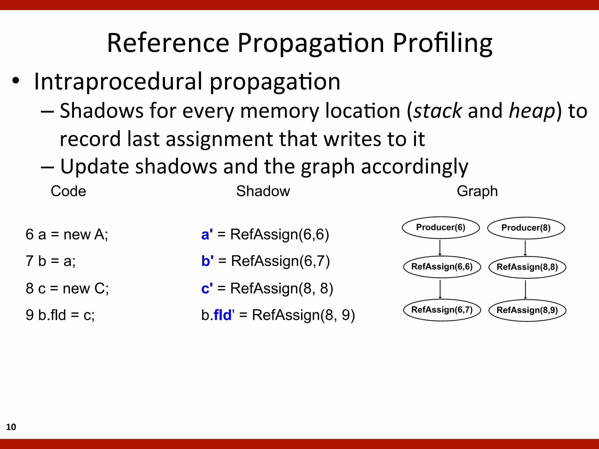
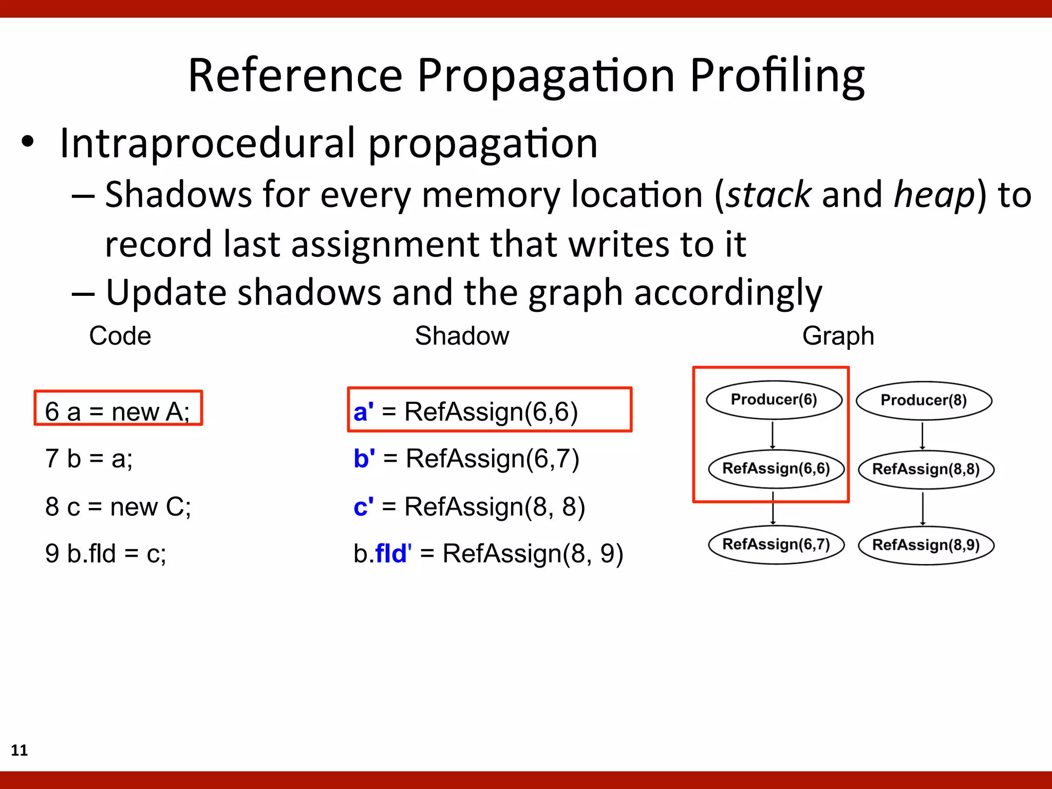
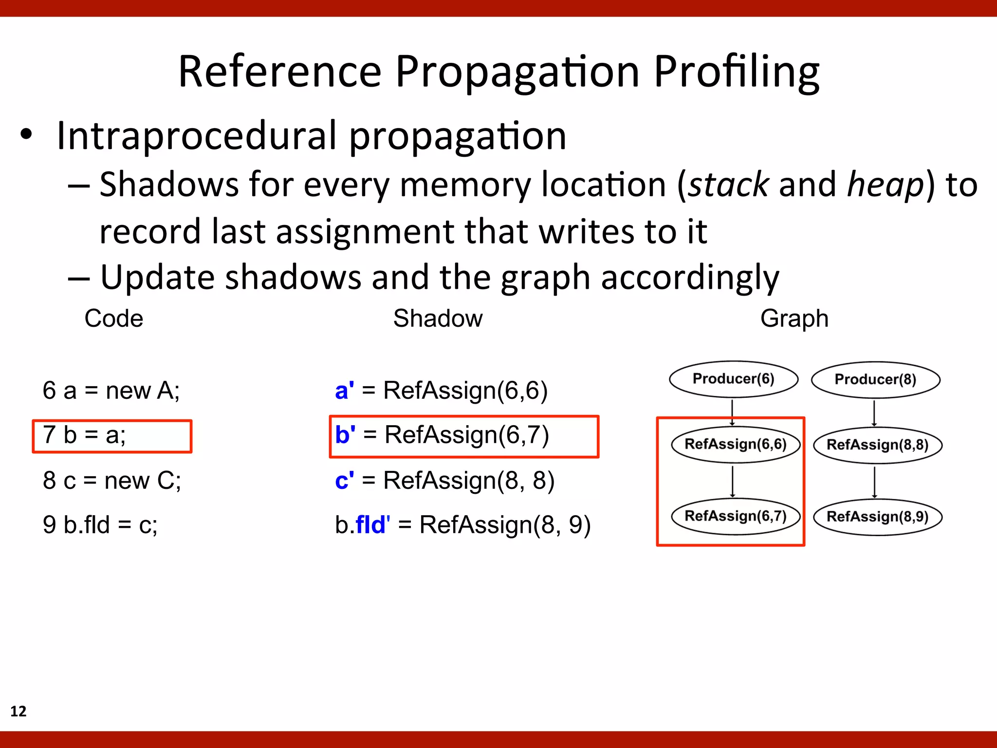
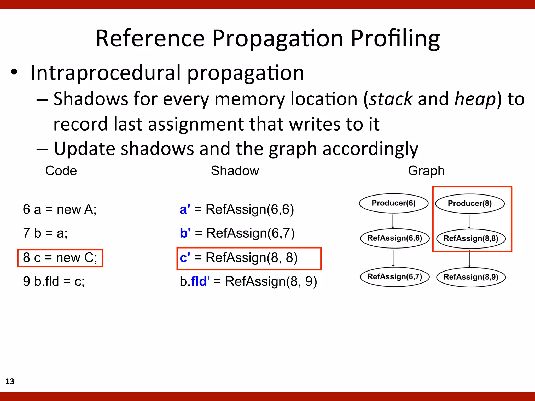
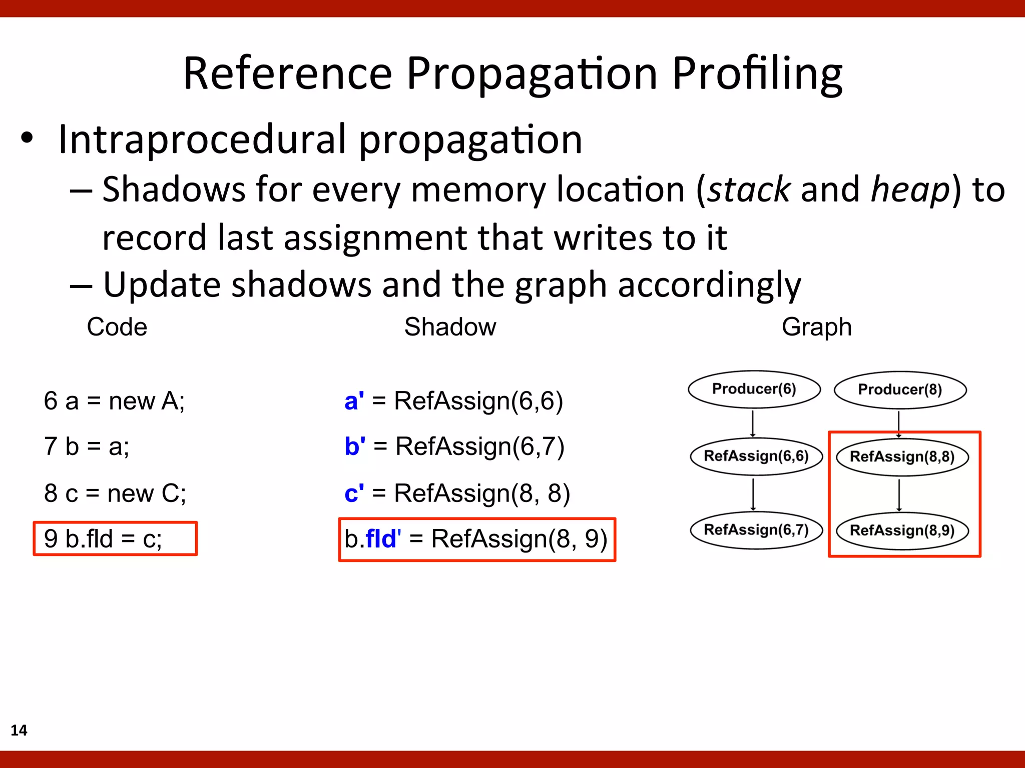
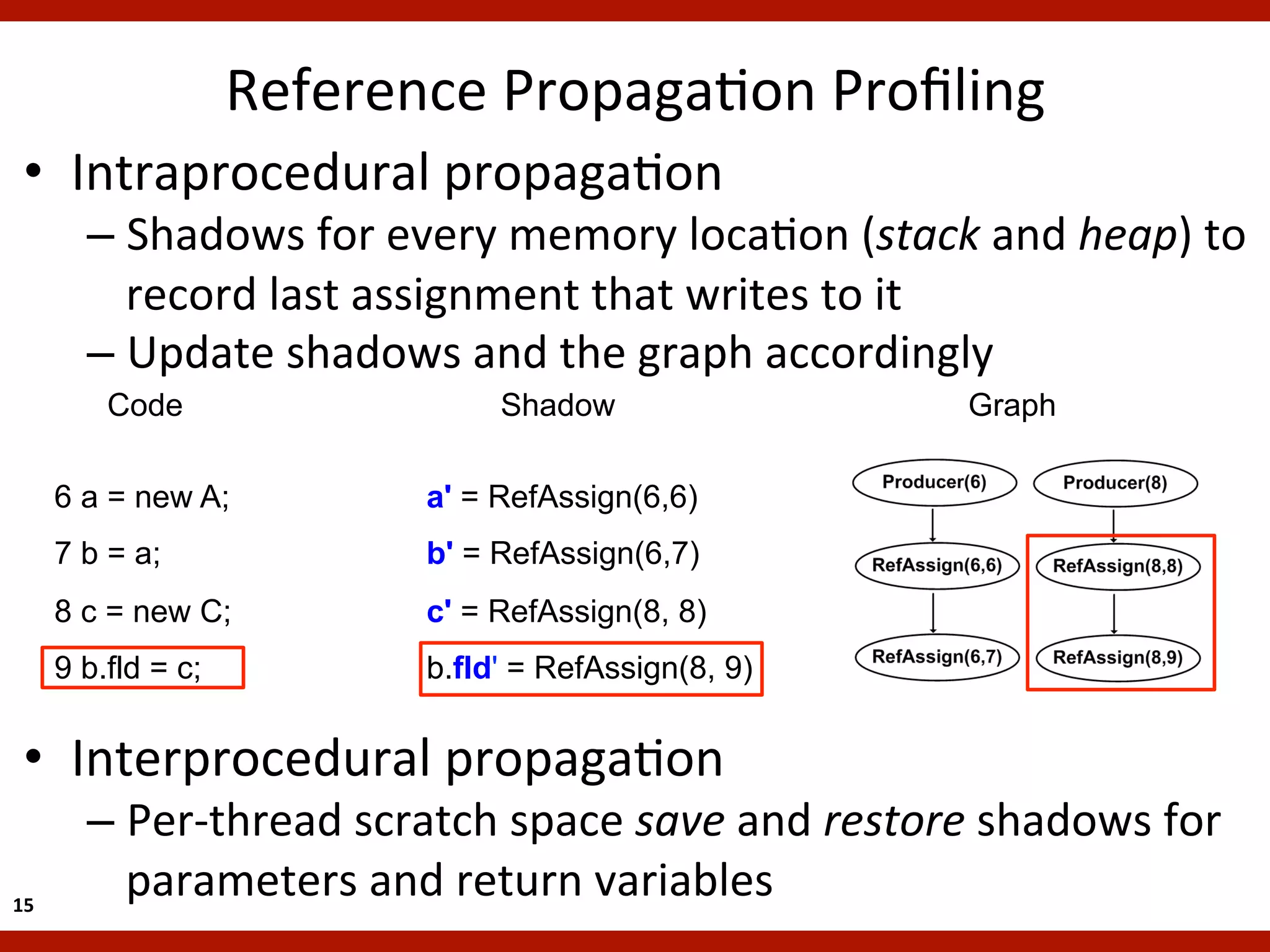
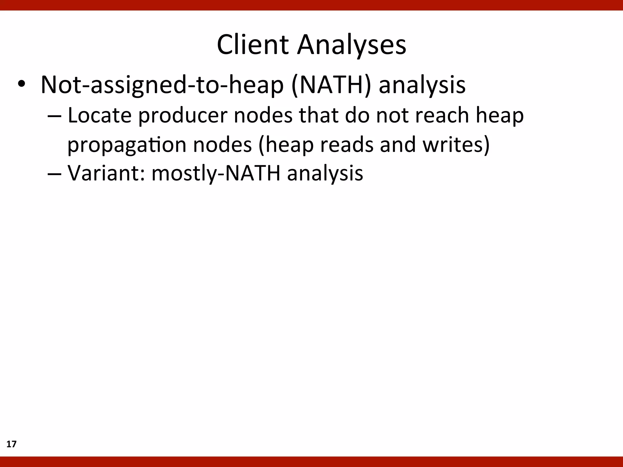
The document discusses reference propagation profiling, a technique for uncovering performance problems in Java applications. It is implemented in the Jikes RVM compiler by instrumenting code to track data dependencies and propagate references between memory locations. This allows analyzing applications to find inefficiencies like objects not being assigned to the heap or imbalance between operation costs and benefits. The profiling has high overhead but provides insights to assist with manual performance tuning.