Download to read offline
![JCAP12(2024)022
Contents
1 Introduction 1
2 Data 3
2.1 DESI Luminous Red Galaxy sample 3
2.2 CMB lensing 5
3 CMB lensing tomography measurement 7
3.1 Angular power spectrum 9
3.2 Simulations 12
3.3 Transfer function 13
3.4 Covariance matrix 15
4 Systematics and null tests 18
4.1 Foreground contamination assessment 18
4.2 Null tests 20
5 Cosmological constraints and analysis 25
5.1 Blinding policy 25
5.2 Theory model 27
5.3 Cosmological parameterization and priors 27
5.4 Parameter inference 28
5.5 Parameter recovery tests 29
5.6 Results 30
6 Summary and discussion 33
A Null test plots 36
B SNR calculation 36
Author List 45
1 Introduction
The standard cosmological model, featuring cold dark matter (CDM) and a cosmological
constant Λ, has been largely successful in describing how primordial density fluctuations
developed into the present-day matter distribution. Our picture of the early universe is
informed by the primary anisotropies in the cosmic microwave background (CMB) [1–4],
which consists of radiation from the epoch of recombination at z ≈ 1100. As these photons
pass through gravitational potentials on their journey to us, they are deflected due to
gravitational lensing (e.g., [5]) allowing the CMB to be used as a probe of the late-time matter
distribution as well. Together with complementary probes of the late universe including
– 1 –](https://image.slidesharecdn.com/kim2024j-250202225338-b52a3653/75/The-Atacama-Cosmology-Telescope-DR6-and-DESI-structure-formation-over-cosmic-time-with-a-measurement-of-the-cross-correlation-of-CMB-lensing-and-luminous-red-galaxies-3-2048.jpg)
![JCAP12(2024)022
galaxy clustering [6–8], cluster cosmology [9, 10] and galaxy weak lensing [11–20], a suite of
observables have reached the precision required to informatively compare with the prediction
from early-universe CMB measurements.
The matter distribution is typically characterized in terms of σ8, the amplitude of matter
density fluctuations smoothed on a scale of 8 Mpc/h. Weak lensing observables, in particular,
measure degenerate combinations with the average matter density of the universe Ωm, e.g.,
S8 = σ8
p
Ωm/0.3. Early observations of galaxy lensing with the CFHTLens survey [21] began
to hint at a possible disagreement of this quantity between direct late-time observables and
the primary CMB prediction [22–24]. Today, primary CMB measurements provide strong
constraints on S8 (derived through extrapolation to late times and assuming the ΛCDM
model), e.g., S8 = 0.834 ± 0.016 from Planck 2018 (PR3) [1], S8 = 0.827 ± 0.013 from
Planck NPIPE (PR4) [2], S8 = 0.830 ± 0.043 from ACT DR4 [3], and S8 = 0.797 ± 0.042 from
the South Pole Telescope (SPT-3G, [4]) while measurements of the combination of galaxy weak
lensing and galaxy clustering from surveys such as the Dark Energy Survey (DES, [11, 12]), the
Kilo-Degree Survey (KiDS, [13, 14]), and the Hyper Suprime-Cam (HSC, [15–18]) typically
tend to find lower values, S8 = 0.776 ± 0.017, S8 = 0.765+0.017
−0.016, and S8 = 0.775+0.043
−0.038
respectively. Low inferences are also found in full-shape analyses of galaxy clustering from
the Baryon Oscillation Spectroscopic Survey (BOSS, e.g., [7, 25]), but clustering from the full
Sloan Digital Sky Survey (SDSS, [26]) that includes BOSS data as well as the joint reanalysis
of galaxy weak lensing data from DES Y3 and KiDS-1000 [27] find slightly higher values.
Intriguingly, measurements of the CMB lensing power spectrum that best infer properties of
structure at intermediate redshifts 0.5 < z < 5 [28] are in good agreement with the primary
CMB: S8 = 0.831 ± 0.029 from Planck PR41 [29], S8 = 0.840 ± 0.028 from ACT DR6 [28, 30]
and S8 = 0.836 ± 0.039 from SPT-3G [31]. Galaxy cluster abundance measured by SPT ([10])
gives an intermediate value of S8 = 0.795 ± 0.029, while an analysis using the first eROSITA
All-Sky Survey (eRASS1, [9]) presents a higher value of S8 = 0.86 ± 0.01.
Discrepancies between various probes could be sourced by systematics (e.g., unaccounted
for baryonic feedback on small scales [32, 33]), due to new physics (see e.g., [34]), or caused
by statistical fluctuations. Disentangling these requires observables across a range of redshifts
and comoving wave-numbers, as well as observations that constrain feedback, e.g., [35, 36].
In this context, the cross-correlation of CMB lensing with the galaxy distribution can provide
insight by exploring a wide range of redshifts while minimizing sensitivity to uncertainties on
small scales. Recent galaxy-CMB lensing cross-correlation analyses show varying results: the
cross-correlation of DES Y3 MagLim galaxies with ACT DR4 CMB lensing [37] constrains
S8 = 0.75+0.04
−0.05, the cross-correlation of BOSS with Planck PR3 [38] yields S8 = 0.707 ± 0.037,
the cross-correlation of DES Y3 with SPT-SZ and Planck PR3 [39] presents S8 = 0.736+0.032
−0.028,
while the cross-correlation of unWISE galaxies with the newer ACT DR6 CMB lensing and
Planck PR4 [40] shows S8 = 0.805 ± 0.018.
Cross-correlations with spectroscopically calibrated galaxy samples, in particular, have
the potential to add significant additional robustness to tomographic studies. The Dark
Energy Spectroscopic Instrument (DESI) survey [41–48] has collected O(106) redshifts which
1
The value of S8 from Planck PR4 lensing was not explicitly provided in [29] but rather inferred from the
chains provided in section IV: https://github.com/carronj/planck_PR4_lensing.
– 2 –](https://image.slidesharecdn.com/kim2024j-250202225338-b52a3653/75/The-Atacama-Cosmology-Telescope-DR6-and-DESI-structure-formation-over-cosmic-time-with-a-measurement-of-the-cross-correlation-of-CMB-lensing-and-luminous-red-galaxies-4-2048.jpg)
![JCAP12(2024)022
we use here to calibrate the redshift distribution of target galaxies from the DESI Legacy
Imaging Surveys [49]. A previous Planck CMB lensing cross-correlation analysis [50] used a
similarly calibrated DESI sample and found a value of S8 = 0.73 ± 0.03 that is discrepant
with the CMB prediction at ∼ 3σ. In this work, we include lensing maps from the Atacama
Cosmology Telescope (ACT) Data Release 6 (DR6), along with newer Planck CMB lensing
maps from PR4 as well as several improvements to the analysis and theory modeling.
This paper is one of two papers along with [51] analyzing the tomographic cross-correlation
between ACT DR6 CMB lensing and the DESI luminous red galaxies (LRGs). In our
companion paper [51], we delve into further details of the galaxy sample, discuss the HEFT
model used in the analysis, and present constraints on S8 and σ8 when combining with
baryon acoustic oscillation (BAO) data. This paper details the methods and systematics in
computing the galaxy-CMB lensing cross-correlation signal as an angular power spectrum and
combines that with the DESI LRG auto-correlation angular power spectrum measurement to
break the galaxy bias degeneracy. To demonstrate the constraining power of our analysis,
this paper reports our best-constrained amplitude parameter S×
8 = σ8(Ωm/0.3)0.4 (with a
slightly different exponent from S8), including as a function of redshift.
The outline of this paper is as follows: section 2 discusses the CMB lensing and LRG
data used in this analysis, section 3 details the cross-correlation measurement computed
with this data, section 3.2 describes the generation and usage of simulations, including the
calculation of the multiplicative transfer function in section 3.3, and the formulation of the
analysis covariance matrix is described in section 3.4. Various null and consistency tests of
our data and spectra are discussed in section 4. The cosmological parameter inference is
described in section 5, and finally, discussion of the results is presented in section 5.6.
2 Data
In this work, we cross-correlate a sample of luminous red galaxies (LRGs) from the DESI
survey with lensing mass maps from ACT DR6 as well as Planck PR4, with the respective
footprints shown in figure 1. In section 2.1, we briefly summarize the properties of the galaxy
sample from [52, 53] that is used in this analysis, and point the reader to the companion
paper [51] for further details. In section 2.2.1 and section 2.2.2, we describe the CMB
lensing data sets from ACT DR6 [28, 30] and Planck PR4 [29] respectively and how they
will be used for this analysis.
2.1 DESI Luminous Red Galaxy sample
The galaxy data used in this analysis is the “Main LRG” sample from [52], selected from DESI
Legacy Imaging Surveys Data Release 9 (DESI-LS, DR9) photometric data with redshift
distributions calibrated using the DESI Survey Validation (SV) dataset and Early Data
Release [54, 55]. DESI-LS is an imaging survey to provide targets for DESI that consists of (a)
galaxies lying north of declination 32.375◦ sourced from observations by the Beijing-Arizona
Sky Survey (BASS) of the Kitt Peak National Observatory and the Mayall z-band Legacy
Survey of the Mayall Telescope, as well as (b) galaxies lying south of that declination covered
by the Dark Energy Camera (DECam), with DECam providing imaging data to both the
Dark Energy Camera Legacy Survey (DECaLS) and the Dark Energy Survey (DES). To
– 3 –](https://image.slidesharecdn.com/kim2024j-250202225338-b52a3653/75/The-Atacama-Cosmology-Telescope-DR6-and-DESI-structure-formation-over-cosmic-time-with-a-measurement-of-the-cross-correlation-of-CMB-lensing-and-luminous-red-galaxies-5-2048.jpg)
![JCAP12(2024)022
0
30
60
90
120
150 -150
-120
-90
-60
-30
0
R.A. [deg]
-60
-45
-30
-15
0
15
30
45
60
75
Dec
[deg]
Figure 1. The Wiener filtered lensing convergence maps from Planck PR4 (blurry, background)
and ACT DR6 (sharp, foreground) are shown here in equatorial coordinates, with the complete LRG
footprint from DESI-LS shown as a black outline. The joint footprint between ACT and DESI spans
approximately 19% of the full sky (Planck and DESI cover ≈ 44% jointly), with the mutually excluded
region shown in gray surrounding the Galactic plane.
see overlaps between imaging regions contributed from these different surveys, we refer the
reader to figure 2 of [51] — these regions combined lead to a total imaging area of 18,200
deg2 after appropriate cleaning and masking steps.
The “Main LRG” sample is selected and subdivided into four galaxy redshift bins by
their photometric redshifts (photo-z) with criteria detailed in [52] (e.g., total number density
of around 550 deg−2
for all redshift bins combined), but have redshift distributions calibrated
with great precision by 2.3 million spectroscopic redshifts from DESI’s SV and Year 1 data
that are weighted and corrected for redshift failures (see [51, 53]). The photo-z are computed
using a random forest regression on training data from DESI spectroscopic redshifts, Sloan
Digital Sky Survey’s DR16, and a variety of other sources listed in appendix B of [52]. The
redshift distributions of our bins are shown in figure 2.
Before overdensity maps are created, a series of quality cuts were applied to the galaxy
catalog that lead to a cleaned sample with a redshift failure rate of approximately 1% and a
stellar contamination fraction of 0.3% (further details can be seen in [51, 52]). As described
in [52], multiplicative systematic weights for depth and seeing (in the g, r, z bands) as well as
an E(B − V ) correction for Galactic extinction [56] are estimated and applied to a catalog of
random galaxies generated in the DESI footprint.2 Each of the galaxies in the four redshift
bins as well as the randoms are then histogram-binned into a HEALPix map according to their
coordinates, with the overdensity computed as the mean-subtracted galaxy counts map divided
2
Correlations between our E(B − V ) map and large-scale structure have been noted in [52]; however, we
investigate and observe in figure 10 of [51] that these correlations should have little to no impact in our analysis.
– 4 –](https://image.slidesharecdn.com/kim2024j-250202225338-b52a3653/75/The-Atacama-Cosmology-Telescope-DR6-and-DESI-structure-formation-over-cosmic-time-with-a-measurement-of-the-cross-correlation-of-CMB-lensing-and-luminous-red-galaxies-6-2048.jpg)
![JCAP12(2024)022
0.2 0.4 0.6 0.8 1.0 1.2
z
0
2
4
6
8
10
dN
(z)
/
dz
Bin 1
Bin 2
Bin 3
Bin 4
101
102
103
L
0.0
0.5
1.0
1.5
2.0
2.5
3.0
3.5
4.0
10
7
C
κκ
L
PR4 only
Planck PR3 CMB aniso. prediction
Planck PR4 (NPIPE) noise spectrum
Planck PR4 (NPIPE) Cκg
L relative SNR
ACT DR6 noise spectrum
ACT DR6 Cκg
L relative SNR
Figure 2. Left: the redshift distribution dN(z)/dz of the DESI LRG galaxy redshift bins with the CMB
lensing kernel shown in gray, showing ample overlap in redshifts between the two sets of cosmological
probes. Right: Planck CMB prediction for the lensing power spectrum plotted against the lensing noise
spectra of Planck PR4 (shown in blue) and ACT DR6 (shown in red). The lightly shaded bars in colors
represent the fractional contribution to the cross-correlation Cκg
L signal-to-noise using covariances for
Planck PR4 (blue) and ACT DR6 (red) and the same fiducial theory for both (see appendix B for more
details), showing us that Planck holds more constraining power than ACT until L ≈ 400. The shaded
bars in gray show angular multipoles excluded due to scale cuts chosen for the analysis (where the light
gray band labeled “PR4 only” denotes an L band included only for the Planck PR4 cross-correlation).
Both: the colored bars and contours for both figures in addition to the gray CMB lensing kernel in
the left figure are scaled to some arbitrary normalization factor for ease of visualization.
by the weighted random counts map. The resulting DESI galaxy overdensity map and binary
mask for each redshift bin are provided without any modifications from section 7 of [52].3
2.2 CMB lensing
2.2.1 ACT DR6
Our cross-correlation with DESI LRGs uses the baseline CMB lensing convergence map from
ACT Data Release 6, a high-fidelity lensing mass map that covers approximately 23% of
the sky and overlaps with the DESI LRG analysis region over 19% of the sky. This lensing
mass map [28] is generated from night-time CMB data collected over 2017 to 2021 with the
Advanced ACTPol (AdvACT) receiver of the Atacama Cosmology Telescope in Cerro Toco,
Chile [57] at frequencies of approximately 97 GHz (denoted as f090) and 149 GHz (denoted
as f150), as described in [30]. While ACT has collected data over roughly 44% of the sky, the
lensing analysis applies a further cut for Galactic contamination (restricting to the 60% of the
sky with the lowest dust contamination) that reduces the fiducial lensing sky coverage to 23%.
After isolating this 23% sky region using an apodized mask, the f090 and f150 CMB
intensity and polarization Stokes Q/U maps produced from multiple detector arrays are
co-added with inverse-variance weights inferred from the noise properties of each array-
3
https://data.desi.lbl.gov/public/papers/c3/lrg_xcorr_2023/v1/maps/main_lrg/.
– 5 –](https://image.slidesharecdn.com/kim2024j-250202225338-b52a3653/75/The-Atacama-Cosmology-Telescope-DR6-and-DESI-structure-formation-over-cosmic-time-with-a-measurement-of-the-cross-correlation-of-CMB-lensing-and-luminous-red-galaxies-7-2048.jpg)
![JCAP12(2024)022
frequency to produce spherical harmonic modes of the CMB temperature T as well as
polarization E and B-modes [30]. These are then Wiener-filtered and inverse-variance-filtered
(in spherical harmonic space), retaining only CMB angular multipole modes in the range
of 600 < ℓ < 3000 [30], with additional anisotropic cuts in 2D Fourier space that avoid
contamination from ground pick up. The lower multipole cut of ℓmin = 600 aims to mitigate
contamination from Galactic dust [58, 59] while the upper multipole cut of ℓmax = 3000
mitigates extragalactic foreground contamination from the thermal and kinetic Sunyaev-
Zel’dovich (tSZ/kSZ) effects, the Cosmic Infrared Background (CIB), and radio point sources.
The co-added and filtered maps are then passed through a quadratic estimator pipeline
that reconstructs a map of the CMB lensing signal by exploiting the coupling of CMB multipole
modes induced by lensing [60]. A simulation-based estimate of a ‘mean-field’ additive bias
is subtracted from this estimate to produce the final map [30]. Since the pipeline uses a
split-based cross-correlation estimator [61] that uses multiple time-interleaved splits with
independent instrument noise, the subtracted mean-field is immune to assumptions about the
ACT instrumental noise. For cross-correlations in particular, this allows the scatter on large
scales to be reliably predicted. In addition, while the lensing reconstruction normalization of
the map is initially calculated analytically assuming isotropic filtering, a simulation-based
multiplicative bias is also estimated to account for non-idealities like anisotropic filtering in
Fourier space. These corrections can be as large as 10% [40] but are primarily dependent
only on analysis choices, and thus can be robustly accounted for. The baseline map we use
also implements profile hardening [62, 63] to deproject mode-coupling signatures induced
by objects that resemble tSZ clusters, which has been shown in [63–65] to mitigate the
contamination from all known extragalactic foregrounds at current CMB noise levels.
While the input CMB maps were filtered on scales of 600 < ℓ < 3000, the quadratic
estimator reconstruction allows the estimation of lensing map modes at even lower multipoles
due to how distortions in smaller scale CMB multipoles are caused by lensing at larger
scales. The baseline ACT lensing map is provided over a multipole range of 2 < L < 3000,4
but only modes greater than Lmin = 40 are deemed suitable based on the results of null
and consistency tests regarding the influence of the mean-field [30]. The maximum reliable
multipole in the map depends on the specific analysis (both from considerations related to
foreground contamination as well as theory modeling); while this was Lmax = 763 for the
CMB lensing auto-spectrum [30], we adopt a slightly lower maximum multipole of Lmax = 600.
This choice is discussed briefly in section 3 and in more detail in [51].
2.2.2 Planck PR4
In order to obtain the best possible constraint on the amplitude of structure formation, we
also cross-correlate the DESI LRG sample with the CMB lensing convergence map from
the Planck satellite’s Public Release 4 (PR4) [29]. This map covers a sky fraction of 65%
and overlaps with the DESI LRG analysis region over a sky fraction of 44%. While the
overlap region is twice as large as for the ACT map, the ACT maps have significantly lower
noise, leading to a comparable signal-to-noise ratio for the cross-correlation with DESI LRGs
4
We follow the standard convention of using the symbol L for lensing map multipoles and ℓ for input CMB
map multipoles.
– 6 –](https://image.slidesharecdn.com/kim2024j-250202225338-b52a3653/75/The-Atacama-Cosmology-Telescope-DR6-and-DESI-structure-formation-over-cosmic-time-with-a-measurement-of-the-cross-correlation-of-CMB-lensing-and-luminous-red-galaxies-8-2048.jpg)
![JCAP12(2024)022
(shown in figure 2). Our baseline constraint on structure formation includes cross-correlations
with both the ACT and Planck lensing maps, with the Planck map contributing information
primarily in the region not covered by ACT.
The Planck PR4 lensing map uses a quadratic estimator pipeline applied to CMB maps
from the improved NPIPE re-processing of Planck High Frequency Instrument (HFI) data,
where an additional ≈ 8% of CMB data (relative to Planck PR3) from satellite re-pointing
maneuvers were included along with various improvements to data processing [66]. CMB
multipoles of 100 ≤ ℓ ≤ 2048 are included in the reconstruction (with the maximum multipole
motivated by the Planck beam) and result in a lensing map with modes reliable down to L = 8.
The quadratic estimator is run on an internal linear combination (ILC) of multi-frequency
maps obtained using the SMICA algorithm [67]. The use of ILC foreground cleaning along
with the relatively low maximum CMB multipole makes this lensing map less susceptible
to extragalactic foreground contamination, whereas in the ACT case, profile hardening was
required for robustness against foregrounds. Along with inhomogeneous noise filtering, the
PR4 analysis also uses the Generalized Minimum Variance (GMV) quadratic estimator [68],
a variant that performs a joint Wiener-filtering of the intensity and polarization maps that
accounts for their correlation. Along with a post-processing step of Wiener-filtering the
reconstructed lensing convergence maps, these choices make this analysis near-optimal and
lead to an approximately 10% improvement of the signal-to-noise ratio (SNR) of the PR4
lensing power spectrum compared to the PR3 result, while per-mode improvements of the
SNR can be as large as 20%.
In the common sky area between Planck and ACT, the CMB lensing reconstructions
from the two experiments are correlated. For lensing modes that are signal-dominated in both
Planck and ACT (low-L), the correlation is large since it is primarily sourced by the sample
variance of the underlying cosmic density modes. For noise-dominated modes at higher L,
the correlation is smaller, but not zero. This is due to the fact that reconstruction noise is
not just from CMB instrument noise (uncorrelated between experiments), but also from the
random fluctuations of the primary CMB itself. In order to perform a near-optimal analysis,
we use the full available area from both the ACT and Planck maps, but fully account for
their correlation in our simulation-informed covariance matrix, as described in section 3.4.
3 CMB lensing tomography measurement
In spherical harmonic space, we perform an analysis of the two-point cross-correlation between
the CMB lensing and the LRG overdensity fields as well as the two-point auto-correlation
of the LRGs themselves. To constrain cosmology and the evolution of structure, we use
a technique to use varying redshift slices of galaxies in computing these two correlations
jointly known as CMB lensing tomography [69]. In this section, we describe the formalism for
measuring the angular power spectra and its implementation. We use this implementation to
measure power spectra for our data products as well as simulations which we use to estimate
a transfer function and the data covariance.
The cross-correlation between the CMB lensing convergence and the galaxy overdensity
field can be expressed (under the Limber approximation [70, 71]) as an integral over the
line-of-sight comoving distance χ of the three-dimensional matter power spectrum, weighted
– 7 –](https://image.slidesharecdn.com/kim2024j-250202225338-b52a3653/75/The-Atacama-Cosmology-Telescope-DR6-and-DESI-structure-formation-over-cosmic-time-with-a-measurement-of-the-cross-correlation-of-CMB-lensing-and-luminous-red-galaxies-9-2048.jpg)
![JCAP12(2024)022
0
5
10
5
LC
κg
L Bin 1, hzi = 0.5 (SNR: 17)
0
5
10
5
LC
κg
L
Bin 2, hzi = 0.6 (SNR: 21)
0
5
10
5
LC
κg
L
Bin 3, hzi = 0.8 (SNR: 23)
0
5
10
5
LC
κg
L
Bin 4, hzi = 0.9 (SNR: 25)
0 200 400 600 800 1000
L
−0.5
0.0
0.5
∆C
κg
L
/C
κg
L
0 200 400 600 800 1000
L
−0.5
0.0
0.5
∆C
κg
L
/C
κg
L
0 200 400 600 800 1000
L
−0.5
0.0
0.5
∆C
κg
L
/C
κg
L
0 200 400 600 800 1000
L
−0.5
0.0
0.5
∆C
κg
L
/C
κg
L
Figure 3. The ACT DR6 lensing x DESI LRG cross-correlation angular power spectra and residuals,
for all four redshift bins, with the diagonal elements of their simulation-based covariances used
for their respective error bars. The Planck PR4 x DESI LRG cross-correlation spectra are shown
as lighter-shaded bandpowers that are slightly shifted to the right from the ACT bandpowers for
visual purposes. The signal-to-noise (SNR) ratio for each redshift bin is computed over the analysis
L range up to Lmax = 600. The solid black curve in each plot is the power spectrum computed
from the fiducial model using baseline best-fit cosmological parameters jointly fit to all four redshift
bins, their auto-spectra, and their cross-correlations with ACT and Planck, within their respective
analysis L ranges. The best-fit spectra fit to 66 total degrees of freedom (computed from subtracting
the number of free parameters of the model fit from the total number of bandpowers being fit to,
henceforth “d.o.f”) results in a χ2
= 54.1 (15 d.o.f for χ2
= 11.5, 9.86, 16.1, 12.8 for each redshift bin
fit independently). Assuming each free parameter removes exactly one degree of freedom, this leads to
a probability-to-exceed (PTE) of 85.2%, demonstrating a good fit; [51] discusses the violation of this
assumption for the case of prior-dominated parameters and provides a model fit PTE calculation.
by the CMB lensing and galaxy projection kernel functions Wκ and Wg:
Cκg
L =
Z
dχ
χ2
Wκ
(χ)Wg
(χ)Pmg
k =
L + 0.5
χ
, z(χ)
. (3.1)
While the galaxy-matter cross-spectrum Pmg(k) is proportional to the square of the
amplitude of structure formation, it is also dependent on how galaxies trace the underlying
matter density. To break this galaxy bias degeneracy, we also measure the auto-spectrum of
the galaxy overdensity, which under the Limber approximation is:
Cgg
L =
Z
dχ
χ2
Wg
(χ)Wg
(χ)Pgg
k =
L + 0.5
χ
, z(χ)
(3.2)
which is evaluated using the galaxy kernel function previously mentioned.
Here Wg encodes the redshift distribution of the LRGs and Wκ the redshift dependence
of contributions to the CMB lensing map [72] (see figure 2). In practice, the above equations
include additional terms to account for magnification bias [73] arising from the modulation
of galaxy number counts by foreground lensing, and the 3D power spectra are built from an
– 8 –](https://image.slidesharecdn.com/kim2024j-250202225338-b52a3653/75/The-Atacama-Cosmology-Telescope-DR6-and-DESI-structure-formation-over-cosmic-time-with-a-measurement-of-the-cross-correlation-of-CMB-lensing-and-luminous-red-galaxies-10-2048.jpg)
![JCAP12(2024)022
L
0
2
10
3
LC
gg
L Bin 1, hzi = 0.5
L
0
2
10
3
LC
gg
L
Bin 2, hzi = 0.6
L
0
2
10
3
LC
gg
L
Bin 3, hzi = 0.8
L
0
2
10
3
LC
gg
L
Bin 4, hzi = 0.9
0 200 400 600 800 1000
L
−0.2
0.0
0.2
∆C
gg
L
/C
gg
L
0 200 400 600 800 1000
L
−0.2
0.0
0.2
∆C
gg
L
/C
gg
L
0 200 400 600 800 1000
L
−0.2
0.0
0.2
∆C
gg
L
/C
gg
L
0 200 400 600 800 1000
L
−0.2
0.0
0.2
∆C
gg
L
/C
gg
L
Figure 4. The DESI LRG angular auto power spectrum, with all four redshift bins and the diagonals of
their simulation-based covariances used for their respective error bars. A fiducial value of the shot noise
level estimated using a HEFT best-fit is subtracted for all four redshift bins, and is shown as colored
dashed lines for the respective redshift bin. The power spectrum computed from the model described
in the caption of figure 3 (once again, fitting only to data in the non-gray regions) is shown in black; as
demonstrated by the χ2
computation in figure 3 (χ2
= 54.1, PTE = 85.2%) this is indeed a good fit.
effective field theory (EFT) formalism: see section 5.2 here and section 4.5 of our companion
paper [51] for additional details.
The degeneracy between the galaxy bias model and the amplitude of structure formation
is broken due to Cκg
L and Cgg
L having different dependencies on the galaxy bias while both
being proportional to σ2
8, therefore a joint fit to the galaxy auto-spectrum and the galaxy-
CMB lensing cross-spectrum allows us to constrain the growth of structure independently
of the galaxy bias. We show our measurement for Cκg
L in figure 3 and Cgg
L in figure 4. In
section 5 and section 4 of [51], we discuss how our theory model accounts for non-linearities
in galaxy biasing as well as the underlying matter power spectrum.
3.1 Angular power spectrum
A naive estimator for the angular power spectrum of two fields X and Y is:
C̃XY
L =
1
2L + 1
L
X
M=−L
xLM y∗
LM (3.3)
in terms of the spherical harmonic decomposition of X and Y into coefficients xLM and
yLM , but care must be taken to account for mode-coupling introduced by masking and the
inhomogeneous weighting of the maps. To compute an unbiased estimate of the angular
power spectrum of two masked fields, we use the MASTER algorithm as detailed in [74]
and implemented by the NaMaster code [75]. The MASTER algorithm inverts the following
relation between the biased power spectrum of the masked fields (pseudo-CL, denoted as C̃L)
and the unbiased angular power spectrum CL using a mode-coupling matrix MLL′ computed
– 9 –](https://image.slidesharecdn.com/kim2024j-250202225338-b52a3653/75/The-Atacama-Cosmology-Telescope-DR6-and-DESI-structure-formation-over-cosmic-time-with-a-measurement-of-the-cross-correlation-of-CMB-lensing-and-luminous-red-galaxies-11-2048.jpg)
![JCAP12(2024)022
from the spherical harmonic coefficients of the masks:
CXY
L =
X
L′
MLL′ C̃XY
L′ . (3.4)
Due to the information loss caused by masking, the L-by-L inversion of the mode-coupling
matrix for a masked field is not possible; thus it is common to bin the coupled pseudo-CL into
bandpowers with a set of normalized weights
Lmax
X
L=0
wb
L = 1 for each bandpower bin denoted
by Lb. Under the assumption that the underlying power spectrum is piecewise constant
in each bin, these bandpowers can then be approximately decoupled using the inverse of
the binned mode-coupling matrix, formulated by applying the same normalized weights wb
L
to the mode-coupling matrix [75]. The combination of bandpower weights and coupling
matrix is accessed by NaMaster’s bandpower window functions and specified by the binning
scheme and mask geometries.
To prepare an L-dependent function (such as a theory spectrum) C′
L to compare directly
with our estimation of the unbiased, binned angular power spectrum CLb
, we convolve C′
L
with our bandpower window functions, which applies the coupling, binning, and decoupling
steps altogether; this procedure can be different from naively binning C′
L as the bandpower
window functions correct for piecewise constant bins. The same procedure is used to evaluate
the likelihood for our analysis to compare our binned angular power spectrum data vector
with a C′
L prediction from our theory model. For all purposes in this paper, the true angular
power spectrum is computed by using the compute_full_master method in NaMaster that
implements this pseudo-power spectrum estimator.
The ACT DR6 lensing analysis mask is provided in HEALPix pixelization format with
Nside = 2048, in the same format as the DESI LRG map and analysis mask. The ACT DR6
and Planck PR4 lensing convergence maps are provided as spherical harmonic coefficients
that are first low-pass filtered to exclude L 3000 and then transformed into HEALPix maps
of the same format. As all Planck data products are provided in Galactic coordinates while
the ACT DR6 and DESI data products are in equatorial coordinates, we decompose the
Planck PR4 mask into spherical harmonic coefficients, rotate the mask and map coefficients
from Galactic to equatorial coordinates, and then transform them back into maps; this
specific order keeps the power spectrum invariant between coordinate systems. Since the
ACT DR6 lensing analysis mask is an apodized (non-binary) map that has effectively been
applied twice during the process of lensing reconstruction through a quadratic estimator,
we pass the square of the ACT lensing mask into the NaMaster mode-coupling calculation
as an approximation to account for this effect.
The mode-coupling inversion for a mask that has been applied before the use of a
quadratic estimator is not exact, so we correct our NaMaster power spectrum result by
applying a simulation-based multiplicative transfer function (described in section 3.3). After
computing the galaxy-CMB lensing cross-spectrum measurement, we used the exact same
pipeline to iterate and cross-correlate the appropriate lensing simulations and their respective
correlated Gaussian galaxy fields to aid in computing the covariance matrix elements (see
section 3.4 for more details).
– 10 –](https://image.slidesharecdn.com/kim2024j-250202225338-b52a3653/75/The-Atacama-Cosmology-Telescope-DR6-and-DESI-structure-formation-over-cosmic-time-with-a-measurement-of-the-cross-correlation-of-CMB-lensing-and-luminous-red-galaxies-12-2048.jpg)
![JCAP12(2024)022
Here, we have omitted the treatment of the scale-dependent pixel window function, which
captures the effect of pixelizing a continuous two-dimensional sky map and remains to be
accounted for when binning a catalog into a discretely pixelized map. This pixel window
function, contributing approximately an order of a percent in the analysis scale range of
this work, is in fact not corrected at the spectrum level and is instead forward-modeled
for the likelihood (see section 5.2 and [51] for further details); this is because the pixel
window function correction for a galaxy sample’s auto-spectrum requires it to be shot-noise
subtracted. Instead, we proceed with a more assumption-agnostic, forward model approach
of analytically marginalizing over the shot noise level, which allows us to model a pixel
window-convolved result with our likelihood’s theory predictions to compare directly with our
data’s cross-correlation bandpowers. A promising avenue for future iterations to this analysis
is the method presented in [76] that computes angular power spectra by bypassing the usage
of map pixelization and therefore, treatment of various systematics including harmonic-space
aliasing, shot noise, and pixel window functions.
For the Planck PR4 cross-correlation measurement needed for the joint covariance,
the analysis mask used for the lensing measurement is apodized with a 0.5◦ C25 filter and
is reapplied onto the PR4 lensing convergence map while performing a similar pseudo-
CL computation routine with the same LRG footprint mask and maps. Since our pipeline
manually apodizes the PR4 analysis mask and alters it from the binary mask used in the GMV
lensing reconstruction, the power spectrum is computed with a re-application of one power of
the PR4 lensing analysis mask (as opposed to the two powers used for the ACT DR6 lensing
analysis mask) onto the lensing convergence map. The harmonic multipole range and format
of the coupling matrix is the exact same as the one used for the ACT DR6 cross-correlation
measurement. However, the transfer function applied onto this measurement is computed
instead with 480 Planck PR4 lensing simulations that have been lensed from the FFP10 input
lensing potentials (as described in [77]) with the appropriate footprint mask accounted for.
For all measurements, the bandpowers are binned by angular multipole intervals that
are linear in
√
L, so our bins are computed as follows:
Bin edges = [10, 20, 44, 79, 124, 178, 243, 317,
401, 495, 600, 713, 837, 971, . . .].
All bandpowers, covariance matrices, and window functions are computed from an Lmin = 10
up to Lmax = 6000, but only used from L′
min = 20 to L′
max = 1000 to evaluate the likelihood
in order to prevent any mode-coupling related power leakage near the multipole limits. Based
on the Lmin values discussed in section 2.2, we devise an analysis L-range for the galaxy-CMB
lensing cross spectrum with ACT DR6 to range from Lmin = 44 to Lmax = 600 while with
Planck PR4, we include the lowest analysis L bin down to Lmin = 20. We choose Lmax = 600
that corresponds to the comoving distance to the peak of bin 1’s redshift distribution with
a kmax = 0.5 h/Mpc6 that is validated according to our theory model; this is ultimately a
5
As described in [50], in terms of the angle from a masked pixel θ and the apodization angular scale θ∗
,
the C2 filter is a factor f = 0.5 (1 − cos πx) for x =
p
(1 − cos θ)/(1 − cos θ∗) applied to all pixels for which
x 1. This data-based choice of apodization angular scale used in our analysis was adopted from [50].
6
This is equivalent to the Lmax computed by using the lower edge of our lowest redshift bin with a
kmax = 0.6 h/Mpc, the method described in the companion paper [51].
– 11 –](https://image.slidesharecdn.com/kim2024j-250202225338-b52a3653/75/The-Atacama-Cosmology-Telescope-DR6-and-DESI-structure-formation-over-cosmic-time-with-a-measurement-of-the-cross-correlation-of-CMB-lensing-and-luminous-red-galaxies-13-2048.jpg)
![JCAP12(2024)022
conservative choice as we apply the same scale cut to all other (higher) redshift bins. The
galaxy auto-spectrum for the DESI LRGs is computed from Lmin = 79 instead, to circumvent
the need to apply percent-level corrections to the Limber approximation due to redshift-space
distortions [78, 79]. This binning scheme allows consistency in computing all three sets of
measurement bandpowers while being able to fully explore the angular scales available with
our theory modeling and noise constraints. It also takes advantage of the idea that our
signal-to-noise improvements are nominal at the smallest scales while being able to efficiently
compress our data vectors and covariances, so we utilize sparser small-scale bandpowers while
comprehensively capturing the signal amplitude at the largest scales.
3.2 Simulations
To characterize multiplicative transfer functions and inform covariance matrices for correla-
tions within and across data-sets, we build simulation suites that contain O(100) Gaussian
realizations of the CMB, lensing reconstructions of the CMB, and correlated Gaussian random
fields that are generated with a constraint of matching the power of a given fiducial power
spectrum to represent a biased tracer of large-scale structure.
We start with Gaussian realizations of the CMB lensing convergence field κ available
from [28, 30]. From these, we generate correlated, simulated DESI LRG overdensity maps
assuming some fiducial cross- and auto-spectra with CMB lensing. Specifically, as done
in e.g., [40], we split the galaxy overdensity into a part correlated with CMB lensing and
a part that is uncorrelated:
gLM = gcorr.
LM + guncorr.
LM (3.5)
gcorr.
LM = κLM ×
Cκg
L
Cκκ
L
(3.6)
⟨guncorr.
LM (guncorr.
LM )∗
⟩ = Cgg
L −
(Cκg
L )2
Cκκ
L
. (3.7)
Each overdensity map is then a sum of the two components, with the correlated part
being a re-scaled version of the CMB lensing convergence map and the uncorrelated part
a new random realization drawn from the spectrum given by eq. (3.7); the correlated and
uncorrelated parts represent the mean and variance terms respectively of a conditional
distribution of drawing gLM given κ, where gLM and κ are correlated Gaussian random
variables of zero mean and some variance. It follows then that the power spectra computed
using gLM agree with the fiducial prediction for both the galaxy auto-spectrum Cgg
L and the
cross-spectrum Cκg
L when ensemble averaged over all realizations. When estimating transfer
functions or covariance matrices using these simulations, we draw up to 10 Gaussian galaxy
simulations for each lensing convergence simulation to reduce the noise on these estimates,
noting that the choice of ten draws (in lieu of one draw) would decrease the correlation of
our lensing simulations to noise and therefore our scatter on the simulated Cκg
L measurement.
To compare directly to a data measurement of the galaxy power auto-spectrum C̃gg
L that
includes the Poisson shot noise level Ñgg
L , we compute gLM using the shot noise subtracted
fiducial galaxy power auto-spectrum C̃gg
L , and add back a HEALPix-formatted random white
noise realization commensurate with the expected shot noise level.
– 12 –](https://image.slidesharecdn.com/kim2024j-250202225338-b52a3653/75/The-Atacama-Cosmology-Telescope-DR6-and-DESI-structure-formation-over-cosmic-time-with-a-measurement-of-the-cross-correlation-of-CMB-lensing-and-luminous-red-galaxies-14-2048.jpg)
![JCAP12(2024)022
The ACT DR6 lensing suite comes with a set of 400 CMB simulations that are lensed by
the Gaussian lensing convergence realizations used above that match a fiducial lensing auto
power spectrum Cκκ
L . The suite also provides 400 simulations for each of the reconstructed
ACT DR6 lensing products, including ACT DR6 lensing reconstructions done on a null
combination of CMB maps (e.g., a difference of the CMB mapped at different frequencies)
and ACT DR6 lensing reconstructions done on variants of the maps (e.g., polarization only,
curl component of the lensing field). As described in [80], noise simulations with the ACT
DR6 CMB noise levels are used alongside these simulations and passed through the lensing
reconstruction pipeline described in [30] to generate a reconstructed lensing simulation for
each input CMB field. The iteration of cross-correlations over these 400 reconstructed lensing
simulations with their correlated galaxy fields allows us to estimate a galaxy-CMB lensing
cross-spectrum covariance for various null tests, the uncertainty in the transfer function, as
well as the measurement bandpowers themselves.
Similarly, the Planck PR4 lensing suite comes with a set of 480 CMB simulations
from FFP10 [77] that are lensed by independent Gaussian lensing potential realizations
matching the lensing power auto-spectrum of a provided fiducial theory spectrum. As
discussed previously in section 3, the Planck PR4 lensing simulations are rotated to equatorial
coordinates, and their corresponding correlated galaxy fields are drawn from these simulations
using equation (3.7) to estimate the covariance for the Planck PR4 cross-correlation. These
480 FFP10 CMB simulations can also be used to generate lensing reconstructions correlated
with both ACT and Planck; in [30] and [40], an independent set of simulations was created
by taking these lensed CMB realizations, masking them with the ACT DR6 analysis mask,
and reconstructing their lensing convergence using the ACT DR6 lensing pipeline (using the
same CMB angular scale cuts and other various lensing power spectrum analysis choices,
while excluding instrumental noise). As mentioned before, since these output reconstruction
simulations estimate similar lensing signatures from the same CMB fields using different
analysis choices and pipelines, they are used to estimate correlations between the ACT DR6
and Planck PR4 lensing fields and their individual cross-correlations with DESI LRGs for
a joint covariance matrix and correlated analysis.
3.3 Transfer function
Following an in-depth discussion in [40], we estimate transfer function corrections to our
cross-spectra for two main reasons: (a) the mode coupling deconvolution in the MASTER
algorithm assumes that the mask has been applied at the level of the input field; however
CMB lensing maps are produced from quadratic combinations of masked CMB fields and (b)
to account for small spatially dependent normalization offsets in the lensing maps.
The latter are due to analysis choices in lensing reconstruction resulting in small levels
of misnormalization in the map. For example, the ACT pipeline uses 2D Fourier space
filtering whereas the analytic normalization of the estimator assumes isotropy. This leads
to a 10% mis-normalization, which is corrected in [30] at the lensing map level through
a simulation-based transfer function. That correction, however, is estimated on the full
footprint of the ACT lensing map. The relevant correction for our cross-correlation analysis
may be slightly different since the overlap with DESI selects a slightly smaller region of
– 13 –](https://image.slidesharecdn.com/kim2024j-250202225338-b52a3653/75/The-Atacama-Cosmology-Telescope-DR6-and-DESI-structure-formation-over-cosmic-time-with-a-measurement-of-the-cross-correlation-of-CMB-lensing-and-luminous-red-galaxies-15-2048.jpg)
![JCAP12(2024)022
the ACT lensing map. Similarly, the Planck PR4 lensing analysis applies inhomogeneous
filtering and corrects for the departure from analytic normalization using a simulation-based
transfer function. Here too, we estimate an additional transfer function relevant to our
cross-correlation in the DESI overlap region.
We define the transfer function as the following:
T(L) =
1
N
N
X
i
Cκ̂X
L,i
CκX
L, theory
(3.8)
where CL, theory refers to a fiducial binned theory spectrum, X ∈ {κ, g}, and N is the number
of simulations. The transfer function is computed by calculating the mean cross spectra over
a set of correlated simulations, in which a full-sky Gaussian realization of the lensing input
potential or convergence is paired with its respective masked lensing reconstruction simulation
that aims to emulate the final lensing data product. If X = g, the input lensing potentials or
convergence maps are used to generate correlated Gaussian fields as described in section 3.2
to be cross-correlated with the reconstructed lensing simulations; if X = κ, we simply
cross-correlate the reconstructed lensing convergence with the input lensing convergence or
potential. Simulation suites from Planck PR4 and ACT DR6 have been used for this analysis,
and a pipeline is utilized to compute the cross-spectra over these simulation suites with proper
mode-coupling treatment using NaMaster. We proceed to use the transfer function with
X = κ after checking that it is consistent with the X = g transfer function over all analysis
scales; this choice is motivated by the X = g result being noisier with greater uncertainties
without using additional iterations with galaxy simulations. The inverse of the transfer
functions computed for both Planck and ACT are shown in figure 5.
Once computed, we simply divide our cross-correlation measurement by our transfer
function, ensuring that the transfer function is binned with the exact same scheme as the data
bandpowers of the galaxy-CMB lensing cross power spectrum. We note that in the companion
paper [51], the transfer function is referred to as the “Monte Carlo (MC) norm correction”
that is calibrated using a slightly different approach. That approach does the following: (1)
it re-applies the mask to each of the maps whenever a cross-correlation is calculated (both
for the data bandpowers as well as the simulations used in the transfer correction) leading to
slightly different bandpowers as well as a correspondingly different transfer function used
to calculate this correction, and (2) the numerator of equation (3.8) is replaced with an
L-by-L power spectrum calculation of the input lensing convergence auto-spectrum using the
galaxy and CMB lensing masks. Differences between the approaches can be found due to
the effect of remasking a map without using a proper subset of the previously applied mask
(as is the case for the ACT DR6 lensing products) as well as the uncertainty in not using
NaMaster to recover the fiducial theory spectrum Cκκ
L used to generate the input simulations.
However, across all analysis multipoles, we find agreement to 0.2σ of the inferred lensing
amplitude (Alens, see equation (4.1)) fit to each method’s corrected Cκg
L bandpowers for
each of the redshift bins (with 0.1σ agreement for all four redshift bins jointly fit). These
negligible differences are expected because of the slightly different effective masks in the two
methods, which leads to slightly different areas over which the cross-correlation is measured.
– 14 –](https://image.slidesharecdn.com/kim2024j-250202225338-b52a3653/75/The-Atacama-Cosmology-Telescope-DR6-and-DESI-structure-formation-over-cosmic-time-with-a-measurement-of-the-cross-correlation-of-CMB-lensing-and-luminous-red-galaxies-16-2048.jpg)
![JCAP12(2024)022
0 200 400 600 800 1000
L
0.96
0.98
1.00
1.02
1.04
C
κκ
L,th
/
C̄
κ̂κ
L
Planck PR4
ACT DR6
0 200 400 600 800 1000
L
−1.00
−0.75
−0.50
−0.25
0.00
0.25
0.50
0.75
1.00
C
[κ
f
g
,
g
HOD
]
L
/
σ
(C
κg
L
)
Bin 1 (∆Alens/σAlens
= -0.10)
Bin 2 (∆Alens/σAlens
= -0.12)
Bin 3 (∆Alens/σAlens
= 0.04)
Bin 4 (∆Alens/σAlens
= -0.04)
Figure 5. Left: inverse transfer functions T−1
(L) for ACT DR6 and Planck PR4 lensing, with errors
on the mean shown for each bandpower; the functions depicted here are multiplied by the measurement
bandpowers before being passed into the likelihood (T(L) would be divided instead). We see differences
in these two transfer functions due to misnormalization corrections in different survey footprints
and consequently different overlap regions with DESI. Right: a consistency test to assess foreground
contamination (see section 4.1 for more details); we show the cross-correlation of a galaxy catalog built
using the DESI HOD into the Websky simulations, with a foregrounds-only CMB map passed through
the ACT DR6 baseline lensing reconstruction pipeline. Each redshift bin’s cross-correlation with the
foreground map is shown as a ratio to their respective 1σ level as expressed in the covariance matrix.
In appendix C of [51], an explicit comparison of cosmological constraints using these two
methods is presented, showing excellent agreement to well within 0.1σ.
3.4 Covariance matrix
To incorporate all of the covariance information between our cross-correlation measurements
and galaxy auto-spectrum measurements, we construct a data vector:
[{Cκgi
L , Cgigi
L | ∀i ∈ {1, 2, 3, 4}}]
and its respective covariance matrix:
Cov
CAB
L , CCD
L′
for {AB, CD} ∈ {κgi, gjgj} and i, j ∈ {1, 2, 3, 4}, where the indices represent the various
redshift bins.
We first build a simulation-based covariance matrix from the 400 Gaussian simulations
of the CMB that are passed into the ACT DR6 lensing reconstruction pipeline. However,
to reduce the noise in the estimated matrix, we draw 10 Gaussian galaxy simulations using
equations (3.6) and (3.7) for each of the 400 lensing convergence simulations, yielding a
total set of 4000 galaxy-CMB lensing cross-spectrum bandpowers solely generated from
simulations. The final simulation-based covariance matrix is computed by the element-by-
element covariance between our set of 4000 simulation cross-spectrum bandpowers, and is
computed independently for each galaxy redshift bin.
– 15 –](https://image.slidesharecdn.com/kim2024j-250202225338-b52a3653/75/The-Atacama-Cosmology-Telescope-DR6-and-DESI-structure-formation-over-cosmic-time-with-a-measurement-of-the-cross-correlation-of-CMB-lensing-and-luminous-red-galaxies-17-2048.jpg)
![JCAP12(2024)022
The above procedure gives a good estimate of the main diagonal of the covariance
matrix, but does not capture correlations between various redshift bins. We choose not to
generate and utilize “intra-correlated” galaxy simulations (within different redshift bins) due
to the computational effort required to estimate covariances using O(105) mode-decoupling
iterations for an ultimately subdominant region of our analysis covariance matrix. Instead,
to capture these correlations, we build an analytic Gaussian covariance matrix (using the
gaussian_covariance method from NaMaster [81]). This is built from pairs of angular
power spectra of multiple Gaussian masked fields, by doing the following:
• Taking in as input a set of fiducial theory spectra for Cκκ
L , Cκgi
L , and C
gigj
L where i, j
span all galaxy redshift bin combinations.
• Taking in as input the effective reconstruction noise curves for the lensing measurement
Nκκ
L as well as a fiducial galaxy shot noise spectrum Ngigi
L .
• Computing the following:7
Cov
CAB
L , CCD
L′
≈ CAC
(L CBD
L′) MLL′ (mAmC, mBmD)
+ CAD
(L CBC
L′) MLL′ (mAmD, mBmC)
where C(LDL′) = (CLDL′ + CL′ DL) / 2 and the mode-coupling matrix MLL′ is computed
as a function of the mask mX of field X. For our purposes of pseudo-CL bandpower
covariances, this is the bandpower-windowed and mode-coupled version of the expression
when Wick’s theorem for four fields is applied to equation (3.3).
At the level of precision assumed for the covariance matrix, these steps result in good
approximations to the true signal and noise components of the relevant power spectra.
The fiducial theory spectra used for covariance estimation incorporates the same theory
lensing auto-spectrum Cκκ
L as the one used to generate the ACT DR6 lensing reconstruction
simulations used in [40] and [30], but also uses theory power spectra predictions best-fit to
measurements (using the Planck PR4 lensing convergence map) for the galaxy-CMB lensing
cross-spectra Cκgi
L for each galaxy redshift bin i as well as the galaxy-galaxy power spectra
C
gigj
L (see section 3 of the companion paper [51] for further details). We ensure that our
blinding policy (section 5.1) is upheld by fitting to an already unblinded measurement while
fixing our assumed cosmology.
Our final covariance matrix is a hybrid combination of the simulation-based matrix and
the analytic covariance matrix: while the analytic covariance matrix provides a prediction for
Cov
Cκgi
L , C
κgj
L′
, Cov
Cgigi
L , C
gjgj
L′
, and Cov
Cκgi
L , C
gjgj
L′
, the simulation-based covariance
matrix predicts the first two for only the case where i = j (the “on-diagonal” terms) while
potentially capturing non-idealities in the CMB lensing reconstruction noise and higher-order
correlations with large-scale structure. We first ensure that the analytical covariance agrees
up to ≤ 5% with a simulation-based covariance for the ACT DR6 × DESI and Planck PR4
× DESI cross-spectrum diagonals. Then, we scale the values in the analytic matrix by a
multiplicative factor such that the diagonal matches that in the simulation-based matrix
7
This approximation, as detailed in [81, 82], is valid if the diagonal of the coupling matrix is dominant
which is true for our analysis.
– 16 –](https://image.slidesharecdn.com/kim2024j-250202225338-b52a3653/75/The-Atacama-Cosmology-Telescope-DR6-and-DESI-structure-formation-over-cosmic-time-with-a-measurement-of-the-cross-correlation-of-CMB-lensing-and-luminous-red-galaxies-18-2048.jpg)
![JCAP12(2024)022
−0.4
−0.2
0.0
0.2
0.4
Corr(C
AB
L
,
C
CD
L
)
CκDR6, g
` CκPR4, g
` Cg, g
`
z1 z2 z3 z4 z1 z2 z3 z4 z1 z2 z3 z4
C
κ
DR6
,
g
`
C
κ
PR4
,
g
`
C
g,
g
`
z
4
z
3
z
2
z
1
z
4
z
3
z
2
z
1
z
4
z
3
z
2
z
1
0.21 0.08 0.09 0.45 0.11 0.05 0.06 0.18 0.03 0.01 0.01
0.21 0.25 0.10 0.10 0.45 0.13 0.06 0.03 0.20 0.04 0.01
0.08 0.25 0.46 0.04 0.12 0.45 0.22 0.00 0.04 0.19 0.08
0.09 0.10 0.46 0.04 0.05 0.21 0.45 0.01 0.01 0.07 0.21
0.45 0.10 0.04 0.04 0.23 0.10 0.11 0.22 0.04 0.01 0.01
0.11 0.45 0.12 0.05 0.23 0.27 0.12 0.03 0.24 0.05 0.01
0.05 0.13 0.45 0.21 0.10 0.27 0.47 0.01 0.04 0.23 0.10
0.06 0.06 0.22 0.45 0.11 0.12 0.47 0.01 0.01 0.09 0.24
0.18 0.03 0.00 0.01 0.22 0.03 0.01 0.01 0.03 0.00 0.00
0.03 0.20 0.04 0.01 0.04 0.24 0.04 0.01 0.03 0.04 0.00
0.01 0.04 0.19 0.07 0.01 0.05 0.23 0.09 0.00 0.04 0.17
0.01 0.01 0.08 0.21 0.01 0.01 0.10 0.24 0.00 0.00 0.17
−0.6
−0.4
−0.2
0.0
0.2
0.4
0.6
max[|Corr(C
AB
L
,
C
CD
L
)
−
I|]
CκDR6, g
` CκPR4, g
` Cg, g
`
z1 z2 z3 z4 z1 z2 z3 z4 z1 z2 z3 z4
C
κ
DR6
,
g
`
C
κ
PR4
,
g
`
C
g,
g
`
z
4
z
3
z
2
z
1
z
4
z
3
z
2
z
1
z
4
z
3
z
2
z
1
Figure 6. Left: ACT DR6 + Planck PR4 joint correlation matrix with the galaxy auto-spectrum
from the DESI LRGs included, built using the hybrid covariance matrix described in section 3.4. Each
small square represents a bandpower, ranging from L = 20 to 1000. Right: same as left, but showing
the maximum correlation of each Cov CAB
L , CCD
L′
sub-block instead; the maximum correlation is
computed over an analysis L range common to the specific combination of spectra. The main diagonal
of the full correlation matrix is removed for visual purposes here.
but making sure that the correlation coefficients are the same as that of the analytic matrix,
using the following relation:
Chybrid
ij = Ctheory
ij
v
u
u
t
Csims
ii Csims
jj
Ctheory
ii Ctheory
jj
(3.9)
where C is the full covariance matrix Cov
CAB
L , CCD
L′
.
To assess the reliability of our estimate of the covariance matrix, we do the following: first,
we compare the diagonal of the simulation-based and analytic covariance matrices; and second,
a chi-squared χ2 = dT C−1d computation of the measured data bandpowers d using the
analytic covariance matrix described above as well as the simulation-based covariance matrix
that uses varying numbers of realizations to compute the covariance. In our comparisons,
using 10 Gaussian draws for the simulated galaxy fields for each of the 400 / 480 (for ACT /
Planck respectively) CMB lensing simulations results in values of the chi-squared metric that
are consistent with the 1 Gaussian draw case to approximately 3%. For our purposes, we
do not need to include the Hartlap factor [83] as the correlation coefficients of the hybrid
covariance matrix are all computed without simulation iterations.
For cosmology runs where we combine ACT and Planck lensing, we construct a joint
covariance matrix. We use the data vector:
[{Cκgi
L (DR6), Cκgi
L (PR4), Cgigi
L | ∀i ∈ {1, 2, 3, 4}}]
to construct its covariance matrix:
Cov
CAB
L , CCD
L′
this time for {AB, CD} ∈ {κDR6 gi, κPR4 gi, gigj} and ∀i, j ∈ {1, 2, 3, 4}.
– 17 –](https://image.slidesharecdn.com/kim2024j-250202225338-b52a3653/75/The-Atacama-Cosmology-Telescope-DR6-and-DESI-structure-formation-over-cosmic-time-with-a-measurement-of-the-cross-correlation-of-CMB-lensing-and-luminous-red-galaxies-19-2048.jpg)
![JCAP12(2024)022
For each block Cov
CAB
L , CCD
L′
, the analytic covariance matrix is computed as described
above. If AB = CD (an auto-covariance block), we have a simulation-based covariance
computation to which we scale our analytic covariance with using equation (3.9). One
non-trivial section of this joint covariance matrix is the Cov
CκDR6gi
L , C
κPR4gj
L′
block, where
we would need to estimate CκPR4×κDR6
L , or the lensing cross-spectrum between the ACT DR6
and Planck PR4 lensing convergence maps in order to provide input spectra for the analytic
covariance calculation. We do this by using the corresponding sets of reconstructed lensing
simulations for Planck and ACT in our cross-spectrum pipeline, and using the ensemble
average of these in the analytic covariance calculation. Visualized in figure 6, this results
in this block of the covariance accurately capturing the at most approximately 40–50%
correlation between the Planck and ACT measurements, which share significant sky area.
Looking at correlations between cross-spectra and galaxy auto-spectra, Planck PR4 and
DESI see a maximum correlation of around 25% while ACT DR6 and DESI see around 20%.
Since each block Cov
CAB
L , CCD
L′
is of size 12×12 (with entries for each bandpower between
L = 20 and 1000), the full analysis covariance matrix has dimensions 144 × 144.
4 Systematics and null tests
We describe here a suite of tests we have performed to ensure that the ACT cross-correlation
bandpower results used in our analysis are robust. We refer the reader to [51] for the
corresponding tests for the auto-spectrum of DESI LRGs.
4.1 Foreground contamination assessment
CMB lensing maps are reconstructed from millimeter-wavelength observations (primarily at
90 and 150 GHz) that contain additional signals including the tSZ and kSZ effect, the CIB,
radio sources and Galactic foregrounds. Since CMB lensing derives information significantly
from higher multipoles ℓ 2000 of the millimeter-wavelength maps, extragalactic foregrounds
adding small-scale fluctuations are the main possible source of contamination, particularly
for high-resolution experiments like ACT. Many algorithmic improvements on the standard
quadratic estimator have been proposed and adopted to mitigate contamination, including
multi-frequency methods [84–86] and geometric methods [62–64, 87, 88].
Our baseline analysis uses a tSZ profile hardened estimator [63] to mitigate foreground
contamination. While this has been shown to be effective for the ACT DR6 CMB lensing
auto-spectrum in [65] and various tests for the unWISE cross-correlation analysis in [40],
here, we extend that analysis to specifically assess any contamination in a cross-correlation
of the lensing map with DESI LRGs.
We create mock LRG maps from the Websky [89, 90] halo catalogs as follows. We
weight the Websky halos by a stochastic factor Ncent + Nsat, where the number of centrals
(Ncent = 0 or 1) is drawn from a binomial distribution with mean Ncent and the number
of satellite galaxies Nsat is drawn from a Poisson distribution with mean Nsat. The values
of Ncent and Nsat are determined as a function of halo mass following a halo-occupation
– 18 –](https://image.slidesharecdn.com/kim2024j-250202225338-b52a3653/75/The-Atacama-Cosmology-Telescope-DR6-and-DESI-structure-formation-over-cosmic-time-with-a-measurement-of-the-cross-correlation-of-CMB-lensing-and-luminous-red-galaxies-20-2048.jpg)
![JCAP12(2024)022
distribution (HOD) as described in [91] (see e.g., Equations 4 5 of [92]) with parameters8
obtained from a recent fit to the DESI 1% survey LRGs [92]. For each redshift bin, we then
randomly downsample the weighted halos (by a factor of 0.4 − 0.55) to match the measured
shot noise of the LRG samples and reweight the remaining halos by their spectroscopically
calibrated redshift distributions. We finally bin the weighted halos into HEALPix pixels with
Nside = 2048. The power spectra of the mock LRGs differ from the data by at most 15%
on the scales relevant for our analysis, which is not a concern as these mocks are only used
to qualitatively assess foreground contamination and not used to calibrate data products
or theory modeling (following the reasoning presented in [93]).
We then cross-correlate these mock LRG maps for each redshift bin with a map that
was prepared in [65] by including the tSZ, kSZ and CIB signals but excluding the lensed
CMB; this map is the result of the co-adding and subsequent bias-hardened reconstruction
pipeline run on the Websky “foregrounds-only” temperature field. This reconstruction uses the
temperature-only quadratic estimator as we assume correlations of extragalactic foregrounds
with CMB polarization are highly subdominant. Since the quadratic estimator reconstruction
is heuristically a 2-point function in the CMB temperature field ⟨TT⟩, the cross-correlation
with DESI LRGs is only biased through bispectra of the form ⟨Tf Tf δg⟩, where Tf is a
foreground contaminant and δg is the DESI LRG overdensity: this means including the lensed
CMB would only add noise and not inform our estimation of the bias. As demonstrated in
figure 5, we find that the cross-correlation of Websky foregrounds with the mock LRGs is
consistent with null within our error bars. We note that since our baseline map also includes
polarization data and our errors are estimated from the fiducial minimum-variance (MV)
reconstruction, it is even more robust than what is suggested by this analysis.
We quantify the consistency of the foreground bias with null through the amplitude
bias parameter ∆Alens; this is defined as a change in the amplitude of the baseline power
spectrum measurement due to the contribution from the foreground-only cross-spectrum Cκg
L,fg
(estimated as described above) relative to our fiducial galaxy-CMB lensing cross-spectrum
measurement Cκg
L . Following [65], we have for the amplitude bias and its uncertainty:
∆Alens =
X
LL′
Cκg
L,fg
T
Cov−1
LL′ Cκg
L′
X
LL′
(Cκg
L )
T
Cov−1
LL′ Cκg
L′
, σAlens
=
1
sX
LL′
(Cκg
L )
T
Cov−1
LL′ Cκg
L′
(4.1)
∆Alens / σAlens
=
X
LL′
Cκg
L,fg
T
Cov−1
LL′ Cκg
L′
sX
LL′
(Cκg
L )
T
Cov−1
LL′ Cκg
L′
. (4.2)
The ∆Alens for the cross-correlations of the foreground-only Websky realization with each of
the four redshift bins is shown in figure 5. As all of the values of the amplitude shifts are
on the order of 0.1σ or lower, we safely assume that our galaxy sample is not significantly
8
Specifically, we use the best fit values listed in the [91] + fic column of table 3 [92], with the exception of
fic which we set to 1, and the cutoff mass Mcut which is tuned to match the measured large-scale clustering
(at ℓ ≃ 100) of the LRGs.
– 19 –](https://image.slidesharecdn.com/kim2024j-250202225338-b52a3653/75/The-Atacama-Cosmology-Telescope-DR6-and-DESI-structure-formation-over-cosmic-time-with-a-measurement-of-the-cross-correlation-of-CMB-lensing-and-luminous-red-galaxies-21-2048.jpg)
![JCAP12(2024)022
0 200 400 600 800 1000
L
−0.6
−0.4
−0.2
0.0
0.2
0.4
0.6
C
κg
L,curl
/
C
κg
L,th
Bin 1 | χ2
= 13.83, PTE = 0.09
Bin 2 | χ2
= 6.55, PTE = 0.59
Bin 3 | χ2
= 13.61, PTE = 0.09
Bin 4 | χ2
= 10.31, PTE = 0.24
Figure 7. Curl null test as described in section 4.2.1, where the curl component of the lensing
convergence field is cross-correlated with the four redshift bins of our galaxy sample and depicted
here as quotients with the theory predictions of cross-correlation power spectra. All four null tests
computed in the analysis L range pass by having PTE values between 0.05 and 0.95 demonstrating
that all tests are statistically consistent with a null result.
contaminated by foregrounds such as the tSZ, CIB, and point sources. We will next see that
apart from this simulation-based assessment, several empirical null and consistency tests
performed below add further confidence to the robustness of our measurement.
4.2 Null tests
We have performed a suite of null tests to ensure that our baseline galaxy-CMB lensing cross-
correlation measurement is not contaminated by systematics such as biases from extragalactic
foregrounds and instrumental systematics. The analyses in [30, 65] demonstrate that the
ACT DR6 lensing map is robust at the level of the CMB lensing auto-spectrum, but does
not eliminate the possibility of bispectrum biases (in the auto-spectrum as well as cross-
correlations with large-scale structure) and Galactic contaminants correlated with residual
systematics in our LRG sample (e.g., stars or extinction).
Our null tests are designed as χ2 tests, with a null spectrum being the assumed null
hypothesis and our rejection criterion set to be a two-sided 10% confidence level, leading to
an expected 10% uncorrelated failure rate over all tests due to statistical fluctuations. The
probability-to-exceed (PTE) the obtained χ2 is then, in terms of its cumulative distribution
– 20 –](https://image.slidesharecdn.com/kim2024j-250202225338-b52a3653/75/The-Atacama-Cosmology-Telescope-DR6-and-DESI-structure-formation-over-cosmic-time-with-a-measurement-of-the-cross-correlation-of-CMB-lensing-and-luminous-red-galaxies-22-2048.jpg)
![JCAP12(2024)022
function (CDF):
PTE = 1 − CDFχ2 (χ2
/ndof ) (4.3)
where ndof refers to the number of degrees of freedom of the χ2 computation, equal to the
number of bandpowers in our null spectrum. The χ2 is computed as the following:
χ2
= dT
LCov−1
LL′ dL′ (4.4)
for our null data bandpower vector d and its covariance matrix, computed over the analysis
L range as defined in section 3.1. By construction, failures can be defined and caused by
two outcomes: a χ2 value large enough to result in a PTE 0.05 allows us to reject the
null hypothesis and conclude that a non-null signal is statistically significant, while a χ2
value small enough to result in a PTE 0.95 tells us that either our computed bandpowers
d agrees with the null spectrum better than statistically expected, or that our covariance
overestimates the error levels for d. While section 3.4 described how the hybrid covariance
matrix for our baseline cosmology data vector is constructed from theory and simulations,
here, for null tests, we use different covariance matrices constructed entirely from simulations
following the decision of previous analyses using these lensing products such as [40]. To
correct the inverse of our simulation-based covariance matrix appropriately, we make sure
to apply the Hartlap correction factor from [83]:
Cov−1
corr. =
n − p − 2
n − 1
× Cov−1
(4.5)
where n is the number of data samples used to estimate the covariance of a p-sized data
vector. As the ACT DR6 lensing suite contains 400 CMB simulations and the analysis L
range described in section 3 consists of 8 bandpowers, the Hartlap correction factor affects
the χ2 value by approximately 2%. In accordance with our baseline cross-correlation analysis,
we apply the appropriate transfer functions for each of the data products, noting that some
null data maps may feature different footprints and masks.
4.2.1 Map-level null tests
We compute three sets of map-level null tests, which generally involve the cross-correlation of
our DESI LRG overdensity map with a null lensing reconstruction map.
1. The lensing displacement field can be decomposed into a gradient and curl component,
where the former traces the lensing potential and the latter is expected to be zero at
linear order. Barring post-Born corrections to lensing [94] (that we don’t expect to have
sensitivity to with current data), the curl component should have a null correlation
with the galaxy field. To test this, we cross-correlate the ACT DR6 curl map with our
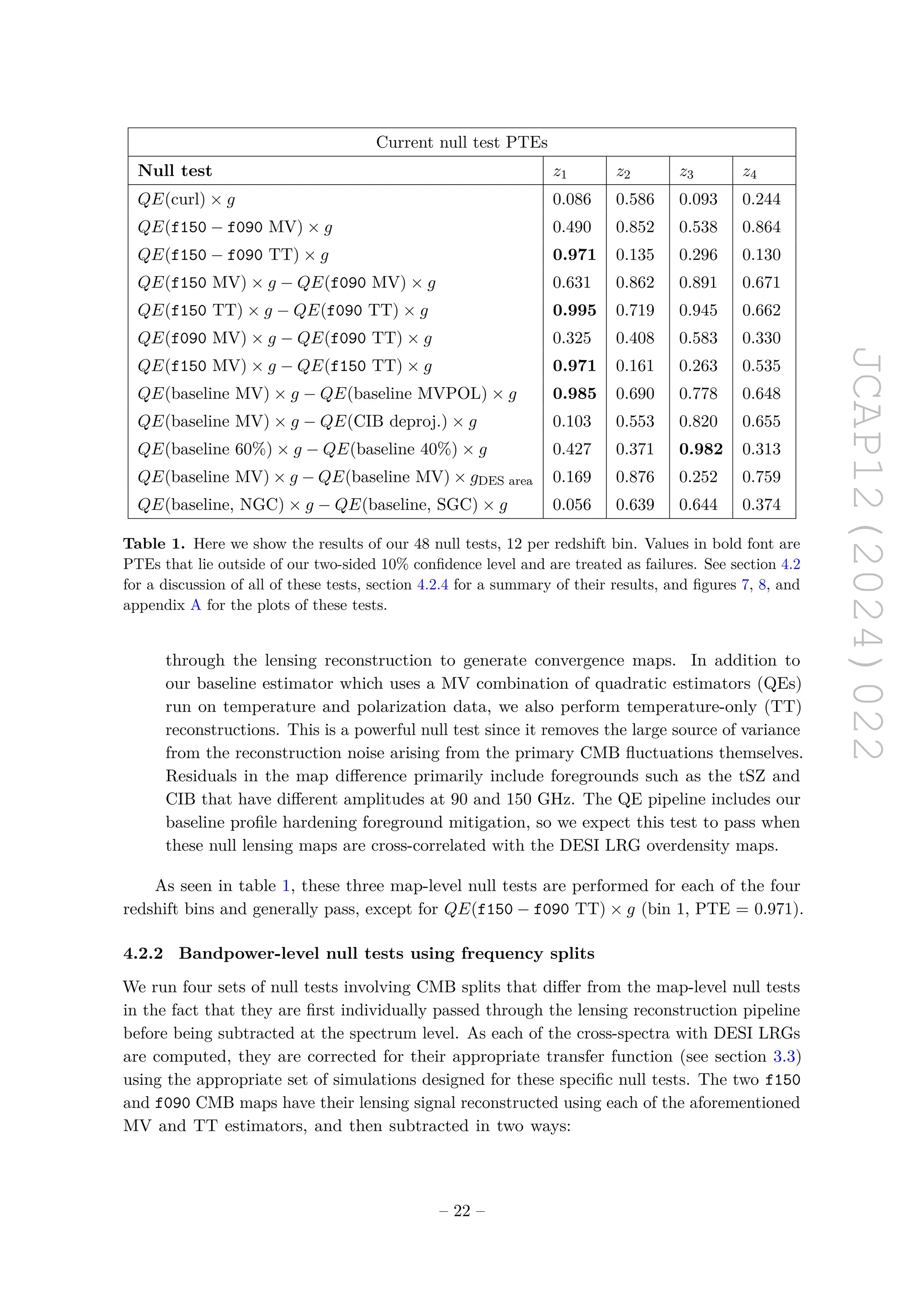
galaxy maps. As shown in table 1, all four galaxy redshift bins have a null correlation
with our confidence levels, and the results are shown in figure 7.
2. The other two map-level null tests involve a subtraction of CMB maps created by ACT
DR6 with the two frequency bands, f150 and f090. The CMB maps measured in
these two bands are subtracted to remove the lensed CMB signal, and then passed
– 21 –](https://image.slidesharecdn.com/kim2024j-250202225338-b52a3653/75/The-Atacama-Cosmology-Telescope-DR6-and-DESI-structure-formation-over-cosmic-time-with-a-measurement-of-the-cross-correlation-of-CMB-lensing-and-luminous-red-galaxies-23-2048.jpg)
![JCAP12(2024)022
• Different frequency, same QE — this is the bandpower-level version of the frequency
split map-level null tests that ensures that there is no excess signal that is present in
one CMB frequency’s cross-correlation with the galaxies with respect to the other CMB
frequency.
• Same frequency, different QE — this now checks at the bandpower level if there is
excess signal present in a galaxy cross-correlation with the MV estimator compared to
the TT estimator, and vice versa.
These 16 tests lead to 14 passes and 2 failures: QE(f150 TT) × g − QE(f090 TT) × g (bin 1,
PTE = 0.995) and QE(f150 MV) × g − QE(f150 TT) × g (bin 1 = 0.971). We have assessed
whether these high PTE failures are due to mis-estimation of the covariance by comparing
with an analytic version. A manipulation of the Gaussian covariance expression allows us to
estimate the covariance of the spectrum-level difference as the following:
Cov [Cκ1g
L − Cκ2g
L , Cκ1g
L − Cκ2g
L ] = Cov
h
C
(∆κ)g
L , C
(∆κ)g
L
i
{∆κ ≡ κ1 − κ2}
=
1
∆L(2L + 1)
×
1
fsky
×
C∆κ∆κ
L + N∆κ∆κ
L
× (Cgg
L + Ngg
L )
where ∆L is the difference in the binned centers of two consecutive bandpowers. This result
allows us to cross-check our Monte Carlo simulation-based covariance and confirm that the
errors on our bandpowers are in good agreement — we attribute these marginal failures
to statistical fluctuations.
4.2.3 Bandpower-level null tests using the baseline lensing map
The remaining null tests are now computed using the baseline MV-reconstructed lensing map,
and comparing its cross-correlation with the galaxy map to those using different variants
of the lensing product, by subtracting their respective cross-correlation bandpowers. This
includes the following:
• Minimum variance with polarization only. This is the lensing reconstruction run
using the minimum variance polarization (MVPOL) estimator, which uses a minimum
variance combination of the EE and EB quadratic estimator reconstructions. The
polarization-only map is expected to be more robust against foreground contamination
at the cost of significant degradation in signal-to-noise. The results of this null test are
shown in figure 8.
• CIB deprojected. This is an MV lensing reconstruction using a symmetrized quadratic
estimator [84, 95] in which the CIB is explicitly deprojected through a harmonic internal
linear combination (ILC) run that includes higher frequency Planck maps [65], as an
alternative to profile hardening. This specific reconstruction uses a slightly different
lensing mask that removes a few extra patches with excess Galactic dust contamination.
This null test checks if there may have been CIB contamination in our baseline map
and generally explores the robustness of our foreground mitigation.
• Conservative lensing mask. This is an MV lensing reconstruction run on a strict
subset of the baseline lensing analysis mask (which is labeled GAL060) that covers
– 23 –](https://image.slidesharecdn.com/kim2024j-250202225338-b52a3653/75/The-Atacama-Cosmology-Telescope-DR6-and-DESI-structure-formation-over-cosmic-time-with-a-measurement-of-the-cross-correlation-of-CMB-lensing-and-luminous-red-galaxies-25-2048.jpg)
![JCAP12(2024)022
0 200 400 600 800 1000
L
−1.0
−0.5
0.0
0.5
1.0
(C
κg
L,MV
−
C
κg
L,MVPOL
)
/
C
κg
L,th
Bin 1 | χ2
= 1.87, PTE = 0.98
Bin 2 | χ2
= 5.61, PTE = 0.69
Bin 3 | χ2
= 4.80, PTE = 0.78
Bin 4 | χ2
= 5.99, PTE = 0.65
0.0 0.2 0.4 0.6 0.8 1.0
PTEs
0
1
2
3
4
5
6
7
8
Counts
Figure 8. Left: the bandpower spectrum-level null test between the baseline MV reconstruction
for Cκg
L and baseline MVPOL reconstruction for Cκg
L , of which z-bin 1 “fails” due to an excessive
PTE. Right: a histogram of the PTE distribution of the 48 null tests run for this analysis, showing its
relative uniformity as well as assurance that null test failures are not systematically driven towards
high or low PTE values specifically.
approximately 40% of the full sky (GAL040) and masks out additional regions with
potential Galactic contamination. This null test checks if the baseline cross-correlation
result is free of Galactic dust contamination.
• DES footprint mask. This is an MV lensing reconstruction run with the GAL060
lensing analysis mask, but the cross-correlation is run with a more restrictive, subset
galaxy mask that only contains the active observing footprint of DES imaging data.
As described in [51], this null test checks if there is a systematic offset in the cross-
correlation within the DES sub-region only, where the imaging data is deeper and
the galaxy selection inside and outside of the sub-region can be non-trivially and
systematically different.
• NGC vs SGC. This is an MV lensing reconstruction run with the GAL060 lensing
analysis mask, but the cross-correlation is run with the intersection of the Galaxy mask
and masks that cover the North and South Galactic Caps (NGC, SGC). This null
test checks if there is an extra signal or systematic in one of the Galactic hemispheres
compared to the other.
We see 2 failures from this set of tests, QE(baseline MV)×g−QE(baseline MVPOL)×g (bin
1, PTE = 0.985) and QE(baseline 60%) × g − QE(baseline 40%) × g (bin 3, PTE = 0.982).
4.2.4 Null test summary
Again, we expect about 10% of uncorrelated null tests to fail due to statistical fluctuations
for our twelve sets of null tests run on all four galaxy redshift bins. Out of these total 48
runs, we report 5 total failures, shown in bold in table 1. Based on these results, we are
– 24 –](https://image.slidesharecdn.com/kim2024j-250202225338-b52a3653/75/The-Atacama-Cosmology-Telescope-DR6-and-DESI-structure-formation-over-cosmic-time-with-a-measurement-of-the-cross-correlation-of-CMB-lensing-and-luminous-red-galaxies-26-2048.jpg)
![JCAP12(2024)022
confident that systematics do not contribute significantly to the measurement and attribute
the null test failures to statistical fluctuations, noting also the following:
• Some of the null tests are correlated, either due to the usage of the same galaxy redshift
bin (Bin 1 has 4 of the 5 failures) or between the different products used for different
null tests (QE(f150 TT), for example, is involved in three separate failures). This
also implies that the number of uncorrelated null test failures should be appropriately
compared to the total number of uncorrelated null tests, which are both difficult to
exactly compute. However, at face value, the failure rate of uncorrelated null tests should
not significantly exceed the 10.4% value we find with our set of 5 failures out of 48 tests.
• All of the null test “failures” are due to PTEs higher than 0.95. This suggests the
following: first, these are not strictly failures in which we believe that the null test
shows a statistically significant deviation from null; second, the simulation-based error
levels for the null tests may be overestimated. To address this, the errors for all failures
were cross-checked to be in agreement between the simulation-based covariance and an
analytic Gaussian covariance. This also confirms that the non-Gaussian contributions
from lensing reconstruction that are observed in the simulations but not in the analytic
covariance are relatively small, and the mode-coupling effect is treated no differently
when using the analytic expression or the Gaussian sims.
• The distribution of PTEs is approximately uniform as expected, shown in figure 8. This
supports the idea that our PTEs are not collectively skewed towards zero or one due
to a systematic across various null tests.
In addition to these null test results, [51] confirms with parameter-level tests that by using
linear theory modeling choices and scale cuts, S8 is fully consistent with our baseline ACT-only
constraint when using variations of the ACT DR6 lensing map such as the CIB-deprojected
reconstruction, the single-frequency CMB splits, and others.
5 Cosmological constraints and analysis
Abiding by our blinding policy described in section 5.1 and confirming that parameter-level
tests (section 5.5) are acceptably passed, we perform a likelihood-based inference that uses
a theory model (section 5.2), set of priors (section 5.3), and a likelihood (section 5.4) to
estimate a constraint on S×
8 . We briefly summarize the relevant methodology in this section
and leave details to the companion paper [51].
5.1 Blinding policy
To mitigate the influence of confirmation bias, we adopt a blinding policy which prohibits
galaxy-CMB lensing cross-spectrum comparisons between ACT DR6 and Planck PR4 as well
as comparisons of both results to fiducial theory. Our blinding policy consisted of two stages:
1. Blinding at the spectrum level, during which we specifically ensured that our cross-
correlation bandpowers were never compared to theory predictions
– 25 –](https://image.slidesharecdn.com/kim2024j-250202225338-b52a3653/75/The-Atacama-Cosmology-Telescope-DR6-and-DESI-structure-formation-over-cosmic-time-with-a-measurement-of-the-cross-correlation-of-CMB-lensing-and-luminous-red-galaxies-27-2048.jpg)
![JCAP12(2024)022
2. Blinding at the parameter level, during which we specifically ensured that we did not look
at any constraints on cosmological parameters that used our unblinded cross-correlation
bandpowers
for which we only considered unblinding parameters after we had already unblinded our
bandpowers. Before unblinding our power spectra, we ensure the following:
• The pipeline is able to reproduce results of the cross-correlation between Planck PR3
lensing and DESI LRGs [50] as well as the galaxy auto-spectrum of the DESI LRGs.
• The pipeline is able to recover a fiducial prediction for the galaxy-CMB lensing cross-
spectrum as well as the galaxy auto-spectrum from correlated Gaussian simulations.
• The measurement is not contaminated significantly by Galactic and extragalactic
foregrounds, tested by populating a DESI LRG-like HOD in the Websky simulations and
observing a null cross-correlation signal with a foregrounds-only lensing reconstruction.
• The measurement is not contaminated significantly by other systematics, tested by
running a null test suite across different combinations of CMB and galaxy maps and
ensuring that at a two-sided 10% rejection level of the null hypothesis, no more than
the statistically expected number of null tests fail.
• The pipeline is able to recover input fiducial cosmological parameters using noiseless,
binned theory data vectors and the analysis covariance matrix, likelihood, priors, and
convergence criterion to good precision (summary in section 5.5, details in section 5.4
in [51]).
• The pipeline is able to recover input fiducial cosmological parameters using the Buzzard
simulations [96], for which [51] models LRG-like halos and CMB lensing to compute
a noisy cross-correlation data vector (summary in section 5.5, details in section 5.5
in [51]).
Before unblinding our constraints, we ensure the following:
• The cross-correlation measurement bandpowers between Planck PR4 and DESI LRGs
are not statistically discrepant from the bandpowers computed for the ACT DR6 and
DESI LRGs cross-correlation.
• The pipeline is able to then assess parameter-level consistency between blinded ACT
and Planck, HEFT and linear theory, as well as variations from our baseline analysis,
including conservative scale cuts for our multipole range (see figure 10) and additionally
masking LRGs on the ACT footprint.
Our blinding policy did allow us to use a blinded version of the ACT DR6 lensing
convergence map that contains a random multiplicative blinding factor for initial pipeline
development and early iterations of some null tests; this blinded map was used in other ACT
DR6 lensing analyses such as [40] and [30].
– 26 –](https://image.slidesharecdn.com/kim2024j-250202225338-b52a3653/75/The-Atacama-Cosmology-Telescope-DR6-and-DESI-structure-formation-over-cosmic-time-with-a-measurement-of-the-cross-correlation-of-CMB-lensing-and-luminous-red-galaxies-28-2048.jpg)
![JCAP12(2024)022
5.2 Theory model
We briefly summarize here our theory model, with further details found in our companion
paper [51]. We use hybrid effective field theory ([97]) to model predictions for theory spectra,
which uses a combination of the Lagrangian perturbation theory (LPT) prediction + the
Aemulus-ν simulations [98] to model the matter density field composed of both cold dark
matter and baryons. The usage of HEFT also motivates our scale cuts, as [99] cites sub-
percent accuracy for LRG-like halo clustering and halo-matter power spectra fitting for
k ≈ 0.6 h / Mpc, allowing us to probe smaller scales than what was used in [50].
HEFT allows us to parameterize cosmological power spectra as a linear combination of
the CDM + baryon power spectrum Pcb(k) and various intermediate component-basis spectra
Pi,j(k) that capture two-point correlations between different overdensities expressed in the
Lagrangian bias formalism. To 1-loop or second order, this linear combination is expressed
using a set of Lagrangian bias parameters bi for i = 1, 2, s that quantify the contribution of
the CDM + baryon overdensity fields δcb, δ2
cb, and the tidal shear field scb respectively. As
highlighted in [51], we also use counterterms α to capture interactions with the derivative
field ∇2δcb and other small-scale stochastic components. Using these bias parameters that are
independently defined and varied per redshift bin along with cosmological parameters as inputs,
predictions for the intermediate power spectra are computed efficiently by an emulator trained
on the Aemulus-ν simulations [98] which model, and then Limber integrated over the line-of-
sight to obtain predictions for the observables Cgg
L and Cκg
L . As the theory power spectrum
depends linearly on the counterterms for the galaxy auto-spectrum and the cross-spectrum
with matter as well as the shot noise SN, we can assume a Gaussian prior for these linear
parameters and analytically marginalize our likelihood with respect to them. Further details
of the marginalization procedure, and its implementation in our likelihood can be seen in [51].
5.3 Cosmological parameterization and priors
We show our priors and parameterization in table 2. To constrain the amplitude of structure,
we sample over log(1010As) and Ωch2. We fix ns and Ωbh2 to a value preferred by Planck CMB
measurements, the sum of neutrino masses
P
mν to the minimal value allowed by neutrino
oscillation experiments and Ωmh3 to a value informed by the precisely measured angular
size of the sound horizon from Planck CMB measurements.
For the HEFT model, we put priors on analytically marginalized parameters (αa for
the auto counterterm, ϵ as a parameterization of the cross counterterm, and Ngg
L for the
shot noise), the Lagrangian bias parameters b1, b2, and bs (up to second or 1-loop order),
and the magnification bias µ. We put relatively uninformative priors on all of these HEFT
parameters except for bs and ϵ, where the former is found to share a strong degeneracy
with b2 and the latter is chosen to appropriately represent the size of small-scale effects
we expect from baryonic feedback [32] and our usage of the Aemulus-ν simulations. These
are discussed in further detail in [51].
– 27 –](https://image.slidesharecdn.com/kim2024j-250202225338-b52a3653/75/The-Atacama-Cosmology-Telescope-DR6-and-DESI-structure-formation-over-cosmic-time-with-a-measurement-of-the-cross-correlation-of-CMB-lensing-and-luminous-red-galaxies-29-2048.jpg)
![JCAP12(2024)022
Parameter Prior
Fixed parameters
ns 0.9649
Ωbh2 0.02236
Ωmh3 0.09633
P
mν 0.06 eV
Cosmological parameters
log(1010As) U(2, 4)
Ωch2 U(0.08, 0.16)
Analytically marginalized parameters
αa N(0, 50)
ϵ N(0, 2)
Ngg
L 10−6 N(4.07 | 2.25 | 2.05 | 2.25, 0.3 × 4.07 | 2.25 | 2.05 | 2.25)
Nuisance parameters
b1 U(0, 3)
b2 U(−5, 5)
bs N(0, 1)
µi N(0.972 | 1.044 | 0.974 | 0.988, 0.1)
Table 2. Parameters and priors used in this work and [51]. Uniform priors from x1 to x2 are denoted
with U(x1, x2) and Gaussian priors with mean µ and standard deviation σ are shown as N(µ, σ).
Nuisance parameters b1, b2, bs are all bias parameters for the HEFT theory model; counterterms are
represented with αa and ϵ; and µi is the magnification bias for galaxy redshift bin zi. Only the shot
noise spectrum Ngg
L and magnification bias µi have redshift bin-dependent priors, with µ and σ shown
respectively for bins 1, 2, 3, and 4.
5.4 Parameter inference
We adopt a Gaussian likelihood, taking the form:
−2 ln L ∝
Ĉκg
L − Cκg
L (θ)
Ĉgg
L − Cgg
L (θ)
T
Cov(Cκg
L , Cκg
L′ ) Cov(Cκg
L , Cgg
L′ )
Cov(Cgg
L , Cκg
L′ ) Cov(Cgg
L , Cgg
L′ )
−1
Ĉκg
L′ − Cκg
L′ (θ)
Ĉgg
L′ − Cgg
L′ (θ)
(5.1)
where ĈAB
L for AB ∈ {κg, gg} represents a power spectrum measurement, CAB
L (θ) represents
the prediction from the HEFT matter and galaxy power spectra using cosmological parameters
θ, and the covariance blocks Cov
CAB
L , CCD
L′
are computed as described in section 3.4.
The cosmological parameter space was sampled using the Markov Chain Monte Carlo
(MCMC) method with the Cobaya framework [103, 104], and best-fit values were obtained
by using the minimize sampler built in Cobaya. The MCMC chains were sampled using the
likelihood from section 5.1 until a Gelman-Rubin convergence criterion [105] of R − 1 0.01
was reached. The first 30% of the chains are removed as burn-in chains before the contours
are visualized and analyzed using GetDist [106].
– 28 –](https://image.slidesharecdn.com/kim2024j-250202225338-b52a3653/75/The-Atacama-Cosmology-Telescope-DR6-and-DESI-structure-formation-over-cosmic-time-with-a-measurement-of-the-cross-correlation-of-CMB-lensing-and-luminous-red-galaxies-30-2048.jpg)
![JCAP12(2024)022
0.4 0.5 0.6 0.7 0.8 0.9 1.0
z
0.45
0.50
0.55
0.60
0.65
0.70
0.75
S
×
8
(z)
=
σ
8
(z)
(Ω
0
m
/
0.3)
0.4
Planck PR3 (Planck+20)
Planck PR4 (Tristram+23)
Planck PR4 (Rosenberg+22)
Planck PR4 only
ACT DR6 only
Best-fits
Bin 1 (ACT+Planck)
Bin 2 (ACT+Planck)
Bin 3 (ACT+Planck)
Bin 4 (ACT+Planck)
0.5 0.6 0.7 0.8 0.9 1.0 1.1 1.2
z
0.45
0.50
0.55
0.60
0.65
0.70
0.75
S
×
8
(z)
=
σ
8
(z)
(Ω
0
m
/
0.3)
0.4
Planck PR4 CMB aniso. (Rosenberg et al. 2022)
ACT+Planck CMB lensing x DESI LRGs (this work)
ACT+Planck CMB lensing x unWISE (Farren et al. 2023)
Figure 9. Left: S×
8 (z) shown for our four redshift bins with the Planck PR4 measurement, ACT
DR6 measurement, and the joint ACT + Planck fit. We note the means are consistent with the
best-fit points shown as open markers, and that these means are consistently low compared to the
Planck PR4 CMB prediction in concordance with the baseline joint-redshift constraint. The theory
predictions computed using CAMB ([100–102]) with the Planck cosmological parameters are shown in
dashed lines. Right: showing same joint ACT + Planck fits as left, but we also plot the unWISE
cross-correlation result with Planck PR4, ACT DR6, and their joint fit from [40], which sees better
agreement with the Planck PR3 CMB at lower redshifts.
The MCMC sampling is also run on each redshift bin independently, where only the
nuisance parameters for each bin is sampled along with the appropriate cosmological parame-
ters. This information from the best-fit cosmologies can be used to understand the redshift
dependence of structure growth, as we can compute and plot a redshift-dependent S×
8 (z)9
for each of our redshift bin means, defined as the following:
S×
8 (z) = σ8(z)
Ωm(z = 0)
0.3
0.4
(5.2)
which is a rescaling of S×
8 (z = 0) measured from each redshift bin, computed by assuming
the Planck PR3 fiducial cosmology [1] to evaluate the matter power spectrum and the linear
growth factor D(z) using CAMB ([100–102]) for both Ωm(z = 0) and σ8(z):
σ8(z) = D(z) σPR3
8 (z = 0). (5.3)
This leads to the implication that if our parameter of structure formation at the present-day
is in agreement with Planck, our structure growth amplitude should scale using this function
of redshift with the same behavior shown by Planck. These rescaled, redshift-dependent
constraints are shown in figure 9.
5.5 Parameter recovery tests
To ensure we are robust to biases from “prior volume” effects, where the posterior mean is
found to deviate from the maximum a posteriori value due to the influence of a number of
9
S×
8 (z) constraints are not to be confused with the redshift-independent constraints denoted in this paper
as S×
8 which are defined at z = 0.
– 29 –](https://image.slidesharecdn.com/kim2024j-250202225338-b52a3653/75/The-Atacama-Cosmology-Telescope-DR6-and-DESI-structure-formation-over-cosmic-time-with-a-measurement-of-the-cross-correlation-of-CMB-lensing-and-luminous-red-galaxies-31-2048.jpg)
![JCAP12(2024)022
prior-dominated parameters, we perform parameter recovery tests in which we attempt to
recover exactly known input cosmological parameters using noiseless theory spectra computed
using those same exact parameters.
To do this, we bin a set of noiseless theory spectra in the same way as our measurement’s
data bandpowers are binned (see section 3.1), and pass that into our MCMC sampler as the
data vector. We use our joint hybrid covariance matrix described in section 3.4 that contains
information from the ACT DR6 x DESI LRG cross-correlation, the Planck PR4 x DESI LRG
cross-correlation, and the DESI LRG auto-correlation spectra. This parameter recovery test
also allows us to measure the Ωm dependence on this paper’s headline result, which is the
combination of σ8 and Ωm with the lowest relative error — we compute this to be:
S×
8 = σ8
Ωm
0.3
0.4
(5.4)
Using the Buzzard simulations and their associated cosmological parameters as inputs
to generate noiseless theory spectra, the parameter recovery test allows us to recover S×
8 to
within less than 0.1 σ from the input value (considering both the posterior mean as well as
the best-fit) for the baseline joint Planck + ACT analysis when combining all redshift bins
and under 0.4 σ for different combinations of Planck and ACT with individual redshift bins.
This test is not to be confused with a similar systematics test of fitting to the Buzzard
simulations’ data vector, which is noisy and computed using a simulated CMB lensing
convergence field intrinsic to the simulation suite. This test confirms the robustness of the
theory model and also acts as a robustness check for the appropriate bandpower window
functions, pixel window function, analysis covariance matrices, and choice of priors. Further
details of this test and adequate recoveries of S8 and σ8 with and without a BAO prior
are described in section 5.5 in [51], where S×
8 is recovered and constrained to a posterior
mean and best-fit value less than 0.5 σ from truth for all combinations of redshift bins
and covariance matrices.
5.6 Results
Combining the posterior information from the ACT DR6 x DESI LRG cross-correlation
power spectrum and DESI LRG auto-correlation power spectrum, we have (with best-fit
values in brackets):
S×
8 [DR6] = 0.792+0.024
−0.028 [0.797] (5.5)
The combination of the Planck PR4 x DESI LRG cross-correlation power spectrum and
the DESI LRG auto-correlation power spectrum gives us a slightly tighter constraint albeit
a lower mean:
S×
8 [PR4] = 0.766 ± 0.022 [0.769] (5.6)
Our baseline results use the combination of ACT and Planck cross-correlations with DESI,
which yields this analysis’s strongest constraint at 2.7%:
S×
8 ≡ σ8
Ωm
0.3
0.4
= 0.776+0.019
−0.021 [0.776] (5.7)
– 30 –](https://image.slidesharecdn.com/kim2024j-250202225338-b52a3653/75/The-Atacama-Cosmology-Telescope-DR6-and-DESI-structure-formation-over-cosmic-time-with-a-measurement-of-the-cross-correlation-of-CMB-lensing-and-luminous-red-galaxies-32-2048.jpg)
![JCAP12(2024)022
kmax Lmax (z1 → z4) DR6 PR4 DR6 + PR4 S×
8 % constraint
0.1 h/Mpc 124, 124, 178, 178 22 23 31 3.3%
0.15 h/Mpc 178, 178, 243, 317 28 29 38 2.9%
0.2 h/Mpc 243, 317, 317, 401 31 33 43 2.7%
Baseline (0.5 h/Mpc) 600, 600, 600, 600 38 39 50 2.7%
Table 3. This table shows the signal-to-noise ratio (computed as
p
χ2, see appendix B) of the Cκg
L
measurement with ACT DR6 lensing, Planck PR4 lensing, and the joint ACT + Planck analysis;
the corresponding strongest percentage constraint of S×
8 inferred from their respective posteriors are
shown in the right-most column, each shown with its dependence on the maximum scale wavenumber,
kmax. For each redshift bin, we relate this kmax to the maximum angular multipole Lmax using the
comoving distance corresponding to the peak of the redshift distribution, and use Lmax to determine
the scales in the covariance matrix and fiducial theory bandpowers used to compute χ2
. The results
show us also how much improvement we gain in our fractional constraint and SNR by using HEFT
and smaller scales compared to a linear theory-like model (first three entries).
a result that is approximately 2.1σ10 lower (1.2σ lower for ACT only) than the Planck PR4
prediction of:
S×
8 = 0.826 ± 0.012 (5.8)
from the primary CMB anisotropies (2.2σ lower than Planck PR3), while being in general
agreement with the late-time galaxy lensing constraints. In all three cases we see no significant
tension between the best-fit values and the posterior means, showing that we are not affected
by prior volume effects on S×
8 . A feature of these results is that, as seen in figure 10, the
constraint from using only the lowest redshift bin is more than 0.5σ low from the baseline
constraint mean, an effect that was similarly observed in [50] but to a greater extent than our
analysis’s findings; this effect is not specific to the Planck-only cross-correlation as the ACT-
only constraint for this redshift bin presents a similar discrepancy from the Planck primary
CMB. This lowest redshift bin is the least constraining and features the largest error bars of
the four redshift bins. We proceeded to run a joint constraint while excluding this lowest
redshift bin, which pushes our S×
8 mean to a slightly higher value (S×
8 = 0.785+0.021
−0.023) but
not high enough to be in tension ( 0.3σ) with our baseline result. We also run a set of
varied constraints where the maximum multipole scale cuts are more conservative and reflect
the maximum k and L scale cuts shown in figure 3; these results are still consistent with
our baseline constraint on S×
8 , showing that our analysis is robust to different scale cuts.
Further details on a thorough test of our consistency with a linear theory model and a “model
independent” approach can be seen in our companion paper [51].
We show S×
8 (z) for each of our 4 redshift bins in figure 9 by rescaling the ACT +
Planck S×
8 means and errors from redshift zero to their effective redshifts (see table 1 in [51]);
10
Here and throughout the paper, we define a difference or discrepancy between measurement µ1 ± σ1 and
measurement µ2 ± σ2 as (µ1 − µ2)/
p
σ2
1 + σ2
2. For a posterior constraint with asymmetric error bars µ+x
−y, we
compute and quote differences using the standard deviation of the samples used to construct the posterior.
– 31 –](https://image.slidesharecdn.com/kim2024j-250202225338-b52a3653/75/The-Atacama-Cosmology-Telescope-DR6-and-DESI-structure-formation-over-cosmic-time-with-a-measurement-of-the-cross-correlation-of-CMB-lensing-and-luminous-red-galaxies-33-2048.jpg)
![JCAP12(2024)022
0.65 0.70 0.75 0.80 0.85
S×
8 ≡ σ8(Ωm/0.3)0.4
ACT DR6 + Planck PR4 x DESI
ACT DR6 x DESI LRGs
Planck PR4 x DESI LRGs
Joint, z1 only
Joint, z2 only
Joint, z3 only
Joint, z4 only
Joint, no z1
Joint, conservative kmax = 0.1 h/Mpc
Joint, conservative kmax = 0.15 h/Mpc
Joint, conservative kmax = 0.2 h/Mpc
Figure 10. We show S×
8 constraints using different analysis variations and demonstrate their
consistency with the baseline constraints, shown in yellow for ACT + Planck, ACT only, and
Planck only respectively. The red points show the joint ACT DR6 and Planck PR4 constraints when
fit to each redshift bin independently; seeing that the mean of the lowest redshift bin lies outside the
1σ range of our baseline constraint (a feature of this redshift bin we also see with the ACT-only and
Planck-only cross-correlations in figure 9), we verify that the combination of the other 3 redshift bins
(shown in purple) is consistent with our baseline mean. The blue points show our analysis carried
out with the conservative scale cuts shown in table 3. For reference, we also show a green band
representing the constraint from the Planck PR4 primary CMB anisotropies [2].
curly bracketed values represent the Planck PR4 [2] primary CMB prediction of S×
8 (z):
S×
8 (z = 0.470) = 0.572+0.032
−0.048 {0.641}
S×
8 (z = 0.625) = 0.560+0.025
−0.031 {0.594}
S×
8 (z = 0.785) = 0.525+0.021
−0.025 {0.550}
S×
8 (z = 0.914) = 0.498 ± 0.019 {0.518}
and note that the first redshift bin as we found previously shows the lowest mean compared
to the primary CMB prediction. As demonstrated in the companion paper [51], these S×
8 (z)
values are correlated with each other by approximately 0–30%, with higher correlations
found between redshift bins 3 and 4 (that we also observe in figure 6); an optimal linear
combination of the S×
8 (z) constraints weighted by their respective correlations recovers the
baseline joint constraint to 0.1σ, confirming our lower value with Planck PR3 at the
2.2 σ significance level.
– 32 –](https://image.slidesharecdn.com/kim2024j-250202225338-b52a3653/75/The-Atacama-Cosmology-Telescope-DR6-and-DESI-structure-formation-over-cosmic-time-with-a-measurement-of-the-cross-correlation-of-CMB-lensing-and-luminous-red-galaxies-34-2048.jpg)
![JCAP12(2024)022
0.6 0.7 0.8 0.9
S×
8 ≡ σ8(Ωm/0.3)0.4
Rosenberg et al. 2022
Madhavacheril et al. 2023
Carron et al. 2022
Madhavacheril et al. 2023
Bianchini et al. 2020
Farren et al. 2023
Marques et al. 2023
Chang et al. 2022
Secco et al. 2021,
Amon et al. 2021
Longley et al. 2022,
Asgari et al. 2020
Dalal et al. 2023
Li et al. 2023
Planck PR4 CMB aniso.
Primary CMB
ACT DR6 CMB lensing + BAO
CMB lensing
Planck PR4 CMB lensing + BAO
ACT+Planck CMB lensing + BAO
SPTPol CMB lensing + BAO
ACT DR6 + Planck PR4 x DESI LRGs
This work
ACT DR6 x DESI LRGs
Planck PR4 x DESI LRGs
ACT DR6 + Planck PR4 x unWISE
CMB lensing
ACT DR4 x DES MagLim
cross-corr.
DES-Y3 x SPT + Planck PR3
DES-Y3 galaxy lensing + BAO
Galaxy weak
KiDS-1000 galaxy lensing + BAO
lensing
HSC-Y3 galaxy lensing (Fourier) + BAO
HSC-Y3 galaxy lensing (Real) + BAO
Figure 11. We show our constraint on S×
8 with the ACT DR6 cross-correlation, Planck PR4 cross-
correlation, and the joint ACT and Planck analysis in yellow. We find that we are not in substantial
disagreement with constraints from the primary CMB (in green, [2]), CMB lensing power spectrum
(in red, [28, 29, 107]), and from galaxy weak lensing (in blue, [19, 20, 108–111]). We have various
levels of agreement with different galaxy-CMB lensing cross-correlations (in purple, [37, 39, 40, 50])
and lower redshift tracers (such as DES MagLim [37], unWISE Green, Blue [40]).
6 Summary and discussion
Through a harmonic-space tomographic cross-correlation between state-of-the-art CMB
lensing maps from Planck and ACT with DESI LRGs, we have obtained a 2.7% constraint
on the parameter combination S×
8 ≡ σ8(Ωm/0.3)0.4 characterizing the amplitude of matter
fluctuations. As seen in figure 11, our ACT-only constraint of S×
8 = 0.792+0.024
−0.028 and our joint
ACT + Planck constraint of S×
8 = 0.776+0.019
−0.021 are roughly consistent both with the Planck PR4
primary CMB anisotropy prediction (our ACT-only and joint constraints are lower by 1.2σ
and 2.1σ respectively) as well as with other large scale structure (LSS) constraints (which
generally come lower than the Planck prediction by 1 − 2.5σ). An open question is whether
the mild discrepancy of several of these LSS probes is driven by new physics, unaccounted
astrophysical processes (e.g., baryonic feedback), systematics, or statistical fluctuations. Since
every probe has sensitivity to different scales and redshifts, high-precision cross-correlations
such as from this work bring us closer to clarifying the origin of these discrepancies.
This cross-correlation result computed for four redshift bins is robust and verified to be not
significantly biased by extragalactic or Galactic foregrounds as well as other systematics. We
demonstrate this using the LRG-like HOD cross-correlation test with the Websky foregrounds-
– 33 –](https://image.slidesharecdn.com/kim2024j-250202225338-b52a3653/75/The-Atacama-Cosmology-Telescope-DR6-and-DESI-structure-formation-over-cosmic-time-with-a-measurement-of-the-cross-correlation-of-CMB-lensing-and-luminous-red-galaxies-35-2048.jpg)
![JCAP12(2024)022
only reconstruction along with our comprehensive suite of 48 null tests using a variety of
ACT DR6 lensing products in which we see no significant spurious correlations with expected
null signals. We follow a blinding procedure to avoid the influence of confirmation bias, and
ensure that the analysis design choices including the HEFT theory modeling, multipole scale
cuts, “hybrid” covariance matrix, and likelihood / prior parameterization are devised and
fixed before comparing and fitting our theory model to the unblinded data.
Generally, constraints from the CMB lensing auto-spectrum (which probe predominantly
higher redshifts z = 1 − 2 and linear scales k 0.2 Mpc−1
) show excellent agreement with the
Planck CMB prediction. At the same time, cross-correlations of CMB lensing with unWISE
(probing z ∼ 0.6 and z ∼ 1.1) are also consistent with Planck. We have explored the redshift
dependence of our S×
8 constraint by separately constraining this parameter for each redshift
bin. While all bins remain nominally consistent with Planck, the lowest redshift bin shows the
largest difference in the mean S×
8 value; an analysis that excludes this redshift bin is consistent
with Planck at 1.6σ. This may be an indication of new physics (e.g., modified gravity), a
systematic that affects lower redshifts more, or a statistical fluctuation, though no strong
conclusion can be drawn given the uncertainty on our lowest redshift bin. Future CMB lensing
cross-correlations with the DESI Legacy Imaging galaxies [112, 113], DESI Bright Galaxy
Sample (BGS) and other lower redshift samples will be key to assessing this conclusively.
These cross-correlations will also be significantly improved in precision with future CMB
lensing surveys such as the Simons Observatory (SO, [114]), CMB-Stage 4 (CMB-S4, [115]),
and CMB-HD ([116]), allowing for a path to disentangling possible discrepancies between
early-time and late-time observations of structure formation.
Acknowledgments
We would like to thank Bruce Partridge for helpful discussions in preparing this manuscript.
JK acknowledges support from NSF grants AST-2307727 and AST-2153201. NS is
supported by the Office of Science Graduate Student Research (SCGSR) program administered
by the Oak Ridge Institute for Science and Education for the DOE under contract number
DE-SC0014664. MM acknowledges support from NSF grants AST-2307727 and AST-2153201
and NASA grant 21-ATP21-0145. SF is supported by Lawrence Berkeley National Laboratory
and the Director, Office of Science, Office of High Energy Physics of the U.S. Department of
Energy under Contract No. DE-AC02-05CH11231. GSF acknowledges support through the
Isaac Newton Studentship and the Helen Stone Scholarship at the University of Cambridge.
GSF and BDS acknowledge support from the European Research Council (ERC) under
the European Union’s Horizon 2020 research and innovation programme (Grant agreement
No. 851274). EC acknowledges support from the European Research Council (ERC) under
the European Union’s Horizon 2020 research and innovation programme (Grant agreement
No. 849169). GAM is part of Fermi Research Alliance, LLC under Contract No. DE-
AC02-07CH11359 with the U.S. Department of Energy, Office of Science, Office of High
Energy Physics. KM acknowledges support from the National Research Foundation of
South Africa. CS acknowledges support from the Agencia Nacional de Investigación y
Desarrollo (ANID) through Basal project FB210003. OD acknowledges support from a SNSF
Eccellenza Professorial Fellowship (No. 186879). JD acknowledges support from NSF award
– 34 –](https://image.slidesharecdn.com/kim2024j-250202225338-b52a3653/75/The-Atacama-Cosmology-Telescope-DR6-and-DESI-structure-formation-over-cosmic-time-with-a-measurement-of-the-cross-correlation-of-CMB-lensing-and-luminous-red-galaxies-36-2048.jpg)
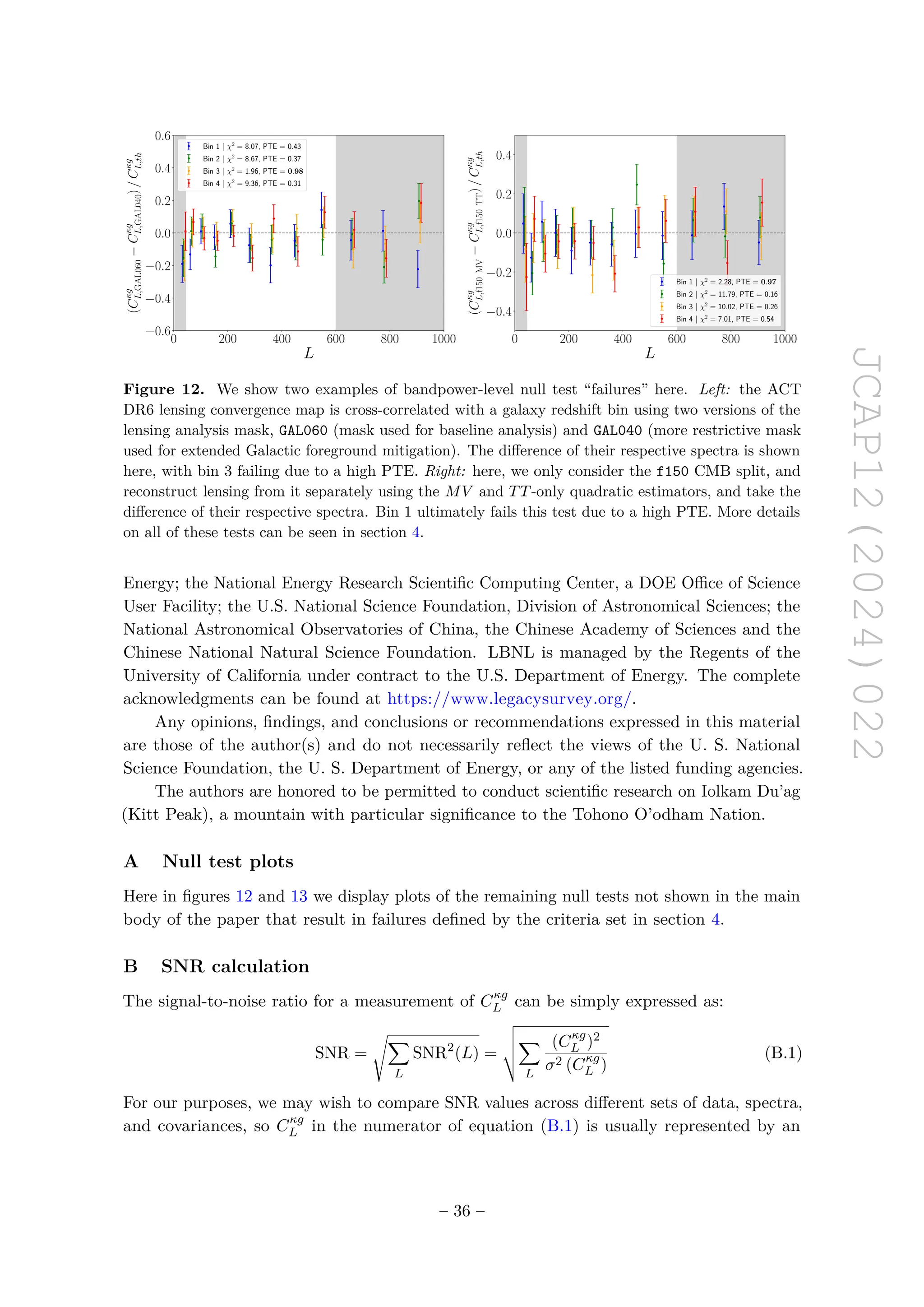
![JCAP12(2024)022
0 200 400 600 800 1000
L
−0.75
−0.50
−0.25
0.00
0.25
0.50
0.75
(C
κg
L,f150
TT
−
C
κg
L,f090
TT
)
/
C
κg
L,th
Bin 1 | χ2
= 1.37, PTE = 0.99
Bin 2 | χ2
= 5.35, PTE = 0.72
Bin 3 | χ2
= 2.82, PTE = 0.94
Bin 4 | χ2
= 5.86, PTE = 0.66
0 200 400 600 800 1000
L
−0.4
−0.2
0.0
0.2
0.4
C
QE(f150
TT,f090
TT)×g
L
/
C
κg
L,th
Bin 1 | χ2
= 2.28, PTE = 0.97
Bin 2 | χ2
= 12.37, PTE = 0.14
Bin 3 | χ2
= 9.58, PTE = 0.30
Bin 4 | χ2
= 12.51, PTE = 0.13
Figure 13. We show the results of a null test computed with the f150 CMB split and the f090 CMB
split, with different combinations passed into a TT-only CMB lensing reconstruction. The fact that
both of these tests “fail” for using the same data products for the same redshift bin (Bin 1) shows
that these outcomes are likely to be correlated. Left: the difference is computed after each CMB
split is passed into the reconstruction pipeline, with each reconstructed convergence cross-correlated
with a galaxy redshift bin and subtracted as spectra (bandpower-level). Right: the difference is
computed before passing the data product into the reconstruction pipeline, with the lensing signal
reconstructed from the map difference of the CMB splits and then cross-correlated with a galaxy
redshift bin (map-level). More details on all of these tests can be seen in section 4.
invariant fiducial theory spectrum while the σ’s may change depending on the error bars
placed on a specific measurement.
However, summing over each bandpower independently ignores correlations between
bandpowers, so one takes into account C, the covariance matrix block for d = Cκg
L , in lieu
of the latter expression:
SNR =
p
dT
· C−1 · d ≡
q
χ2(Cκg
L ) (B.2)
where the cumulative SNR for a multipole range of [Lmin, Lmax] can be expressed as:
SNR(Lmin, Lmax) =
Lmax
X
L=Lmin
Lmax
X
L′=Lmin
Cκg
L × Cov Cκg
L , Cκg
L′
−1
× Cκg
L′
1/2
(B.3)
To compute the contribution to the SNR per bandpower, we compute the following for a
given binning scheme of bin edges Li ∈ [L0 (= Lmin), L1, . . . , Lmax]:
SNR(Li, Li+1) =
q
SNR2
(Lmin, Li+1) − SNR2
(Lmin, Li) (B.4)
where the right side of this equation is computed using equation (B.3). This value is plotted
for each analysis multipole bin in figure 2 after applying an arbitrary normalization factor,
and the relative fraction of the SNR that each bandpower contributes can be calculated by
dividing the value for each bin by the baseline total SNR found in table 3.
– 37 –](https://image.slidesharecdn.com/kim2024j-250202225338-b52a3653/75/The-Atacama-Cosmology-Telescope-DR6-and-DESI-structure-formation-over-cosmic-time-with-a-measurement-of-the-cross-correlation-of-CMB-lensing-and-luminous-red-galaxies-39-2048.jpg)
![JCAP12(2024)022
References
[1] Planck collaboration, Planck 2018 results. VI. Cosmological parameters, Astron. Astrophys.
641 (2020) A6 [Erratum ibid. 652 (2021) C4] [arXiv:1807.06209] [INSPIRE].
[2] E. Rosenberg, S. Gratton and G. Efstathiou, CMB power spectra and cosmological parameters
from Planck PR4 with CamSpec, Mon. Not. Roy. Astron. Soc. 517 (2022) 4620
[arXiv:2205.10869] [INSPIRE].
[3] ACT collaboration, The Atacama Cosmology Telescope: DR4 maps and cosmological
parameters, JCAP 12 (2020) 047 [arXiv:2007.07288] [INSPIRE].
[4] SPT-3G collaboration, Measurement of the CMB temperature power spectrum and constraints
on cosmology from the SPT-3G 2018 TT, TE, and EE dataset, Phys. Rev. D 108 (2023) 023510
[arXiv:2212.05642] [INSPIRE].
[5] A. Lewis and A. Challinor, Weak gravitational lensing of the CMB, Phys. Rept. 429 (2006) 1
[astro-ph/0601594] [INSPIRE].
[6] eBOSS collaboration, The clustering of the SDSS-IV extended Baryon Oscillation
Spectroscopic Survey DR14 LRG sample: structure growth rate measurement from the
anisotropic LRG correlation function in the redshift range 0.6 z 1.0, Mon. Not. Roy.
Astron. Soc. 492 (2020) 4189 [arXiv:1909.07742] [INSPIRE].
[7] O.H.E. Philcox and M.M. Ivanov, BOSS DR12 full-shape cosmology: ΛCDM constraints from
the large-scale galaxy power spectrum and bispectrum monopole, Phys. Rev. D 105 (2022)
043517 [arXiv:2112.04515] [INSPIRE].
[8] T. Simon, P. Zhang and V. Poulin, Cosmological inference from the EFTofLSS: the eBOSS
QSO full-shape analysis, JCAP 07 (2023) 041 [arXiv:2210.14931] [INSPIRE].
[9] V. Ghirardini et al., The SRG/eROSITA all-sky survey — cosmology constraints from cluster
abundances in the western galactic hemisphere, Astron. Astrophys. 689 (2024) A298
[arXiv:2402.08458] [INSPIRE].
[10] SPT and DES collaborations, SPT clusters with DES and HST weak lensing. II. Cosmological
constraints from the abundance of massive halos, Phys. Rev. D 110 (2024) 083510
[arXiv:2401.02075] [INSPIRE].
[11] DES collaboration, The dark energy camera, Astron. J. 150 (2015) 150 [arXiv:1504.02900]
[INSPIRE].
[12] DES collaboration, Dark Energy Survey year 3 results: cosmological constraints from galaxy
clustering and weak lensing, Phys. Rev. D 105 (2022) 023520 [arXiv:2105.13549] [INSPIRE].
[13] K. Kuijken et al., Gravitational lensing analysis of the Kilo Degree Survey, Mon. Not. Roy.
Astron. Soc. 454 (2015) 3500 [arXiv:1507.00738] [INSPIRE].
[14] C. Heymans et al., KiDS-1000 cosmology: multi-probe weak gravitational lensing and
spectroscopic galaxy clustering constraints, Astron. Astrophys. 646 (2021) A140
[arXiv:2007.15632] [INSPIRE].
[15] H. Aihara et al., The Hyper Suprime-Cam SSP survey: overview and survey design, Publ.
Astron. Soc. Jap. 70 (2018) S4 [arXiv:1704.05858] [INSPIRE].
[16] S. More et al., Hyper Suprime-Cam year 3 results: measurements of clustering of SDSS-BOSS
galaxies, galaxy-galaxy lensing, and cosmic shear, Phys. Rev. D 108 (2023) 123520
[arXiv:2304.00703] [INSPIRE].
– 38 –](https://image.slidesharecdn.com/kim2024j-250202225338-b52a3653/75/The-Atacama-Cosmology-Telescope-DR6-and-DESI-structure-formation-over-cosmic-time-with-a-measurement-of-the-cross-correlation-of-CMB-lensing-and-luminous-red-galaxies-40-2048.jpg)
![JCAP12(2024)022
[17] H. Miyatake et al., Hyper Suprime-Cam Year 3 results: cosmology from galaxy clustering and
weak lensing with HSC and SDSS using the emulator based halo model, Phys. Rev. D 108
(2023) 123517 [arXiv:2304.00704] [INSPIRE].
[18] S. Sugiyama et al., Hyper Suprime-Cam Year 3 results: cosmology from galaxy clustering and
weak lensing with HSC and SDSS using the minimal bias model, Phys. Rev. D 108 (2023)
123521 [arXiv:2304.00705] [INSPIRE].
[19] R. Dalal et al., Hyper Suprime-Cam Year 3 results: cosmology from cosmic shear power spectra,
Phys. Rev. D 108 (2023) 123519 [arXiv:2304.00701] [INSPIRE].
[20] X. Li et al., Hyper Suprime-Cam Year 3 results: cosmology from cosmic shear two-point
correlation functions, Phys. Rev. D 108 (2023) 123518 [arXiv:2304.00702] [INSPIRE].
[21] C. Heymans et al., CFHTLenS: the Canada-France-Hawaii telescope lensing survey, Mon. Not.
Roy. Astron. Soc. 427 (2012) 146 [arXiv:1210.0032] [INSPIRE].
[22] Planck collaboration, Planck 2015 results. XIII. Cosmological parameters, Astron. Astrophys.
594 (2016) A13 [arXiv:1502.01589] [INSPIRE].
[23] A. Leauthaud et al., Lensing is low: cosmology, galaxy formation, or new physics?, Mon. Not.
Roy. Astron. Soc. 467 (2017) 3024 [arXiv:1611.08606] [INSPIRE].
[24] S. Joudaki et al., CFHTLenS revisited: assessing concordance with Planck including
astrophysical systematics, Mon. Not. Roy. Astron. Soc. 465 (2017) 2033 [arXiv:1601.05786]
[INSPIRE].
[25] M.M. Ivanov et al., Cosmology with the galaxy bispectrum multipoles: optimal estimation and
application to BOSS data, Phys. Rev. D 107 (2023) 083515 [arXiv:2302.04414] [INSPIRE].
[26] eBOSS collaboration, Completed SDSS-IV extended Baryon Oscillation Spectroscopic Survey:
cosmological implications from two decades of spectroscopic surveys at the Apache Point
Observatory, Phys. Rev. D 103 (2021) 083533 [arXiv:2007.08991] [INSPIRE].
[27] Kilo-Degree Survey and DES collaborations, DES Y3 + KiDS-1000: consistent cosmology
combining cosmic shear surveys, Open J. Astrophys. 6 (2023) 2305.17173 [arXiv:2305.17173]
[INSPIRE].
[28] ACT collaboration, The Atacama Cosmology Telescope: DR6 gravitational lensing map and
cosmological parameters, Astrophys. J. 962 (2024) 113 [arXiv:2304.05203] [INSPIRE].
[29] J. Carron, M. Mirmelstein and A. Lewis, CMB lensing from Planck PR4 maps, JCAP 09
(2022) 039 [arXiv:2206.07773] [INSPIRE].
[30] ACT collaboration, The Atacama Cosmology Telescope: a measurement of the DR6 CMB
lensing power spectrum and its implications for structure growth, Astrophys. J. 962 (2024) 112
[arXiv:2304.05202] [INSPIRE].
[31] SPT collaboration, Measurement of gravitational lensing of the cosmic microwave background
using SPT-3G 2018 data, Phys. Rev. D 108 (2023) 122005 [arXiv:2308.11608] [INSPIRE].
[32] A. Amon and G. Efstathiou, A non-linear solution to the S8 tension?, Mon. Not. Roy. Astron.
Soc. 516 (2022) 5355 [arXiv:2206.11794] [INSPIRE].
[33] C. Preston, A. Amon and G. Efstathiou, A non-linear solution to the S8 tension — II. Analysis
of DES year 3 cosmic shear, Mon. Not. Roy. Astron. Soc. 525 (2023) 5554 [arXiv:2305.09827]
[INSPIRE].
– 39 –](https://image.slidesharecdn.com/kim2024j-250202225338-b52a3653/75/The-Atacama-Cosmology-Telescope-DR6-and-DESI-structure-formation-over-cosmic-time-with-a-measurement-of-the-cross-correlation-of-CMB-lensing-and-luminous-red-galaxies-41-2048.jpg)
![JCAP12(2024)022
[34] K.K. Rogers et al., Ultra-light axions and the S8 tension: joint constraints from the cosmic
microwave background and galaxy clustering, JCAP 06 (2023) 023 [arXiv:2301.08361]
[INSPIRE].
[35] Atacama Cosmology Telescope collaboration, Atacama Cosmology Telescope: combined
kinematic and thermal Sunyaev-Zel’dovich measurements from BOSS CMASS and LOWZ halos,
Phys. Rev. D 103 (2021) 063513 [arXiv:2009.05557] [INSPIRE].
[36] S. Amodeo et al., Atacama Cosmology Telescope: modeling the gas thermodynamics in BOSS
CMASS galaxies from kinematic and thermal Sunyaev-Zel’dovich measurements, Phys. Rev. D
103 (2021) 063514 [Erratum ibid. 107 (2023) 063514] [arXiv:2009.05558] [INSPIRE].
[37] ACT and DES collaborations, Cosmological constraints from the tomography of DES-Y3
galaxies with CMB lensing from ACT DR4, JCAP 01 (2024) 033 [arXiv:2306.17268]
[INSPIRE].
[38] S.-F. Chen, M. White, J. DeRose and N. Kokron, Cosmological analysis of three-dimensional
BOSS galaxy clustering and Planck CMB lensing cross correlations via Lagrangian perturbation
theory, JCAP 07 (2022) 041 [arXiv:2204.10392] [INSPIRE].
[39] DES and SPT collaborations, Joint analysis of Dark Energy Survey year 3 data and CMB
lensing from SPT and Planck. II. Cross-correlation measurements and cosmological constraints,
Phys. Rev. D 107 (2023) 023530 [arXiv:2203.12440] [INSPIRE].
[40] ACT collaboration, The Atacama Cosmology Telescope: cosmology from cross-correlations of
unWISE galaxies and ACT DR6 CMB lensing, Astrophys. J. 966 (2024) 157
[arXiv:2309.05659] [INSPIRE].
[41] DESI collaboration, Overview of the instrumentation for the dark energy spectroscopic
instrument, Astron. J. 164 (2022) 207 [arXiv:2205.10939] [INSPIRE].
[42] DESI collaboration, The DESI experiment part II: instrument design, arXiv:1611.00037
[INSPIRE].
[43] DESI collaboration, The robotic multiobject focal plane system of the Dark Energy
Spectroscopic Instrument (DESI), Astron. J. 165 (2023) 9 [arXiv:2205.09014] [INSPIRE].
[44] DESI collaboration, The optical corrector for the Dark Energy Spectroscopic Instrument,
Astron. J. 168 (2024) 95 [arXiv:2306.06310] [INSPIRE].
[45] DESI collaboration, The DESI experiment part I: science, targeting, and survey design,
arXiv:1611.00036 [INSPIRE].
[46] DESI collaboration, The DESI experiment, a whitepaper for Snowmass 2013,
arXiv:1308.0847 [INSPIRE].
[47] DESI collaboration, The spectroscopic data processing pipeline for the Dark Energy
Spectroscopic Instrument, Astron. J. 165 (2023) 144 [arXiv:2209.14482] [INSPIRE].
[48] DESI collaboration, Survey operations for the Dark Energy Spectroscopic Instrument, Astron. J.
166 (2023) 259 [arXiv:2306.06309] [INSPIRE].
[49] DESI collaboration, Overview of the DESI legacy imaging surveys, Astron. J. 157 (2019) 168
[arXiv:1804.08657] [INSPIRE].
[50] M. White et al., Cosmological constraints from the tomographic cross-correlation of DESI
luminous red galaxies and Planck CMB lensing, JCAP 02 (2022) 007 [arXiv:2111.09898]
[INSPIRE].
– 40 –](https://image.slidesharecdn.com/kim2024j-250202225338-b52a3653/75/The-Atacama-Cosmology-Telescope-DR6-and-DESI-structure-formation-over-cosmic-time-with-a-measurement-of-the-cross-correlation-of-CMB-lensing-and-luminous-red-galaxies-42-2048.jpg)
![JCAP12(2024)022
[51] N. Sailer et al., Cosmological constraints from the cross-correlation of DESI luminous red
galaxies with CMB lensing from Planck PR4 and ACT DR6, arXiv:2407.04607 [INSPIRE].
[52] R. Zhou et al., DESI luminous red galaxy samples for cross-correlations, JCAP 11 (2023) 097
[arXiv:2309.06443] [INSPIRE].
[53] DESI collaboration, Target selection and validation of DESI luminous red galaxies, Astron. J.
165 (2023) 58 [arXiv:2208.08515] [INSPIRE].
[54] DESI collaboration, Validation of the scientific program for the Dark Energy Spectroscopic
Instrument, Astron. J. 167 (2024) 62 [arXiv:2306.06307] [INSPIRE].
[55] DESI collaboration, The early data release of the Dark Energy Spectroscopic Instrument,
Astron. J. 168 (2024) 58 [arXiv:2306.06308] [INSPIRE].
[56] D.J. Schlegel, D.P. Finkbeiner and M. Davis, Maps of dust IR emission for use in estimation of
reddening and CMBR foregrounds, Astrophys. J. 500 (1998) 525 [astro-ph/9710327] [INSPIRE].
[57] R.J. Thornton et al., The Atacama Cosmology Telescope: the polarization-sensitive ACTPol
instrument, Astrophys. J. Suppl. 227 (2016) 21 [arXiv:1605.06569] [INSPIRE].
[58] CORE collaboration, Exploring cosmic origins with CORE: gravitational lensing of the CMB,
JCAP 04 (2018) 018 [arXiv:1707.02259] [INSPIRE].
[59] D. Beck, J. Errard and R. Stompor, Impact of polarized galactic foreground emission on CMB
lensing reconstruction and delensing of B-modes, JCAP 06 (2020) 030 [arXiv:2001.02641]
[INSPIRE].
[60] W. Hu and T. Okamoto, Mass reconstruction with CMB polarization, Astrophys. J. 574 (2002)
566 [astro-ph/0111606] [INSPIRE].
[61] M.S. Madhavacheril, K.M. Smith, B.D. Sherwin and S. Naess, CMB lensing power spectrum
estimation without instrument noise bias, JCAP 05 (2021) 028 [arXiv:2011.02475] [INSPIRE].
[62] T. Namikawa, D. Hanson and R. Takahashi, Bias-hardened CMB lensing, Mon. Not. Roy.
Astron. Soc. 431 (2013) 609 [arXiv:1209.0091] [INSPIRE].
[63] N. Sailer, E. Schaan and S. Ferraro, Lower bias, lower noise CMB lensing with
foreground-hardened estimators, Phys. Rev. D 102 (2020) 063517 [arXiv:2007.04325]
[INSPIRE].
[64] N. Sailer, S. Ferraro and E. Schaan, Foreground-immune CMB lensing reconstruction with
polarization, Phys. Rev. D 107 (2023) 023504 [arXiv:2211.03786] [INSPIRE].
[65] ACT collaboration, The Atacama Cosmology Telescope: mitigating the impact of extragalactic
foregrounds for the DR6 cosmic microwave background lensing analysis, Astrophys. J. 966
(2024) 138 [arXiv:2304.05196] [INSPIRE].
[66] Planck collaboration, Planck intermediate results. LVII. Joint Planck LFI and HFI data
processing, Astron. Astrophys. 643 (2020) A42 [arXiv:2007.04997] [INSPIRE].
[67] Planck collaboration, Planck 2018 results. IV. Diffuse component separation, Astron.
Astrophys. 641 (2020) A4 [arXiv:1807.06208] [INSPIRE].
[68] A.S. Maniyar et al., Quadratic estimators for CMB weak lensing, Phys. Rev. D 103 (2021)
083524 [arXiv:2101.12193] [INSPIRE].
[69] W. Hu, Power spectrum tomography with weak lensing, Astrophys. J. Lett. 522 (1999) L21
[astro-ph/9904153] [INSPIRE].
– 41 –](https://image.slidesharecdn.com/kim2024j-250202225338-b52a3653/75/The-Atacama-Cosmology-Telescope-DR6-and-DESI-structure-formation-over-cosmic-time-with-a-measurement-of-the-cross-correlation-of-CMB-lensing-and-luminous-red-galaxies-43-2048.jpg)
![JCAP12(2024)022
[70] D.N. Limber, The analysis of counts of the extragalactic nebulae in terms of a fluctuating
density field, Astrophys. J. 117 (1953) 134.
[71] M. LoVerde and N. Afshordi, Extended Limber approximation, Phys. Rev. D 78 (2008) 123506
[arXiv:0809.5112] [INSPIRE].
[72] N. Hand et al., First measurement of the cross-correlation of CMB lensing and galaxy lensing,
Phys. Rev. D 91 (2015) 062001 [arXiv:1311.6200] [INSPIRE].
[73] M. Bartelmann and P. Schneider, Weak gravitational lensing, Phys. Rept. 340 (2001) 291
[astro-ph/9912508] [INSPIRE].
[74] E. Hivon et al., Master of the cosmic microwave background anisotropy power spectrum: a fast
method for statistical analysis of large and complex cosmic microwave background data sets,
Astrophys. J. 567 (2002) 2 [astro-ph/0105302] [INSPIRE].
[75] LSST Dark Energy Science collaboration, A unified pseudo-Cℓ framework, Mon. Not. Roy.
Astron. Soc. 484 (2019) 4127 [arXiv:1809.09603] [INSPIRE].
[76] A. Baleato Lizancos and M. White, Harmonic analysis of discrete tracers of large-scale
structure, JCAP 05 (2024) 010 [arXiv:2312.12285] [INSPIRE].
[77] Planck collaboration, Planck 2018 results. III. High frequency instrument data processing and
frequency maps, Astron. Astrophys. 641 (2020) A3 [arXiv:1807.06207] [INSPIRE].
[78] K.B. Fisher, C.A. Scharf and O. Lahav, A spherical harmonic approach to redshift distortion
and a measurement of Ω from the 1.2 Jy IRAS redshift survey, Mon. Not. Roy. Astron. Soc. 266
(1994) 219 [astro-ph/9309027] [INSPIRE].
[79] SDSS collaboration, The clustering of luminous red galaxies in the Sloan Digital Sky Survey
imaging data, Mon. Not. Roy. Astron. Soc. 378 (2007) 852 [astro-ph/0605302] [INSPIRE].
[80] Z. Atkins et al., The Atacama Cosmology Telescope: map-based noise simulations for DR6,
JCAP 11 (2023) 073 [arXiv:2303.04180] [INSPIRE].
[81] C. García-García, D. Alonso and E. Bellini, Disconnected pseudo-Cℓ covariances for projected
large-scale structure data, JCAP 11 (2019) 043 [arXiv:1906.11765] [INSPIRE].
[82] G. Efstathiou, Myths and truths concerning estimation of power spectra, Mon. Not. Roy. Astron.
Soc. 349 (2004) 603 [astro-ph/0307515] [INSPIRE].
[83] J. Hartlap, P. Simon and P. Schneider, Why your model parameter confidences might be too
optimistic: unbiased estimation of the inverse covariance matrix, Astron. Astrophys. 464 (2007)
399 [astro-ph/0608064] [INSPIRE].
[84] M.S. Madhavacheril and J.C. Hill, Mitigating foreground biases in CMB lensing reconstruction
using cleaned gradients, Phys. Rev. D 98 (2018) 023534 [arXiv:1802.08230] [INSPIRE].
[85] N. Sailer et al., Optimal multifrequency weighting for CMB lensing, Phys. Rev. D 104 (2021)
123514 [arXiv:2108.01663] [INSPIRE].
[86] O. Darwish et al., Optimizing foreground mitigation for CMB lensing with combined
multifrequency and geometric methods, Phys. Rev. D 107 (2023) 043519 [arXiv:2111.00462]
[INSPIRE].
[87] S.J. Osborne, D. Hanson and O. Doré, Extragalactic foreground contamination in
temperature-based CMB lens reconstruction, JCAP 03 (2014) 024 [arXiv:1310.7547] [INSPIRE].
[88] E. Schaan and S. Ferraro, Foreground-immune cosmic microwave background lensing with
shear-only reconstruction, Phys. Rev. Lett. 122 (2019) 181301 [arXiv:1804.06403] [INSPIRE].
– 42 –](https://image.slidesharecdn.com/kim2024j-250202225338-b52a3653/75/The-Atacama-Cosmology-Telescope-DR6-and-DESI-structure-formation-over-cosmic-time-with-a-measurement-of-the-cross-correlation-of-CMB-lensing-and-luminous-red-galaxies-44-2048.jpg)
![JCAP12(2024)022
[89] G. Stein et al., The Websky extragalactic CMB simulations, JCAP 10 (2020) 012
[arXiv:2001.08787] [INSPIRE].
[90] Z. Li, G. Puglisi, M.S. Madhavacheril and M.A. Alvarez, Simulated catalogs and maps of radio
galaxies at millimeter wavelengths in Websky, JCAP 08 (2022) 029 [arXiv:2110.15357]
[INSPIRE].
[91] Z. Zheng, A.L. Coil and I. Zehavi, Galaxy evolution from halo occupation distribution modeling
of DEEP2 and SDSS galaxy clustering, Astrophys. J. 667 (2007) 760 [astro-ph/0703457]
[INSPIRE].
[92] S. Yuan et al., The DESI one-per cent survey: exploring the halo occupation distribution of
luminous red galaxies and quasi-stellar objects with AbacusSummit, Mon. Not. Roy. Astron. Soc.
530 (2024) 947 [arXiv:2306.06314] [INSPIRE].
[93] A. Krolewski, S. Ferraro and M. White, Cosmological constraints from unWISE and Planck
CMB lensing tomography, JCAP 12 (2021) 028 [arXiv:2105.03421] [INSPIRE].
[94] G. Pratten and A. Lewis, Impact of post-Born lensing on the CMB, JCAP 08 (2016) 047
[arXiv:1605.05662] [INSPIRE].
[95] O. Darwish et al., Optimizing foreground mitigation for CMB lensing with combined
multifrequency and geometric methods, Phys. Rev. D 107 (2023) 043519 [arXiv:2111.00462]
[INSPIRE].
[96] DES collaboration, The buzzard flock: Dark Energy Survey synthetic sky catalogs,
arXiv:1901.02401 [INSPIRE].
[97] C. Modi, S.-F. Chen and M. White, Simulations and symmetries, Mon. Not. Roy. Astron. Soc.
492 (2020) 5754 [arXiv:1910.07097] [INSPIRE].
[98] J. DeRose et al., Aemulus ν: precise predictions for matter and biased tracer power spectra in
the presence of neutrinos, JCAP 07 (2023) 054 [arXiv:2303.09762] [INSPIRE].
[99] N. Kokron et al., The cosmology dependence of galaxy clustering and lensing from a hybrid
N-body-perturbation theory model, Mon. Not. Roy. Astron. Soc. 505 (2021) 1422
[arXiv:2101.11014] [INSPIRE].
[100] A. Lewis, A. Challinor and A. Lasenby, Efficient computation of CMB anisotropies in closed
FRW models, Astrophys. J. 538 (2000) 473 [astro-ph/9911177] [INSPIRE].
[101] A. Lewis and S. Bridle, Cosmological parameters from CMB and other data: a Monte Carlo
approach, Phys. Rev. D 66 (2002) 103511 [astro-ph/0205436] [INSPIRE].
[102] C. Howlett, A. Lewis, A. Hall and A. Challinor, CMB power spectrum parameter degeneracies
in the era of precision cosmology, JCAP 04 (2012) 027 [arXiv:1201.3654] [INSPIRE].
[103] J. Torrado and A. Lewis, Cobaya: Bayesian analysis in cosmology, Astrophysics Source Code
Library record ascl:1910.019, (2019)
[104] J. Torrado and A. Lewis, Cobaya: code for Bayesian analysis of hierarchical physical models,
JCAP 05 (2021) 057 [arXiv:2005.05290] [INSPIRE].
[105] A. Gelman and D.B. Rubin, Inference from iterative simulation using multiple sequences,
Statist. Sci. 7 (1992) 457 [INSPIRE].
[106] A. Lewis, GetDist: a python package for analysing Monte Carlo samples, arXiv:1910.13970
[INSPIRE].
[107] SPT collaboration, Constraints on cosmological parameters from the 500 deg2
SPTpol lensing
power spectrum, Astrophys. J. 888 (2020) 119 [arXiv:1910.07157] [INSPIRE].
– 43 –](https://image.slidesharecdn.com/kim2024j-250202225338-b52a3653/75/The-Atacama-Cosmology-Telescope-DR6-and-DESI-structure-formation-over-cosmic-time-with-a-measurement-of-the-cross-correlation-of-CMB-lensing-and-luminous-red-galaxies-45-2048.jpg)
![JCAP12(2024)022
[108] DES collaboration, Dark Energy Survey year 3 results: cosmology from cosmic shear and
robustness to modeling uncertainty, Phys. Rev. D 105 (2022) 023515 [arXiv:2105.13544]
[INSPIRE].
[109] DES collaboration, Dark Energy Survey year 3 results: cosmology from cosmic shear and
robustness to data calibration, Phys. Rev. D 105 (2022) 023514 [arXiv:2105.13543] [INSPIRE].
[110] LSST Dark Energy Science collaboration, A unified catalogue-level reanalysis of stage-III
cosmic shear surveys, Mon. Not. Roy. Astron. Soc. 520 (2023) 5016 [arXiv:2208.07179]
[INSPIRE].
[111] A. Amon and G. Efstathiou, A non-linear solution to the S8 tension?, Mon. Not. Roy. Astron.
Soc. 516 (2022) 5355 [arXiv:2206.11794] [INSPIRE].
[112] Q. Hang, S. Alam, J.A. Peacock and Y.-C. Cai, Galaxy clustering in the DESI legacy survey
and its imprint on the CMB, Mon. Not. Roy. Astron. Soc. 501 (2021) 1481
[arXiv:2010.00466] [INSPIRE].
[113] F.J. Qu et al., The Atacama Cosmology Telescope DR6 and DESI: cosmological constraints
from the cross-correlation of DESI legacy imaging galaxies and CMB lensing from ACT DR6
and Planck PR4, to appear.
[114] Simons Observatory collaboration, The Simons Observatory: science goals and forecasts,
JCAP 02 (2019) 056 [arXiv:1808.07445] [INSPIRE].
[115] CMB-S4 collaboration, CMB-S4 science book, first edition, arXiv:1610.02743 [INSPIRE].
[116] A. MacInnis and N. Sehgal, CMB-HD as a probe of dark matter on sub-galactic scales,
arXiv:2405.12220 [INSPIRE].
– 44 –](https://image.slidesharecdn.com/kim2024j-250202225338-b52a3653/75/The-Atacama-Cosmology-Telescope-DR6-and-DESI-structure-formation-over-cosmic-time-with-a-measurement-of-the-cross-correlation-of-CMB-lensing-and-luminous-red-galaxies-46-2048.jpg)


![JCAP12(2024)022
Contents
1 Introduction 1
2 Data 3
2.1 DESI Luminous Red Galaxy sample 3
2.2 CMB lensing 5
3 CMB lensing tomography measurement 7
3.1 Angular power spectrum 9
3.2 Simulations 12
3.3 Transfer function 13
3.4 Covariance matrix 15
4 Systematics and null tests 18
4.1 Foreground contamination assessment 18
4.2 Null tests 20
5 Cosmological constraints and analysis 25
5.1 Blinding policy 25
5.2 Theory model 27
5.3 Cosmological parameterization and priors 27
5.4 Parameter inference 28
5.5 Parameter recovery tests 29
5.6 Results 30
6 Summary and discussion 33
A Null test plots 36
B SNR calculation 36
Author List 45
1 Introduction
The standard cosmological model, featuring cold dark matter (CDM) and a cosmological
constant Λ, has been largely successful in describing how primordial density fluctuations
developed into the present-day matter distribution. Our picture of the early universe is
informed by the primary anisotropies in the cosmic microwave background (CMB) [1–4],
which consists of radiation from the epoch of recombination at z ≈ 1100. As these photons
pass through gravitational potentials on their journey to us, they are deflected due to
gravitational lensing (e.g., [5]) allowing the CMB to be used as a probe of the late-time matter
distribution as well. Together with complementary probes of the late universe including
– 1 –](https://crownmelresort.com/image.slidesharecdn.com/kim2024j-250202225338-b52a3653/75/The-Atacama-Cosmology-Telescope-DR6-and-DESI-structure-formation-over-cosmic-time-with-a-measurement-of-the-cross-correlation-of-CMB-lensing-and-luminous-red-galaxies-3-2048.jpg)
![JCAP12(2024)022
galaxy clustering [6–8], cluster cosmology [9, 10] and galaxy weak lensing [11–20], a suite of
observables have reached the precision required to informatively compare with the prediction
from early-universe CMB measurements.
The matter distribution is typically characterized in terms of σ8, the amplitude of matter
density fluctuations smoothed on a scale of 8 Mpc/h. Weak lensing observables, in particular,
measure degenerate combinations with the average matter density of the universe Ωm, e.g.,
S8 = σ8
p
Ωm/0.3. Early observations of galaxy lensing with the CFHTLens survey [21] began
to hint at a possible disagreement of this quantity between direct late-time observables and
the primary CMB prediction [22–24]. Today, primary CMB measurements provide strong
constraints on S8 (derived through extrapolation to late times and assuming the ΛCDM
model), e.g., S8 = 0.834 ± 0.016 from Planck 2018 (PR3) [1], S8 = 0.827 ± 0.013 from
Planck NPIPE (PR4) [2], S8 = 0.830 ± 0.043 from ACT DR4 [3], and S8 = 0.797 ± 0.042 from
the South Pole Telescope (SPT-3G, [4]) while measurements of the combination of galaxy weak
lensing and galaxy clustering from surveys such as the Dark Energy Survey (DES, [11, 12]), the
Kilo-Degree Survey (KiDS, [13, 14]), and the Hyper Suprime-Cam (HSC, [15–18]) typically
tend to find lower values, S8 = 0.776 ± 0.017, S8 = 0.765+0.017
−0.016, and S8 = 0.775+0.043
−0.038
respectively. Low inferences are also found in full-shape analyses of galaxy clustering from
the Baryon Oscillation Spectroscopic Survey (BOSS, e.g., [7, 25]), but clustering from the full
Sloan Digital Sky Survey (SDSS, [26]) that includes BOSS data as well as the joint reanalysis
of galaxy weak lensing data from DES Y3 and KiDS-1000 [27] find slightly higher values.
Intriguingly, measurements of the CMB lensing power spectrum that best infer properties of
structure at intermediate redshifts 0.5 < z < 5 [28] are in good agreement with the primary
CMB: S8 = 0.831 ± 0.029 from Planck PR41 [29], S8 = 0.840 ± 0.028 from ACT DR6 [28, 30]
and S8 = 0.836 ± 0.039 from SPT-3G [31]. Galaxy cluster abundance measured by SPT ([10])
gives an intermediate value of S8 = 0.795 ± 0.029, while an analysis using the first eROSITA
All-Sky Survey (eRASS1, [9]) presents a higher value of S8 = 0.86 ± 0.01.
Discrepancies between various probes could be sourced by systematics (e.g., unaccounted
for baryonic feedback on small scales [32, 33]), due to new physics (see e.g., [34]), or caused
by statistical fluctuations. Disentangling these requires observables across a range of redshifts
and comoving wave-numbers, as well as observations that constrain feedback, e.g., [35, 36].
In this context, the cross-correlation of CMB lensing with the galaxy distribution can provide
insight by exploring a wide range of redshifts while minimizing sensitivity to uncertainties on
small scales. Recent galaxy-CMB lensing cross-correlation analyses show varying results: the
cross-correlation of DES Y3 MagLim galaxies with ACT DR4 CMB lensing [37] constrains
S8 = 0.75+0.04
−0.05, the cross-correlation of BOSS with Planck PR3 [38] yields S8 = 0.707 ± 0.037,
the cross-correlation of DES Y3 with SPT-SZ and Planck PR3 [39] presents S8 = 0.736+0.032
−0.028,
while the cross-correlation of unWISE galaxies with the newer ACT DR6 CMB lensing and
Planck PR4 [40] shows S8 = 0.805 ± 0.018.
Cross-correlations with spectroscopically calibrated galaxy samples, in particular, have
the potential to add significant additional robustness to tomographic studies. The Dark
Energy Spectroscopic Instrument (DESI) survey [41–48] has collected O(106) redshifts which
1
The value of S8 from Planck PR4 lensing was not explicitly provided in [29] but rather inferred from the
chains provided in section IV: https://github.com/carronj/planck_PR4_lensing.
– 2 –](https://crownmelresort.com/image.slidesharecdn.com/kim2024j-250202225338-b52a3653/75/The-Atacama-Cosmology-Telescope-DR6-and-DESI-structure-formation-over-cosmic-time-with-a-measurement-of-the-cross-correlation-of-CMB-lensing-and-luminous-red-galaxies-4-2048.jpg)
![JCAP12(2024)022
we use here to calibrate the redshift distribution of target galaxies from the DESI Legacy
Imaging Surveys [49]. A previous Planck CMB lensing cross-correlation analysis [50] used a
similarly calibrated DESI sample and found a value of S8 = 0.73 ± 0.03 that is discrepant
with the CMB prediction at ∼ 3σ. In this work, we include lensing maps from the Atacama
Cosmology Telescope (ACT) Data Release 6 (DR6), along with newer Planck CMB lensing
maps from PR4 as well as several improvements to the analysis and theory modeling.
This paper is one of two papers along with [51] analyzing the tomographic cross-correlation
between ACT DR6 CMB lensing and the DESI luminous red galaxies (LRGs). In our
companion paper [51], we delve into further details of the galaxy sample, discuss the HEFT
model used in the analysis, and present constraints on S8 and σ8 when combining with
baryon acoustic oscillation (BAO) data. This paper details the methods and systematics in
computing the galaxy-CMB lensing cross-correlation signal as an angular power spectrum and
combines that with the DESI LRG auto-correlation angular power spectrum measurement to
break the galaxy bias degeneracy. To demonstrate the constraining power of our analysis,
this paper reports our best-constrained amplitude parameter S×
8 = σ8(Ωm/0.3)0.4 (with a
slightly different exponent from S8), including as a function of redshift.
The outline of this paper is as follows: section 2 discusses the CMB lensing and LRG
data used in this analysis, section 3 details the cross-correlation measurement computed
with this data, section 3.2 describes the generation and usage of simulations, including the
calculation of the multiplicative transfer function in section 3.3, and the formulation of the
analysis covariance matrix is described in section 3.4. Various null and consistency tests of
our data and spectra are discussed in section 4. The cosmological parameter inference is
described in section 5, and finally, discussion of the results is presented in section 5.6.
2 Data
In this work, we cross-correlate a sample of luminous red galaxies (LRGs) from the DESI
survey with lensing mass maps from ACT DR6 as well as Planck PR4, with the respective
footprints shown in figure 1. In section 2.1, we briefly summarize the properties of the galaxy
sample from [52, 53] that is used in this analysis, and point the reader to the companion
paper [51] for further details. In section 2.2.1 and section 2.2.2, we describe the CMB
lensing data sets from ACT DR6 [28, 30] and Planck PR4 [29] respectively and how they
will be used for this analysis.
2.1 DESI Luminous Red Galaxy sample
The galaxy data used in this analysis is the “Main LRG” sample from [52], selected from DESI
Legacy Imaging Surveys Data Release 9 (DESI-LS, DR9) photometric data with redshift
distributions calibrated using the DESI Survey Validation (SV) dataset and Early Data
Release [54, 55]. DESI-LS is an imaging survey to provide targets for DESI that consists of (a)
galaxies lying north of declination 32.375◦ sourced from observations by the Beijing-Arizona
Sky Survey (BASS) of the Kitt Peak National Observatory and the Mayall z-band Legacy
Survey of the Mayall Telescope, as well as (b) galaxies lying south of that declination covered
by the Dark Energy Camera (DECam), with DECam providing imaging data to both the
Dark Energy Camera Legacy Survey (DECaLS) and the Dark Energy Survey (DES). To
– 3 –](https://crownmelresort.com/image.slidesharecdn.com/kim2024j-250202225338-b52a3653/75/The-Atacama-Cosmology-Telescope-DR6-and-DESI-structure-formation-over-cosmic-time-with-a-measurement-of-the-cross-correlation-of-CMB-lensing-and-luminous-red-galaxies-5-2048.jpg)
![JCAP12(2024)022
0
30
60
90
120
150 -150
-120
-90
-60
-30
0
R.A. [deg]
-60
-45
-30
-15
0
15
30
45
60
75
Dec
[deg]
Figure 1. The Wiener filtered lensing convergence maps from Planck PR4 (blurry, background)
and ACT DR6 (sharp, foreground) are shown here in equatorial coordinates, with the complete LRG
footprint from DESI-LS shown as a black outline. The joint footprint between ACT and DESI spans
approximately 19% of the full sky (Planck and DESI cover ≈ 44% jointly), with the mutually excluded
region shown in gray surrounding the Galactic plane.
see overlaps between imaging regions contributed from these different surveys, we refer the
reader to figure 2 of [51] — these regions combined lead to a total imaging area of 18,200
deg2 after appropriate cleaning and masking steps.
The “Main LRG” sample is selected and subdivided into four galaxy redshift bins by
their photometric redshifts (photo-z) with criteria detailed in [52] (e.g., total number density
of around 550 deg−2
for all redshift bins combined), but have redshift distributions calibrated
with great precision by 2.3 million spectroscopic redshifts from DESI’s SV and Year 1 data
that are weighted and corrected for redshift failures (see [51, 53]). The photo-z are computed
using a random forest regression on training data from DESI spectroscopic redshifts, Sloan
Digital Sky Survey’s DR16, and a variety of other sources listed in appendix B of [52]. The
redshift distributions of our bins are shown in figure 2.
Before overdensity maps are created, a series of quality cuts were applied to the galaxy
catalog that lead to a cleaned sample with a redshift failure rate of approximately 1% and a
stellar contamination fraction of 0.3% (further details can be seen in [51, 52]). As described
in [52], multiplicative systematic weights for depth and seeing (in the g, r, z bands) as well as
an E(B − V ) correction for Galactic extinction [56] are estimated and applied to a catalog of
random galaxies generated in the DESI footprint.2 Each of the galaxies in the four redshift
bins as well as the randoms are then histogram-binned into a HEALPix map according to their
coordinates, with the overdensity computed as the mean-subtracted galaxy counts map divided
2
Correlations between our E(B − V ) map and large-scale structure have been noted in [52]; however, we
investigate and observe in figure 10 of [51] that these correlations should have little to no impact in our analysis.
– 4 –](https://crownmelresort.com/image.slidesharecdn.com/kim2024j-250202225338-b52a3653/75/The-Atacama-Cosmology-Telescope-DR6-and-DESI-structure-formation-over-cosmic-time-with-a-measurement-of-the-cross-correlation-of-CMB-lensing-and-luminous-red-galaxies-6-2048.jpg)
![JCAP12(2024)022
0.2 0.4 0.6 0.8 1.0 1.2
z
0
2
4
6
8
10
dN
(z)
/
dz
Bin 1
Bin 2
Bin 3
Bin 4
101
102
103
L
0.0
0.5
1.0
1.5
2.0
2.5
3.0
3.5
4.0
10
7
C
κκ
L
PR4 only
Planck PR3 CMB aniso. prediction
Planck PR4 (NPIPE) noise spectrum
Planck PR4 (NPIPE) Cκg
L relative SNR
ACT DR6 noise spectrum
ACT DR6 Cκg
L relative SNR
Figure 2. Left: the redshift distribution dN(z)/dz of the DESI LRG galaxy redshift bins with the CMB
lensing kernel shown in gray, showing ample overlap in redshifts between the two sets of cosmological
probes. Right: Planck CMB prediction for the lensing power spectrum plotted against the lensing noise
spectra of Planck PR4 (shown in blue) and ACT DR6 (shown in red). The lightly shaded bars in colors
represent the fractional contribution to the cross-correlation Cκg
L signal-to-noise using covariances for
Planck PR4 (blue) and ACT DR6 (red) and the same fiducial theory for both (see appendix B for more
details), showing us that Planck holds more constraining power than ACT until L ≈ 400. The shaded
bars in gray show angular multipoles excluded due to scale cuts chosen for the analysis (where the light
gray band labeled “PR4 only” denotes an L band included only for the Planck PR4 cross-correlation).
Both: the colored bars and contours for both figures in addition to the gray CMB lensing kernel in
the left figure are scaled to some arbitrary normalization factor for ease of visualization.
by the weighted random counts map. The resulting DESI galaxy overdensity map and binary
mask for each redshift bin are provided without any modifications from section 7 of [52].3
2.2 CMB lensing
2.2.1 ACT DR6
Our cross-correlation with DESI LRGs uses the baseline CMB lensing convergence map from
ACT Data Release 6, a high-fidelity lensing mass map that covers approximately 23% of
the sky and overlaps with the DESI LRG analysis region over 19% of the sky. This lensing
mass map [28] is generated from night-time CMB data collected over 2017 to 2021 with the
Advanced ACTPol (AdvACT) receiver of the Atacama Cosmology Telescope in Cerro Toco,
Chile [57] at frequencies of approximately 97 GHz (denoted as f090) and 149 GHz (denoted
as f150), as described in [30]. While ACT has collected data over roughly 44% of the sky, the
lensing analysis applies a further cut for Galactic contamination (restricting to the 60% of the
sky with the lowest dust contamination) that reduces the fiducial lensing sky coverage to 23%.
After isolating this 23% sky region using an apodized mask, the f090 and f150 CMB
intensity and polarization Stokes Q/U maps produced from multiple detector arrays are
co-added with inverse-variance weights inferred from the noise properties of each array-
3
https://data.desi.lbl.gov/public/papers/c3/lrg_xcorr_2023/v1/maps/main_lrg/.
– 5 –](https://crownmelresort.com/image.slidesharecdn.com/kim2024j-250202225338-b52a3653/75/The-Atacama-Cosmology-Telescope-DR6-and-DESI-structure-formation-over-cosmic-time-with-a-measurement-of-the-cross-correlation-of-CMB-lensing-and-luminous-red-galaxies-7-2048.jpg)
![JCAP12(2024)022
frequency to produce spherical harmonic modes of the CMB temperature T as well as
polarization E and B-modes [30]. These are then Wiener-filtered and inverse-variance-filtered
(in spherical harmonic space), retaining only CMB angular multipole modes in the range
of 600 < ℓ < 3000 [30], with additional anisotropic cuts in 2D Fourier space that avoid
contamination from ground pick up. The lower multipole cut of ℓmin = 600 aims to mitigate
contamination from Galactic dust [58, 59] while the upper multipole cut of ℓmax = 3000
mitigates extragalactic foreground contamination from the thermal and kinetic Sunyaev-
Zel’dovich (tSZ/kSZ) effects, the Cosmic Infrared Background (CIB), and radio point sources.
The co-added and filtered maps are then passed through a quadratic estimator pipeline
that reconstructs a map of the CMB lensing signal by exploiting the coupling of CMB multipole
modes induced by lensing [60]. A simulation-based estimate of a ‘mean-field’ additive bias
is subtracted from this estimate to produce the final map [30]. Since the pipeline uses a
split-based cross-correlation estimator [61] that uses multiple time-interleaved splits with
independent instrument noise, the subtracted mean-field is immune to assumptions about the
ACT instrumental noise. For cross-correlations in particular, this allows the scatter on large
scales to be reliably predicted. In addition, while the lensing reconstruction normalization of
the map is initially calculated analytically assuming isotropic filtering, a simulation-based
multiplicative bias is also estimated to account for non-idealities like anisotropic filtering in
Fourier space. These corrections can be as large as 10% [40] but are primarily dependent
only on analysis choices, and thus can be robustly accounted for. The baseline map we use
also implements profile hardening [62, 63] to deproject mode-coupling signatures induced
by objects that resemble tSZ clusters, which has been shown in [63–65] to mitigate the
contamination from all known extragalactic foregrounds at current CMB noise levels.
While the input CMB maps were filtered on scales of 600 < ℓ < 3000, the quadratic
estimator reconstruction allows the estimation of lensing map modes at even lower multipoles
due to how distortions in smaller scale CMB multipoles are caused by lensing at larger
scales. The baseline ACT lensing map is provided over a multipole range of 2 < L < 3000,4
but only modes greater than Lmin = 40 are deemed suitable based on the results of null
and consistency tests regarding the influence of the mean-field [30]. The maximum reliable
multipole in the map depends on the specific analysis (both from considerations related to
foreground contamination as well as theory modeling); while this was Lmax = 763 for the
CMB lensing auto-spectrum [30], we adopt a slightly lower maximum multipole of Lmax = 600.
This choice is discussed briefly in section 3 and in more detail in [51].
2.2.2 Planck PR4
In order to obtain the best possible constraint on the amplitude of structure formation, we
also cross-correlate the DESI LRG sample with the CMB lensing convergence map from
the Planck satellite’s Public Release 4 (PR4) [29]. This map covers a sky fraction of 65%
and overlaps with the DESI LRG analysis region over a sky fraction of 44%. While the
overlap region is twice as large as for the ACT map, the ACT maps have significantly lower
noise, leading to a comparable signal-to-noise ratio for the cross-correlation with DESI LRGs
4
We follow the standard convention of using the symbol L for lensing map multipoles and ℓ for input CMB
map multipoles.
– 6 –](https://crownmelresort.com/image.slidesharecdn.com/kim2024j-250202225338-b52a3653/75/The-Atacama-Cosmology-Telescope-DR6-and-DESI-structure-formation-over-cosmic-time-with-a-measurement-of-the-cross-correlation-of-CMB-lensing-and-luminous-red-galaxies-8-2048.jpg)
![JCAP12(2024)022
(shown in figure 2). Our baseline constraint on structure formation includes cross-correlations
with both the ACT and Planck lensing maps, with the Planck map contributing information
primarily in the region not covered by ACT.
The Planck PR4 lensing map uses a quadratic estimator pipeline applied to CMB maps
from the improved NPIPE re-processing of Planck High Frequency Instrument (HFI) data,
where an additional ≈ 8% of CMB data (relative to Planck PR3) from satellite re-pointing
maneuvers were included along with various improvements to data processing [66]. CMB
multipoles of 100 ≤ ℓ ≤ 2048 are included in the reconstruction (with the maximum multipole
motivated by the Planck beam) and result in a lensing map with modes reliable down to L = 8.
The quadratic estimator is run on an internal linear combination (ILC) of multi-frequency
maps obtained using the SMICA algorithm [67]. The use of ILC foreground cleaning along
with the relatively low maximum CMB multipole makes this lensing map less susceptible
to extragalactic foreground contamination, whereas in the ACT case, profile hardening was
required for robustness against foregrounds. Along with inhomogeneous noise filtering, the
PR4 analysis also uses the Generalized Minimum Variance (GMV) quadratic estimator [68],
a variant that performs a joint Wiener-filtering of the intensity and polarization maps that
accounts for their correlation. Along with a post-processing step of Wiener-filtering the
reconstructed lensing convergence maps, these choices make this analysis near-optimal and
lead to an approximately 10% improvement of the signal-to-noise ratio (SNR) of the PR4
lensing power spectrum compared to the PR3 result, while per-mode improvements of the
SNR can be as large as 20%.
In the common sky area between Planck and ACT, the CMB lensing reconstructions
from the two experiments are correlated. For lensing modes that are signal-dominated in both
Planck and ACT (low-L), the correlation is large since it is primarily sourced by the sample
variance of the underlying cosmic density modes. For noise-dominated modes at higher L,
the correlation is smaller, but not zero. This is due to the fact that reconstruction noise is
not just from CMB instrument noise (uncorrelated between experiments), but also from the
random fluctuations of the primary CMB itself. In order to perform a near-optimal analysis,
we use the full available area from both the ACT and Planck maps, but fully account for
their correlation in our simulation-informed covariance matrix, as described in section 3.4.
3 CMB lensing tomography measurement
In spherical harmonic space, we perform an analysis of the two-point cross-correlation between
the CMB lensing and the LRG overdensity fields as well as the two-point auto-correlation
of the LRGs themselves. To constrain cosmology and the evolution of structure, we use
a technique to use varying redshift slices of galaxies in computing these two correlations
jointly known as CMB lensing tomography [69]. In this section, we describe the formalism for
measuring the angular power spectra and its implementation. We use this implementation to
measure power spectra for our data products as well as simulations which we use to estimate
a transfer function and the data covariance.
The cross-correlation between the CMB lensing convergence and the galaxy overdensity
field can be expressed (under the Limber approximation [70, 71]) as an integral over the
line-of-sight comoving distance χ of the three-dimensional matter power spectrum, weighted
– 7 –](https://crownmelresort.com/image.slidesharecdn.com/kim2024j-250202225338-b52a3653/75/The-Atacama-Cosmology-Telescope-DR6-and-DESI-structure-formation-over-cosmic-time-with-a-measurement-of-the-cross-correlation-of-CMB-lensing-and-luminous-red-galaxies-9-2048.jpg)
![JCAP12(2024)022
0
5
10
5
LC
κg
L Bin 1, hzi = 0.5 (SNR: 17)
0
5
10
5
LC
κg
L
Bin 2, hzi = 0.6 (SNR: 21)
0
5
10
5
LC
κg
L
Bin 3, hzi = 0.8 (SNR: 23)
0
5
10
5
LC
κg
L
Bin 4, hzi = 0.9 (SNR: 25)
0 200 400 600 800 1000
L
−0.5
0.0
0.5
∆C
κg
L
/C
κg
L
0 200 400 600 800 1000
L
−0.5
0.0
0.5
∆C
κg
L
/C
κg
L
0 200 400 600 800 1000
L
−0.5
0.0
0.5
∆C
κg
L
/C
κg
L
0 200 400 600 800 1000
L
−0.5
0.0
0.5
∆C
κg
L
/C
κg
L
Figure 3. The ACT DR6 lensing x DESI LRG cross-correlation angular power spectra and residuals,
for all four redshift bins, with the diagonal elements of their simulation-based covariances used
for their respective error bars. The Planck PR4 x DESI LRG cross-correlation spectra are shown
as lighter-shaded bandpowers that are slightly shifted to the right from the ACT bandpowers for
visual purposes. The signal-to-noise (SNR) ratio for each redshift bin is computed over the analysis
L range up to Lmax = 600. The solid black curve in each plot is the power spectrum computed
from the fiducial model using baseline best-fit cosmological parameters jointly fit to all four redshift
bins, their auto-spectra, and their cross-correlations with ACT and Planck, within their respective
analysis L ranges. The best-fit spectra fit to 66 total degrees of freedom (computed from subtracting
the number of free parameters of the model fit from the total number of bandpowers being fit to,
henceforth “d.o.f”) results in a χ2
= 54.1 (15 d.o.f for χ2
= 11.5, 9.86, 16.1, 12.8 for each redshift bin
fit independently). Assuming each free parameter removes exactly one degree of freedom, this leads to
a probability-to-exceed (PTE) of 85.2%, demonstrating a good fit; [51] discusses the violation of this
assumption for the case of prior-dominated parameters and provides a model fit PTE calculation.
by the CMB lensing and galaxy projection kernel functions Wκ and Wg:
Cκg
L =
Z
dχ
χ2
Wκ
(χ)Wg
(χ)Pmg
k =
L + 0.5
χ
, z(χ)
. (3.1)
While the galaxy-matter cross-spectrum Pmg(k) is proportional to the square of the
amplitude of structure formation, it is also dependent on how galaxies trace the underlying
matter density. To break this galaxy bias degeneracy, we also measure the auto-spectrum of
the galaxy overdensity, which under the Limber approximation is:
Cgg
L =
Z
dχ
χ2
Wg
(χ)Wg
(χ)Pgg
k =
L + 0.5
χ
, z(χ)
(3.2)
which is evaluated using the galaxy kernel function previously mentioned.
Here Wg encodes the redshift distribution of the LRGs and Wκ the redshift dependence
of contributions to the CMB lensing map [72] (see figure 2). In practice, the above equations
include additional terms to account for magnification bias [73] arising from the modulation
of galaxy number counts by foreground lensing, and the 3D power spectra are built from an
– 8 –](https://crownmelresort.com/image.slidesharecdn.com/kim2024j-250202225338-b52a3653/75/The-Atacama-Cosmology-Telescope-DR6-and-DESI-structure-formation-over-cosmic-time-with-a-measurement-of-the-cross-correlation-of-CMB-lensing-and-luminous-red-galaxies-10-2048.jpg)
![JCAP12(2024)022
L
0
2
10
3
LC
gg
L Bin 1, hzi = 0.5
L
0
2
10
3
LC
gg
L
Bin 2, hzi = 0.6
L
0
2
10
3
LC
gg
L
Bin 3, hzi = 0.8
L
0
2
10
3
LC
gg
L
Bin 4, hzi = 0.9
0 200 400 600 800 1000
L
−0.2
0.0
0.2
∆C
gg
L
/C
gg
L
0 200 400 600 800 1000
L
−0.2
0.0
0.2
∆C
gg
L
/C
gg
L
0 200 400 600 800 1000
L
−0.2
0.0
0.2
∆C
gg
L
/C
gg
L
0 200 400 600 800 1000
L
−0.2
0.0
0.2
∆C
gg
L
/C
gg
L
Figure 4. The DESI LRG angular auto power spectrum, with all four redshift bins and the diagonals of
their simulation-based covariances used for their respective error bars. A fiducial value of the shot noise
level estimated using a HEFT best-fit is subtracted for all four redshift bins, and is shown as colored
dashed lines for the respective redshift bin. The power spectrum computed from the model described
in the caption of figure 3 (once again, fitting only to data in the non-gray regions) is shown in black; as
demonstrated by the χ2
computation in figure 3 (χ2
= 54.1, PTE = 85.2%) this is indeed a good fit.
effective field theory (EFT) formalism: see section 5.2 here and section 4.5 of our companion
paper [51] for additional details.
The degeneracy between the galaxy bias model and the amplitude of structure formation
is broken due to Cκg
L and Cgg
L having different dependencies on the galaxy bias while both
being proportional to σ2
8, therefore a joint fit to the galaxy auto-spectrum and the galaxy-
CMB lensing cross-spectrum allows us to constrain the growth of structure independently
of the galaxy bias. We show our measurement for Cκg
L in figure 3 and Cgg
L in figure 4. In
section 5 and section 4 of [51], we discuss how our theory model accounts for non-linearities
in galaxy biasing as well as the underlying matter power spectrum.
3.1 Angular power spectrum
A naive estimator for the angular power spectrum of two fields X and Y is:
C̃XY
L =
1
2L + 1
L
X
M=−L
xLM y∗
LM (3.3)
in terms of the spherical harmonic decomposition of X and Y into coefficients xLM and
yLM , but care must be taken to account for mode-coupling introduced by masking and the
inhomogeneous weighting of the maps. To compute an unbiased estimate of the angular
power spectrum of two masked fields, we use the MASTER algorithm as detailed in [74]
and implemented by the NaMaster code [75]. The MASTER algorithm inverts the following
relation between the biased power spectrum of the masked fields (pseudo-CL, denoted as C̃L)
and the unbiased angular power spectrum CL using a mode-coupling matrix MLL′ computed
– 9 –](https://crownmelresort.com/image.slidesharecdn.com/kim2024j-250202225338-b52a3653/75/The-Atacama-Cosmology-Telescope-DR6-and-DESI-structure-formation-over-cosmic-time-with-a-measurement-of-the-cross-correlation-of-CMB-lensing-and-luminous-red-galaxies-11-2048.jpg)
![JCAP12(2024)022
from the spherical harmonic coefficients of the masks:
CXY
L =
X
L′
MLL′ C̃XY
L′ . (3.4)
Due to the information loss caused by masking, the L-by-L inversion of the mode-coupling
matrix for a masked field is not possible; thus it is common to bin the coupled pseudo-CL into
bandpowers with a set of normalized weights
Lmax
X
L=0
wb
L = 1 for each bandpower bin denoted
by Lb. Under the assumption that the underlying power spectrum is piecewise constant
in each bin, these bandpowers can then be approximately decoupled using the inverse of
the binned mode-coupling matrix, formulated by applying the same normalized weights wb
L
to the mode-coupling matrix [75]. The combination of bandpower weights and coupling
matrix is accessed by NaMaster’s bandpower window functions and specified by the binning
scheme and mask geometries.
To prepare an L-dependent function (such as a theory spectrum) C′
L to compare directly
with our estimation of the unbiased, binned angular power spectrum CLb
, we convolve C′
L
with our bandpower window functions, which applies the coupling, binning, and decoupling
steps altogether; this procedure can be different from naively binning C′
L as the bandpower
window functions correct for piecewise constant bins. The same procedure is used to evaluate
the likelihood for our analysis to compare our binned angular power spectrum data vector
with a C′
L prediction from our theory model. For all purposes in this paper, the true angular
power spectrum is computed by using the compute_full_master method in NaMaster that
implements this pseudo-power spectrum estimator.
The ACT DR6 lensing analysis mask is provided in HEALPix pixelization format with
Nside = 2048, in the same format as the DESI LRG map and analysis mask. The ACT DR6
and Planck PR4 lensing convergence maps are provided as spherical harmonic coefficients
that are first low-pass filtered to exclude L 3000 and then transformed into HEALPix maps
of the same format. As all Planck data products are provided in Galactic coordinates while
the ACT DR6 and DESI data products are in equatorial coordinates, we decompose the
Planck PR4 mask into spherical harmonic coefficients, rotate the mask and map coefficients
from Galactic to equatorial coordinates, and then transform them back into maps; this
specific order keeps the power spectrum invariant between coordinate systems. Since the
ACT DR6 lensing analysis mask is an apodized (non-binary) map that has effectively been
applied twice during the process of lensing reconstruction through a quadratic estimator,
we pass the square of the ACT lensing mask into the NaMaster mode-coupling calculation
as an approximation to account for this effect.
The mode-coupling inversion for a mask that has been applied before the use of a
quadratic estimator is not exact, so we correct our NaMaster power spectrum result by
applying a simulation-based multiplicative transfer function (described in section 3.3). After
computing the galaxy-CMB lensing cross-spectrum measurement, we used the exact same
pipeline to iterate and cross-correlate the appropriate lensing simulations and their respective
correlated Gaussian galaxy fields to aid in computing the covariance matrix elements (see
section 3.4 for more details).
– 10 –](https://crownmelresort.com/image.slidesharecdn.com/kim2024j-250202225338-b52a3653/75/The-Atacama-Cosmology-Telescope-DR6-and-DESI-structure-formation-over-cosmic-time-with-a-measurement-of-the-cross-correlation-of-CMB-lensing-and-luminous-red-galaxies-12-2048.jpg)
![JCAP12(2024)022
Here, we have omitted the treatment of the scale-dependent pixel window function, which
captures the effect of pixelizing a continuous two-dimensional sky map and remains to be
accounted for when binning a catalog into a discretely pixelized map. This pixel window
function, contributing approximately an order of a percent in the analysis scale range of
this work, is in fact not corrected at the spectrum level and is instead forward-modeled
for the likelihood (see section 5.2 and [51] for further details); this is because the pixel
window function correction for a galaxy sample’s auto-spectrum requires it to be shot-noise
subtracted. Instead, we proceed with a more assumption-agnostic, forward model approach
of analytically marginalizing over the shot noise level, which allows us to model a pixel
window-convolved result with our likelihood’s theory predictions to compare directly with our
data’s cross-correlation bandpowers. A promising avenue for future iterations to this analysis
is the method presented in [76] that computes angular power spectra by bypassing the usage
of map pixelization and therefore, treatment of various systematics including harmonic-space
aliasing, shot noise, and pixel window functions.
For the Planck PR4 cross-correlation measurement needed for the joint covariance,
the analysis mask used for the lensing measurement is apodized with a 0.5◦ C25 filter and
is reapplied onto the PR4 lensing convergence map while performing a similar pseudo-
CL computation routine with the same LRG footprint mask and maps. Since our pipeline
manually apodizes the PR4 analysis mask and alters it from the binary mask used in the GMV
lensing reconstruction, the power spectrum is computed with a re-application of one power of
the PR4 lensing analysis mask (as opposed to the two powers used for the ACT DR6 lensing
analysis mask) onto the lensing convergence map. The harmonic multipole range and format
of the coupling matrix is the exact same as the one used for the ACT DR6 cross-correlation
measurement. However, the transfer function applied onto this measurement is computed
instead with 480 Planck PR4 lensing simulations that have been lensed from the FFP10 input
lensing potentials (as described in [77]) with the appropriate footprint mask accounted for.
For all measurements, the bandpowers are binned by angular multipole intervals that
are linear in
√
L, so our bins are computed as follows:
Bin edges = [10, 20, 44, 79, 124, 178, 243, 317,
401, 495, 600, 713, 837, 971, . . .].
All bandpowers, covariance matrices, and window functions are computed from an Lmin = 10
up to Lmax = 6000, but only used from L′
min = 20 to L′
max = 1000 to evaluate the likelihood
in order to prevent any mode-coupling related power leakage near the multipole limits. Based
on the Lmin values discussed in section 2.2, we devise an analysis L-range for the galaxy-CMB
lensing cross spectrum with ACT DR6 to range from Lmin = 44 to Lmax = 600 while with
Planck PR4, we include the lowest analysis L bin down to Lmin = 20. We choose Lmax = 600
that corresponds to the comoving distance to the peak of bin 1’s redshift distribution with
a kmax = 0.5 h/Mpc6 that is validated according to our theory model; this is ultimately a
5
As described in [50], in terms of the angle from a masked pixel θ and the apodization angular scale θ∗
,
the C2 filter is a factor f = 0.5 (1 − cos πx) for x =
p
(1 − cos θ)/(1 − cos θ∗) applied to all pixels for which
x 1. This data-based choice of apodization angular scale used in our analysis was adopted from [50].
6
This is equivalent to the Lmax computed by using the lower edge of our lowest redshift bin with a
kmax = 0.6 h/Mpc, the method described in the companion paper [51].
– 11 –](https://crownmelresort.com/image.slidesharecdn.com/kim2024j-250202225338-b52a3653/75/The-Atacama-Cosmology-Telescope-DR6-and-DESI-structure-formation-over-cosmic-time-with-a-measurement-of-the-cross-correlation-of-CMB-lensing-and-luminous-red-galaxies-13-2048.jpg)
![JCAP12(2024)022
conservative choice as we apply the same scale cut to all other (higher) redshift bins. The
galaxy auto-spectrum for the DESI LRGs is computed from Lmin = 79 instead, to circumvent
the need to apply percent-level corrections to the Limber approximation due to redshift-space
distortions [78, 79]. This binning scheme allows consistency in computing all three sets of
measurement bandpowers while being able to fully explore the angular scales available with
our theory modeling and noise constraints. It also takes advantage of the idea that our
signal-to-noise improvements are nominal at the smallest scales while being able to efficiently
compress our data vectors and covariances, so we utilize sparser small-scale bandpowers while
comprehensively capturing the signal amplitude at the largest scales.
3.2 Simulations
To characterize multiplicative transfer functions and inform covariance matrices for correla-
tions within and across data-sets, we build simulation suites that contain O(100) Gaussian
realizations of the CMB, lensing reconstructions of the CMB, and correlated Gaussian random
fields that are generated with a constraint of matching the power of a given fiducial power
spectrum to represent a biased tracer of large-scale structure.
We start with Gaussian realizations of the CMB lensing convergence field κ available
from [28, 30]. From these, we generate correlated, simulated DESI LRG overdensity maps
assuming some fiducial cross- and auto-spectra with CMB lensing. Specifically, as done
in e.g., [40], we split the galaxy overdensity into a part correlated with CMB lensing and
a part that is uncorrelated:
gLM = gcorr.
LM + guncorr.
LM (3.5)
gcorr.
LM = κLM ×
Cκg
L
Cκκ
L
(3.6)
⟨guncorr.
LM (guncorr.
LM )∗
⟩ = Cgg
L −
(Cκg
L )2
Cκκ
L
. (3.7)
Each overdensity map is then a sum of the two components, with the correlated part
being a re-scaled version of the CMB lensing convergence map and the uncorrelated part
a new random realization drawn from the spectrum given by eq. (3.7); the correlated and
uncorrelated parts represent the mean and variance terms respectively of a conditional
distribution of drawing gLM given κ, where gLM and κ are correlated Gaussian random
variables of zero mean and some variance. It follows then that the power spectra computed
using gLM agree with the fiducial prediction for both the galaxy auto-spectrum Cgg
L and the
cross-spectrum Cκg
L when ensemble averaged over all realizations. When estimating transfer
functions or covariance matrices using these simulations, we draw up to 10 Gaussian galaxy
simulations for each lensing convergence simulation to reduce the noise on these estimates,
noting that the choice of ten draws (in lieu of one draw) would decrease the correlation of
our lensing simulations to noise and therefore our scatter on the simulated Cκg
L measurement.
To compare directly to a data measurement of the galaxy power auto-spectrum C̃gg
L that
includes the Poisson shot noise level Ñgg
L , we compute gLM using the shot noise subtracted
fiducial galaxy power auto-spectrum C̃gg
L , and add back a HEALPix-formatted random white
noise realization commensurate with the expected shot noise level.
– 12 –](https://crownmelresort.com/image.slidesharecdn.com/kim2024j-250202225338-b52a3653/75/The-Atacama-Cosmology-Telescope-DR6-and-DESI-structure-formation-over-cosmic-time-with-a-measurement-of-the-cross-correlation-of-CMB-lensing-and-luminous-red-galaxies-14-2048.jpg)
![JCAP12(2024)022
The ACT DR6 lensing suite comes with a set of 400 CMB simulations that are lensed by
the Gaussian lensing convergence realizations used above that match a fiducial lensing auto
power spectrum Cκκ
L . The suite also provides 400 simulations for each of the reconstructed
ACT DR6 lensing products, including ACT DR6 lensing reconstructions done on a null
combination of CMB maps (e.g., a difference of the CMB mapped at different frequencies)
and ACT DR6 lensing reconstructions done on variants of the maps (e.g., polarization only,
curl component of the lensing field). As described in [80], noise simulations with the ACT
DR6 CMB noise levels are used alongside these simulations and passed through the lensing
reconstruction pipeline described in [30] to generate a reconstructed lensing simulation for
each input CMB field. The iteration of cross-correlations over these 400 reconstructed lensing
simulations with their correlated galaxy fields allows us to estimate a galaxy-CMB lensing
cross-spectrum covariance for various null tests, the uncertainty in the transfer function, as
well as the measurement bandpowers themselves.
Similarly, the Planck PR4 lensing suite comes with a set of 480 CMB simulations
from FFP10 [77] that are lensed by independent Gaussian lensing potential realizations
matching the lensing power auto-spectrum of a provided fiducial theory spectrum. As
discussed previously in section 3, the Planck PR4 lensing simulations are rotated to equatorial
coordinates, and their corresponding correlated galaxy fields are drawn from these simulations
using equation (3.7) to estimate the covariance for the Planck PR4 cross-correlation. These
480 FFP10 CMB simulations can also be used to generate lensing reconstructions correlated
with both ACT and Planck; in [30] and [40], an independent set of simulations was created
by taking these lensed CMB realizations, masking them with the ACT DR6 analysis mask,
and reconstructing their lensing convergence using the ACT DR6 lensing pipeline (using the
same CMB angular scale cuts and other various lensing power spectrum analysis choices,
while excluding instrumental noise). As mentioned before, since these output reconstruction
simulations estimate similar lensing signatures from the same CMB fields using different
analysis choices and pipelines, they are used to estimate correlations between the ACT DR6
and Planck PR4 lensing fields and their individual cross-correlations with DESI LRGs for
a joint covariance matrix and correlated analysis.
3.3 Transfer function
Following an in-depth discussion in [40], we estimate transfer function corrections to our
cross-spectra for two main reasons: (a) the mode coupling deconvolution in the MASTER
algorithm assumes that the mask has been applied at the level of the input field; however
CMB lensing maps are produced from quadratic combinations of masked CMB fields and (b)
to account for small spatially dependent normalization offsets in the lensing maps.
The latter are due to analysis choices in lensing reconstruction resulting in small levels
of misnormalization in the map. For example, the ACT pipeline uses 2D Fourier space
filtering whereas the analytic normalization of the estimator assumes isotropy. This leads
to a 10% mis-normalization, which is corrected in [30] at the lensing map level through
a simulation-based transfer function. That correction, however, is estimated on the full
footprint of the ACT lensing map. The relevant correction for our cross-correlation analysis
may be slightly different since the overlap with DESI selects a slightly smaller region of
– 13 –](https://crownmelresort.com/image.slidesharecdn.com/kim2024j-250202225338-b52a3653/75/The-Atacama-Cosmology-Telescope-DR6-and-DESI-structure-formation-over-cosmic-time-with-a-measurement-of-the-cross-correlation-of-CMB-lensing-and-luminous-red-galaxies-15-2048.jpg)
![JCAP12(2024)022
the ACT lensing map. Similarly, the Planck PR4 lensing analysis applies inhomogeneous
filtering and corrects for the departure from analytic normalization using a simulation-based
transfer function. Here too, we estimate an additional transfer function relevant to our
cross-correlation in the DESI overlap region.
We define the transfer function as the following:
T(L) =
1
N
N
X
i
Cκ̂X
L,i
CκX
L, theory
(3.8)
where CL, theory refers to a fiducial binned theory spectrum, X ∈ {κ, g}, and N is the number
of simulations. The transfer function is computed by calculating the mean cross spectra over
a set of correlated simulations, in which a full-sky Gaussian realization of the lensing input
potential or convergence is paired with its respective masked lensing reconstruction simulation
that aims to emulate the final lensing data product. If X = g, the input lensing potentials or
convergence maps are used to generate correlated Gaussian fields as described in section 3.2
to be cross-correlated with the reconstructed lensing simulations; if X = κ, we simply
cross-correlate the reconstructed lensing convergence with the input lensing convergence or
potential. Simulation suites from Planck PR4 and ACT DR6 have been used for this analysis,
and a pipeline is utilized to compute the cross-spectra over these simulation suites with proper
mode-coupling treatment using NaMaster. We proceed to use the transfer function with
X = κ after checking that it is consistent with the X = g transfer function over all analysis
scales; this choice is motivated by the X = g result being noisier with greater uncertainties
without using additional iterations with galaxy simulations. The inverse of the transfer
functions computed for both Planck and ACT are shown in figure 5.
Once computed, we simply divide our cross-correlation measurement by our transfer
function, ensuring that the transfer function is binned with the exact same scheme as the data
bandpowers of the galaxy-CMB lensing cross power spectrum. We note that in the companion
paper [51], the transfer function is referred to as the “Monte Carlo (MC) norm correction”
that is calibrated using a slightly different approach. That approach does the following: (1)
it re-applies the mask to each of the maps whenever a cross-correlation is calculated (both
for the data bandpowers as well as the simulations used in the transfer correction) leading to
slightly different bandpowers as well as a correspondingly different transfer function used
to calculate this correction, and (2) the numerator of equation (3.8) is replaced with an
L-by-L power spectrum calculation of the input lensing convergence auto-spectrum using the
galaxy and CMB lensing masks. Differences between the approaches can be found due to
the effect of remasking a map without using a proper subset of the previously applied mask
(as is the case for the ACT DR6 lensing products) as well as the uncertainty in not using
NaMaster to recover the fiducial theory spectrum Cκκ
L used to generate the input simulations.
However, across all analysis multipoles, we find agreement to 0.2σ of the inferred lensing
amplitude (Alens, see equation (4.1)) fit to each method’s corrected Cκg
L bandpowers for
each of the redshift bins (with 0.1σ agreement for all four redshift bins jointly fit). These
negligible differences are expected because of the slightly different effective masks in the two
methods, which leads to slightly different areas over which the cross-correlation is measured.
– 14 –](https://crownmelresort.com/image.slidesharecdn.com/kim2024j-250202225338-b52a3653/75/The-Atacama-Cosmology-Telescope-DR6-and-DESI-structure-formation-over-cosmic-time-with-a-measurement-of-the-cross-correlation-of-CMB-lensing-and-luminous-red-galaxies-16-2048.jpg)
![JCAP12(2024)022
0 200 400 600 800 1000
L
0.96
0.98
1.00
1.02
1.04
C
κκ
L,th
/
C̄
κ̂κ
L
Planck PR4
ACT DR6
0 200 400 600 800 1000
L
−1.00
−0.75
−0.50
−0.25
0.00
0.25
0.50
0.75
1.00
C
[κ
f
g
,
g
HOD
]
L
/
σ
(C
κg
L
)
Bin 1 (∆Alens/σAlens
= -0.10)
Bin 2 (∆Alens/σAlens
= -0.12)
Bin 3 (∆Alens/σAlens
= 0.04)
Bin 4 (∆Alens/σAlens
= -0.04)
Figure 5. Left: inverse transfer functions T−1
(L) for ACT DR6 and Planck PR4 lensing, with errors
on the mean shown for each bandpower; the functions depicted here are multiplied by the measurement
bandpowers before being passed into the likelihood (T(L) would be divided instead). We see differences
in these two transfer functions due to misnormalization corrections in different survey footprints
and consequently different overlap regions with DESI. Right: a consistency test to assess foreground
contamination (see section 4.1 for more details); we show the cross-correlation of a galaxy catalog built
using the DESI HOD into the Websky simulations, with a foregrounds-only CMB map passed through
the ACT DR6 baseline lensing reconstruction pipeline. Each redshift bin’s cross-correlation with the
foreground map is shown as a ratio to their respective 1σ level as expressed in the covariance matrix.
In appendix C of [51], an explicit comparison of cosmological constraints using these two
methods is presented, showing excellent agreement to well within 0.1σ.
3.4 Covariance matrix
To incorporate all of the covariance information between our cross-correlation measurements
and galaxy auto-spectrum measurements, we construct a data vector:
[{Cκgi
L , Cgigi
L | ∀i ∈ {1, 2, 3, 4}}]
and its respective covariance matrix:
Cov
CAB
L , CCD
L′
for {AB, CD} ∈ {κgi, gjgj} and i, j ∈ {1, 2, 3, 4}, where the indices represent the various
redshift bins.
We first build a simulation-based covariance matrix from the 400 Gaussian simulations
of the CMB that are passed into the ACT DR6 lensing reconstruction pipeline. However,
to reduce the noise in the estimated matrix, we draw 10 Gaussian galaxy simulations using
equations (3.6) and (3.7) for each of the 400 lensing convergence simulations, yielding a
total set of 4000 galaxy-CMB lensing cross-spectrum bandpowers solely generated from
simulations. The final simulation-based covariance matrix is computed by the element-by-
element covariance between our set of 4000 simulation cross-spectrum bandpowers, and is
computed independently for each galaxy redshift bin.
– 15 –](https://crownmelresort.com/image.slidesharecdn.com/kim2024j-250202225338-b52a3653/75/The-Atacama-Cosmology-Telescope-DR6-and-DESI-structure-formation-over-cosmic-time-with-a-measurement-of-the-cross-correlation-of-CMB-lensing-and-luminous-red-galaxies-17-2048.jpg)
![JCAP12(2024)022
The above procedure gives a good estimate of the main diagonal of the covariance
matrix, but does not capture correlations between various redshift bins. We choose not to
generate and utilize “intra-correlated” galaxy simulations (within different redshift bins) due
to the computational effort required to estimate covariances using O(105) mode-decoupling
iterations for an ultimately subdominant region of our analysis covariance matrix. Instead,
to capture these correlations, we build an analytic Gaussian covariance matrix (using the
gaussian_covariance method from NaMaster [81]). This is built from pairs of angular
power spectra of multiple Gaussian masked fields, by doing the following:
• Taking in as input a set of fiducial theory spectra for Cκκ
L , Cκgi
L , and C
gigj
L where i, j
span all galaxy redshift bin combinations.
• Taking in as input the effective reconstruction noise curves for the lensing measurement
Nκκ
L as well as a fiducial galaxy shot noise spectrum Ngigi
L .
• Computing the following:7
Cov
CAB
L , CCD
L′
≈ CAC
(L CBD
L′) MLL′ (mAmC, mBmD)
+ CAD
(L CBC
L′) MLL′ (mAmD, mBmC)
where C(LDL′) = (CLDL′ + CL′ DL) / 2 and the mode-coupling matrix MLL′ is computed
as a function of the mask mX of field X. For our purposes of pseudo-CL bandpower
covariances, this is the bandpower-windowed and mode-coupled version of the expression
when Wick’s theorem for four fields is applied to equation (3.3).
At the level of precision assumed for the covariance matrix, these steps result in good
approximations to the true signal and noise components of the relevant power spectra.
The fiducial theory spectra used for covariance estimation incorporates the same theory
lensing auto-spectrum Cκκ
L as the one used to generate the ACT DR6 lensing reconstruction
simulations used in [40] and [30], but also uses theory power spectra predictions best-fit to
measurements (using the Planck PR4 lensing convergence map) for the galaxy-CMB lensing
cross-spectra Cκgi
L for each galaxy redshift bin i as well as the galaxy-galaxy power spectra
C
gigj
L (see section 3 of the companion paper [51] for further details). We ensure that our
blinding policy (section 5.1) is upheld by fitting to an already unblinded measurement while
fixing our assumed cosmology.
Our final covariance matrix is a hybrid combination of the simulation-based matrix and
the analytic covariance matrix: while the analytic covariance matrix provides a prediction for
Cov
Cκgi
L , C
κgj
L′
, Cov
Cgigi
L , C
gjgj
L′
, and Cov
Cκgi
L , C
gjgj
L′
, the simulation-based covariance
matrix predicts the first two for only the case where i = j (the “on-diagonal” terms) while
potentially capturing non-idealities in the CMB lensing reconstruction noise and higher-order
correlations with large-scale structure. We first ensure that the analytical covariance agrees
up to ≤ 5% with a simulation-based covariance for the ACT DR6 × DESI and Planck PR4
× DESI cross-spectrum diagonals. Then, we scale the values in the analytic matrix by a
multiplicative factor such that the diagonal matches that in the simulation-based matrix
7
This approximation, as detailed in [81, 82], is valid if the diagonal of the coupling matrix is dominant
which is true for our analysis.
– 16 –](https://crownmelresort.com/image.slidesharecdn.com/kim2024j-250202225338-b52a3653/75/The-Atacama-Cosmology-Telescope-DR6-and-DESI-structure-formation-over-cosmic-time-with-a-measurement-of-the-cross-correlation-of-CMB-lensing-and-luminous-red-galaxies-18-2048.jpg)
![JCAP12(2024)022
−0.4
−0.2
0.0
0.2
0.4
Corr(C
AB
L
,
C
CD
L
)
CκDR6, g
` CκPR4, g
` Cg, g
`
z1 z2 z3 z4 z1 z2 z3 z4 z1 z2 z3 z4
C
κ
DR6
,
g
`
C
κ
PR4
,
g
`
C
g,
g
`
z
4
z
3
z
2
z
1
z
4
z
3
z
2
z
1
z
4
z
3
z
2
z
1
0.21 0.08 0.09 0.45 0.11 0.05 0.06 0.18 0.03 0.01 0.01
0.21 0.25 0.10 0.10 0.45 0.13 0.06 0.03 0.20 0.04 0.01
0.08 0.25 0.46 0.04 0.12 0.45 0.22 0.00 0.04 0.19 0.08
0.09 0.10 0.46 0.04 0.05 0.21 0.45 0.01 0.01 0.07 0.21
0.45 0.10 0.04 0.04 0.23 0.10 0.11 0.22 0.04 0.01 0.01
0.11 0.45 0.12 0.05 0.23 0.27 0.12 0.03 0.24 0.05 0.01
0.05 0.13 0.45 0.21 0.10 0.27 0.47 0.01 0.04 0.23 0.10
0.06 0.06 0.22 0.45 0.11 0.12 0.47 0.01 0.01 0.09 0.24
0.18 0.03 0.00 0.01 0.22 0.03 0.01 0.01 0.03 0.00 0.00
0.03 0.20 0.04 0.01 0.04 0.24 0.04 0.01 0.03 0.04 0.00
0.01 0.04 0.19 0.07 0.01 0.05 0.23 0.09 0.00 0.04 0.17
0.01 0.01 0.08 0.21 0.01 0.01 0.10 0.24 0.00 0.00 0.17
−0.6
−0.4
−0.2
0.0
0.2
0.4
0.6
max[|Corr(C
AB
L
,
C
CD
L
)
−
I|]
CκDR6, g
` CκPR4, g
` Cg, g
`
z1 z2 z3 z4 z1 z2 z3 z4 z1 z2 z3 z4
C
κ
DR6
,
g
`
C
κ
PR4
,
g
`
C
g,
g
`
z
4
z
3
z
2
z
1
z
4
z
3
z
2
z
1
z
4
z
3
z
2
z
1
Figure 6. Left: ACT DR6 + Planck PR4 joint correlation matrix with the galaxy auto-spectrum
from the DESI LRGs included, built using the hybrid covariance matrix described in section 3.4. Each
small square represents a bandpower, ranging from L = 20 to 1000. Right: same as left, but showing
the maximum correlation of each Cov CAB
L , CCD
L′
sub-block instead; the maximum correlation is
computed over an analysis L range common to the specific combination of spectra. The main diagonal
of the full correlation matrix is removed for visual purposes here.
but making sure that the correlation coefficients are the same as that of the analytic matrix,
using the following relation:
Chybrid
ij = Ctheory
ij
v
u
u
t
Csims
ii Csims
jj
Ctheory
ii Ctheory
jj
(3.9)
where C is the full covariance matrix Cov
CAB
L , CCD
L′
.
To assess the reliability of our estimate of the covariance matrix, we do the following: first,
we compare the diagonal of the simulation-based and analytic covariance matrices; and second,
a chi-squared χ2 = dT C−1d computation of the measured data bandpowers d using the
analytic covariance matrix described above as well as the simulation-based covariance matrix
that uses varying numbers of realizations to compute the covariance. In our comparisons,
using 10 Gaussian draws for the simulated galaxy fields for each of the 400 / 480 (for ACT /
Planck respectively) CMB lensing simulations results in values of the chi-squared metric that
are consistent with the 1 Gaussian draw case to approximately 3%. For our purposes, we
do not need to include the Hartlap factor [83] as the correlation coefficients of the hybrid
covariance matrix are all computed without simulation iterations.
For cosmology runs where we combine ACT and Planck lensing, we construct a joint
covariance matrix. We use the data vector:
[{Cκgi
L (DR6), Cκgi
L (PR4), Cgigi
L | ∀i ∈ {1, 2, 3, 4}}]
to construct its covariance matrix:
Cov
CAB
L , CCD
L′
this time for {AB, CD} ∈ {κDR6 gi, κPR4 gi, gigj} and ∀i, j ∈ {1, 2, 3, 4}.
– 17 –](https://crownmelresort.com/image.slidesharecdn.com/kim2024j-250202225338-b52a3653/75/The-Atacama-Cosmology-Telescope-DR6-and-DESI-structure-formation-over-cosmic-time-with-a-measurement-of-the-cross-correlation-of-CMB-lensing-and-luminous-red-galaxies-19-2048.jpg)
![JCAP12(2024)022
For each block Cov
CAB
L , CCD
L′
, the analytic covariance matrix is computed as described
above. If AB = CD (an auto-covariance block), we have a simulation-based covariance
computation to which we scale our analytic covariance with using equation (3.9). One
non-trivial section of this joint covariance matrix is the Cov
CκDR6gi
L , C
κPR4gj
L′
block, where
we would need to estimate CκPR4×κDR6
L , or the lensing cross-spectrum between the ACT DR6
and Planck PR4 lensing convergence maps in order to provide input spectra for the analytic
covariance calculation. We do this by using the corresponding sets of reconstructed lensing
simulations for Planck and ACT in our cross-spectrum pipeline, and using the ensemble
average of these in the analytic covariance calculation. Visualized in figure 6, this results
in this block of the covariance accurately capturing the at most approximately 40–50%
correlation between the Planck and ACT measurements, which share significant sky area.
Looking at correlations between cross-spectra and galaxy auto-spectra, Planck PR4 and
DESI see a maximum correlation of around 25% while ACT DR6 and DESI see around 20%.
Since each block Cov
CAB
L , CCD
L′
is of size 12×12 (with entries for each bandpower between
L = 20 and 1000), the full analysis covariance matrix has dimensions 144 × 144.
4 Systematics and null tests
We describe here a suite of tests we have performed to ensure that the ACT cross-correlation
bandpower results used in our analysis are robust. We refer the reader to [51] for the
corresponding tests for the auto-spectrum of DESI LRGs.
4.1 Foreground contamination assessment
CMB lensing maps are reconstructed from millimeter-wavelength observations (primarily at
90 and 150 GHz) that contain additional signals including the tSZ and kSZ effect, the CIB,
radio sources and Galactic foregrounds. Since CMB lensing derives information significantly
from higher multipoles ℓ 2000 of the millimeter-wavelength maps, extragalactic foregrounds
adding small-scale fluctuations are the main possible source of contamination, particularly
for high-resolution experiments like ACT. Many algorithmic improvements on the standard
quadratic estimator have been proposed and adopted to mitigate contamination, including
multi-frequency methods [84–86] and geometric methods [62–64, 87, 88].
Our baseline analysis uses a tSZ profile hardened estimator [63] to mitigate foreground
contamination. While this has been shown to be effective for the ACT DR6 CMB lensing
auto-spectrum in [65] and various tests for the unWISE cross-correlation analysis in [40],
here, we extend that analysis to specifically assess any contamination in a cross-correlation
of the lensing map with DESI LRGs.
We create mock LRG maps from the Websky [89, 90] halo catalogs as follows. We
weight the Websky halos by a stochastic factor Ncent + Nsat, where the number of centrals
(Ncent = 0 or 1) is drawn from a binomial distribution with mean Ncent and the number
of satellite galaxies Nsat is drawn from a Poisson distribution with mean Nsat. The values
of Ncent and Nsat are determined as a function of halo mass following a halo-occupation
– 18 –](https://crownmelresort.com/image.slidesharecdn.com/kim2024j-250202225338-b52a3653/75/The-Atacama-Cosmology-Telescope-DR6-and-DESI-structure-formation-over-cosmic-time-with-a-measurement-of-the-cross-correlation-of-CMB-lensing-and-luminous-red-galaxies-20-2048.jpg)
![JCAP12(2024)022
distribution (HOD) as described in [91] (see e.g., Equations 4 5 of [92]) with parameters8
obtained from a recent fit to the DESI 1% survey LRGs [92]. For each redshift bin, we then
randomly downsample the weighted halos (by a factor of 0.4 − 0.55) to match the measured
shot noise of the LRG samples and reweight the remaining halos by their spectroscopically
calibrated redshift distributions. We finally bin the weighted halos into HEALPix pixels with
Nside = 2048. The power spectra of the mock LRGs differ from the data by at most 15%
on the scales relevant for our analysis, which is not a concern as these mocks are only used
to qualitatively assess foreground contamination and not used to calibrate data products
or theory modeling (following the reasoning presented in [93]).
We then cross-correlate these mock LRG maps for each redshift bin with a map that
was prepared in [65] by including the tSZ, kSZ and CIB signals but excluding the lensed
CMB; this map is the result of the co-adding and subsequent bias-hardened reconstruction
pipeline run on the Websky “foregrounds-only” temperature field. This reconstruction uses the
temperature-only quadratic estimator as we assume correlations of extragalactic foregrounds
with CMB polarization are highly subdominant. Since the quadratic estimator reconstruction
is heuristically a 2-point function in the CMB temperature field ⟨TT⟩, the cross-correlation
with DESI LRGs is only biased through bispectra of the form ⟨Tf Tf δg⟩, where Tf is a
foreground contaminant and δg is the DESI LRG overdensity: this means including the lensed
CMB would only add noise and not inform our estimation of the bias. As demonstrated in
figure 5, we find that the cross-correlation of Websky foregrounds with the mock LRGs is
consistent with null within our error bars. We note that since our baseline map also includes
polarization data and our errors are estimated from the fiducial minimum-variance (MV)
reconstruction, it is even more robust than what is suggested by this analysis.
We quantify the consistency of the foreground bias with null through the amplitude
bias parameter ∆Alens; this is defined as a change in the amplitude of the baseline power
spectrum measurement due to the contribution from the foreground-only cross-spectrum Cκg
L,fg
(estimated as described above) relative to our fiducial galaxy-CMB lensing cross-spectrum
measurement Cκg
L . Following [65], we have for the amplitude bias and its uncertainty:
∆Alens =
X
LL′
Cκg
L,fg
T
Cov−1
LL′ Cκg
L′
X
LL′
(Cκg
L )
T
Cov−1
LL′ Cκg
L′
, σAlens
=
1
sX
LL′
(Cκg
L )
T
Cov−1
LL′ Cκg
L′
(4.1)
∆Alens / σAlens
=
X
LL′
Cκg
L,fg
T
Cov−1
LL′ Cκg
L′
sX
LL′
(Cκg
L )
T
Cov−1
LL′ Cκg
L′
. (4.2)
The ∆Alens for the cross-correlations of the foreground-only Websky realization with each of
the four redshift bins is shown in figure 5. As all of the values of the amplitude shifts are
on the order of 0.1σ or lower, we safely assume that our galaxy sample is not significantly
8
Specifically, we use the best fit values listed in the [91] + fic column of table 3 [92], with the exception of
fic which we set to 1, and the cutoff mass Mcut which is tuned to match the measured large-scale clustering
(at ℓ ≃ 100) of the LRGs.
– 19 –](https://crownmelresort.com/image.slidesharecdn.com/kim2024j-250202225338-b52a3653/75/The-Atacama-Cosmology-Telescope-DR6-and-DESI-structure-formation-over-cosmic-time-with-a-measurement-of-the-cross-correlation-of-CMB-lensing-and-luminous-red-galaxies-21-2048.jpg)
![JCAP12(2024)022
0 200 400 600 800 1000
L
−0.6
−0.4
−0.2
0.0
0.2
0.4
0.6
C
κg
L,curl
/
C
κg
L,th
Bin 1 | χ2
= 13.83, PTE = 0.09
Bin 2 | χ2
= 6.55, PTE = 0.59
Bin 3 | χ2
= 13.61, PTE = 0.09
Bin 4 | χ2
= 10.31, PTE = 0.24
Figure 7. Curl null test as described in section 4.2.1, where the curl component of the lensing
convergence field is cross-correlated with the four redshift bins of our galaxy sample and depicted
here as quotients with the theory predictions of cross-correlation power spectra. All four null tests
computed in the analysis L range pass by having PTE values between 0.05 and 0.95 demonstrating
that all tests are statistically consistent with a null result.
contaminated by foregrounds such as the tSZ, CIB, and point sources. We will next see that
apart from this simulation-based assessment, several empirical null and consistency tests
performed below add further confidence to the robustness of our measurement.
4.2 Null tests
We have performed a suite of null tests to ensure that our baseline galaxy-CMB lensing cross-
correlation measurement is not contaminated by systematics such as biases from extragalactic
foregrounds and instrumental systematics. The analyses in [30, 65] demonstrate that the
ACT DR6 lensing map is robust at the level of the CMB lensing auto-spectrum, but does
not eliminate the possibility of bispectrum biases (in the auto-spectrum as well as cross-
correlations with large-scale structure) and Galactic contaminants correlated with residual
systematics in our LRG sample (e.g., stars or extinction).
Our null tests are designed as χ2 tests, with a null spectrum being the assumed null
hypothesis and our rejection criterion set to be a two-sided 10% confidence level, leading to
an expected 10% uncorrelated failure rate over all tests due to statistical fluctuations. The
probability-to-exceed (PTE) the obtained χ2 is then, in terms of its cumulative distribution
– 20 –](https://crownmelresort.com/image.slidesharecdn.com/kim2024j-250202225338-b52a3653/75/The-Atacama-Cosmology-Telescope-DR6-and-DESI-structure-formation-over-cosmic-time-with-a-measurement-of-the-cross-correlation-of-CMB-lensing-and-luminous-red-galaxies-22-2048.jpg)
![JCAP12(2024)022
function (CDF):
PTE = 1 − CDFχ2 (χ2
/ndof ) (4.3)
where ndof refers to the number of degrees of freedom of the χ2 computation, equal to the
number of bandpowers in our null spectrum. The χ2 is computed as the following:
χ2
= dT
LCov−1
LL′ dL′ (4.4)
for our null data bandpower vector d and its covariance matrix, computed over the analysis
L range as defined in section 3.1. By construction, failures can be defined and caused by
two outcomes: a χ2 value large enough to result in a PTE 0.05 allows us to reject the
null hypothesis and conclude that a non-null signal is statistically significant, while a χ2
value small enough to result in a PTE 0.95 tells us that either our computed bandpowers
d agrees with the null spectrum better than statistically expected, or that our covariance
overestimates the error levels for d. While section 3.4 described how the hybrid covariance
matrix for our baseline cosmology data vector is constructed from theory and simulations,
here, for null tests, we use different covariance matrices constructed entirely from simulations
following the decision of previous analyses using these lensing products such as [40]. To
correct the inverse of our simulation-based covariance matrix appropriately, we make sure
to apply the Hartlap correction factor from [83]:
Cov−1
corr. =
n − p − 2
n − 1
× Cov−1
(4.5)
where n is the number of data samples used to estimate the covariance of a p-sized data
vector. As the ACT DR6 lensing suite contains 400 CMB simulations and the analysis L
range described in section 3 consists of 8 bandpowers, the Hartlap correction factor affects
the χ2 value by approximately 2%. In accordance with our baseline cross-correlation analysis,
we apply the appropriate transfer functions for each of the data products, noting that some
null data maps may feature different footprints and masks.
4.2.1 Map-level null tests
We compute three sets of map-level null tests, which generally involve the cross-correlation of
our DESI LRG overdensity map with a null lensing reconstruction map.
1. The lensing displacement field can be decomposed into a gradient and curl component,
where the former traces the lensing potential and the latter is expected to be zero at
linear order. Barring post-Born corrections to lensing [94] (that we don’t expect to have
sensitivity to with current data), the curl component should have a null correlation
with the galaxy field. To test this, we cross-correlate the ACT DR6 curl map with our
galaxy maps. As shown in table 1, all four galaxy redshift bins have a null correlation
with our confidence levels, and the results are shown in figure 7.
2. The other two map-level null tests involve a subtraction of CMB maps created by ACT
DR6 with the two frequency bands, f150 and f090. The CMB maps measured in
these two bands are subtracted to remove the lensed CMB signal, and then passed
– 21 –](https://crownmelresort.com/image.slidesharecdn.com/kim2024j-250202225338-b52a3653/75/The-Atacama-Cosmology-Telescope-DR6-and-DESI-structure-formation-over-cosmic-time-with-a-measurement-of-the-cross-correlation-of-CMB-lensing-and-luminous-red-galaxies-23-2048.jpg)

![JCAP12(2024)022
• Different frequency, same QE — this is the bandpower-level version of the frequency
split map-level null tests that ensures that there is no excess signal that is present in
one CMB frequency’s cross-correlation with the galaxies with respect to the other CMB
frequency.
• Same frequency, different QE — this now checks at the bandpower level if there is
excess signal present in a galaxy cross-correlation with the MV estimator compared to
the TT estimator, and vice versa.
These 16 tests lead to 14 passes and 2 failures: QE(f150 TT) × g − QE(f090 TT) × g (bin 1,
PTE = 0.995) and QE(f150 MV) × g − QE(f150 TT) × g (bin 1 = 0.971). We have assessed
whether these high PTE failures are due to mis-estimation of the covariance by comparing
with an analytic version. A manipulation of the Gaussian covariance expression allows us to
estimate the covariance of the spectrum-level difference as the following:
Cov [Cκ1g
L − Cκ2g
L , Cκ1g
L − Cκ2g
L ] = Cov
h
C
(∆κ)g
L , C
(∆κ)g
L
i
{∆κ ≡ κ1 − κ2}
=
1
∆L(2L + 1)
×
1
fsky
×
C∆κ∆κ
L + N∆κ∆κ
L
× (Cgg
L + Ngg
L )
where ∆L is the difference in the binned centers of two consecutive bandpowers. This result
allows us to cross-check our Monte Carlo simulation-based covariance and confirm that the
errors on our bandpowers are in good agreement — we attribute these marginal failures
to statistical fluctuations.
4.2.3 Bandpower-level null tests using the baseline lensing map
The remaining null tests are now computed using the baseline MV-reconstructed lensing map,
and comparing its cross-correlation with the galaxy map to those using different variants
of the lensing product, by subtracting their respective cross-correlation bandpowers. This
includes the following:
• Minimum variance with polarization only. This is the lensing reconstruction run
using the minimum variance polarization (MVPOL) estimator, which uses a minimum
variance combination of the EE and EB quadratic estimator reconstructions. The
polarization-only map is expected to be more robust against foreground contamination
at the cost of significant degradation in signal-to-noise. The results of this null test are
shown in figure 8.
• CIB deprojected. This is an MV lensing reconstruction using a symmetrized quadratic
estimator [84, 95] in which the CIB is explicitly deprojected through a harmonic internal
linear combination (ILC) run that includes higher frequency Planck maps [65], as an
alternative to profile hardening. This specific reconstruction uses a slightly different
lensing mask that removes a few extra patches with excess Galactic dust contamination.
This null test checks if there may have been CIB contamination in our baseline map
and generally explores the robustness of our foreground mitigation.
• Conservative lensing mask. This is an MV lensing reconstruction run on a strict
subset of the baseline lensing analysis mask (which is labeled GAL060) that covers
– 23 –](https://crownmelresort.com/image.slidesharecdn.com/kim2024j-250202225338-b52a3653/75/The-Atacama-Cosmology-Telescope-DR6-and-DESI-structure-formation-over-cosmic-time-with-a-measurement-of-the-cross-correlation-of-CMB-lensing-and-luminous-red-galaxies-25-2048.jpg)
![JCAP12(2024)022
0 200 400 600 800 1000
L
−1.0
−0.5
0.0
0.5
1.0
(C
κg
L,MV
−
C
κg
L,MVPOL
)
/
C
κg
L,th
Bin 1 | χ2
= 1.87, PTE = 0.98
Bin 2 | χ2
= 5.61, PTE = 0.69
Bin 3 | χ2
= 4.80, PTE = 0.78
Bin 4 | χ2
= 5.99, PTE = 0.65
0.0 0.2 0.4 0.6 0.8 1.0
PTEs
0
1
2
3
4
5
6
7
8
Counts
Figure 8. Left: the bandpower spectrum-level null test between the baseline MV reconstruction
for Cκg
L and baseline MVPOL reconstruction for Cκg
L , of which z-bin 1 “fails” due to an excessive
PTE. Right: a histogram of the PTE distribution of the 48 null tests run for this analysis, showing its
relative uniformity as well as assurance that null test failures are not systematically driven towards
high or low PTE values specifically.
approximately 40% of the full sky (GAL040) and masks out additional regions with
potential Galactic contamination. This null test checks if the baseline cross-correlation
result is free of Galactic dust contamination.
• DES footprint mask. This is an MV lensing reconstruction run with the GAL060
lensing analysis mask, but the cross-correlation is run with a more restrictive, subset
galaxy mask that only contains the active observing footprint of DES imaging data.
As described in [51], this null test checks if there is a systematic offset in the cross-
correlation within the DES sub-region only, where the imaging data is deeper and
the galaxy selection inside and outside of the sub-region can be non-trivially and
systematically different.
• NGC vs SGC. This is an MV lensing reconstruction run with the GAL060 lensing
analysis mask, but the cross-correlation is run with the intersection of the Galaxy mask
and masks that cover the North and South Galactic Caps (NGC, SGC). This null
test checks if there is an extra signal or systematic in one of the Galactic hemispheres
compared to the other.
We see 2 failures from this set of tests, QE(baseline MV)×g−QE(baseline MVPOL)×g (bin
1, PTE = 0.985) and QE(baseline 60%) × g − QE(baseline 40%) × g (bin 3, PTE = 0.982).
4.2.4 Null test summary
Again, we expect about 10% of uncorrelated null tests to fail due to statistical fluctuations
for our twelve sets of null tests run on all four galaxy redshift bins. Out of these total 48
runs, we report 5 total failures, shown in bold in table 1. Based on these results, we are
– 24 –](https://crownmelresort.com/image.slidesharecdn.com/kim2024j-250202225338-b52a3653/75/The-Atacama-Cosmology-Telescope-DR6-and-DESI-structure-formation-over-cosmic-time-with-a-measurement-of-the-cross-correlation-of-CMB-lensing-and-luminous-red-galaxies-26-2048.jpg)
![JCAP12(2024)022
confident that systematics do not contribute significantly to the measurement and attribute
the null test failures to statistical fluctuations, noting also the following:
• Some of the null tests are correlated, either due to the usage of the same galaxy redshift
bin (Bin 1 has 4 of the 5 failures) or between the different products used for different
null tests (QE(f150 TT), for example, is involved in three separate failures). This
also implies that the number of uncorrelated null test failures should be appropriately
compared to the total number of uncorrelated null tests, which are both difficult to
exactly compute. However, at face value, the failure rate of uncorrelated null tests should
not significantly exceed the 10.4% value we find with our set of 5 failures out of 48 tests.
• All of the null test “failures” are due to PTEs higher than 0.95. This suggests the
following: first, these are not strictly failures in which we believe that the null test
shows a statistically significant deviation from null; second, the simulation-based error
levels for the null tests may be overestimated. To address this, the errors for all failures
were cross-checked to be in agreement between the simulation-based covariance and an
analytic Gaussian covariance. This also confirms that the non-Gaussian contributions
from lensing reconstruction that are observed in the simulations but not in the analytic
covariance are relatively small, and the mode-coupling effect is treated no differently
when using the analytic expression or the Gaussian sims.
• The distribution of PTEs is approximately uniform as expected, shown in figure 8. This
supports the idea that our PTEs are not collectively skewed towards zero or one due
to a systematic across various null tests.
In addition to these null test results, [51] confirms with parameter-level tests that by using
linear theory modeling choices and scale cuts, S8 is fully consistent with our baseline ACT-only
constraint when using variations of the ACT DR6 lensing map such as the CIB-deprojected
reconstruction, the single-frequency CMB splits, and others.
5 Cosmological constraints and analysis
Abiding by our blinding policy described in section 5.1 and confirming that parameter-level
tests (section 5.5) are acceptably passed, we perform a likelihood-based inference that uses
a theory model (section 5.2), set of priors (section 5.3), and a likelihood (section 5.4) to
estimate a constraint on S×
8 . We briefly summarize the relevant methodology in this section
and leave details to the companion paper [51].
5.1 Blinding policy
To mitigate the influence of confirmation bias, we adopt a blinding policy which prohibits
galaxy-CMB lensing cross-spectrum comparisons between ACT DR6 and Planck PR4 as well
as comparisons of both results to fiducial theory. Our blinding policy consisted of two stages:
1. Blinding at the spectrum level, during which we specifically ensured that our cross-
correlation bandpowers were never compared to theory predictions
– 25 –](https://crownmelresort.com/image.slidesharecdn.com/kim2024j-250202225338-b52a3653/75/The-Atacama-Cosmology-Telescope-DR6-and-DESI-structure-formation-over-cosmic-time-with-a-measurement-of-the-cross-correlation-of-CMB-lensing-and-luminous-red-galaxies-27-2048.jpg)
![JCAP12(2024)022
2. Blinding at the parameter level, during which we specifically ensured that we did not look
at any constraints on cosmological parameters that used our unblinded cross-correlation
bandpowers
for which we only considered unblinding parameters after we had already unblinded our
bandpowers. Before unblinding our power spectra, we ensure the following:
• The pipeline is able to reproduce results of the cross-correlation between Planck PR3
lensing and DESI LRGs [50] as well as the galaxy auto-spectrum of the DESI LRGs.
• The pipeline is able to recover a fiducial prediction for the galaxy-CMB lensing cross-
spectrum as well as the galaxy auto-spectrum from correlated Gaussian simulations.
• The measurement is not contaminated significantly by Galactic and extragalactic
foregrounds, tested by populating a DESI LRG-like HOD in the Websky simulations and
observing a null cross-correlation signal with a foregrounds-only lensing reconstruction.
• The measurement is not contaminated significantly by other systematics, tested by
running a null test suite across different combinations of CMB and galaxy maps and
ensuring that at a two-sided 10% rejection level of the null hypothesis, no more than
the statistically expected number of null tests fail.
• The pipeline is able to recover input fiducial cosmological parameters using noiseless,
binned theory data vectors and the analysis covariance matrix, likelihood, priors, and
convergence criterion to good precision (summary in section 5.5, details in section 5.4
in [51]).
• The pipeline is able to recover input fiducial cosmological parameters using the Buzzard
simulations [96], for which [51] models LRG-like halos and CMB lensing to compute
a noisy cross-correlation data vector (summary in section 5.5, details in section 5.5
in [51]).
Before unblinding our constraints, we ensure the following:
• The cross-correlation measurement bandpowers between Planck PR4 and DESI LRGs
are not statistically discrepant from the bandpowers computed for the ACT DR6 and
DESI LRGs cross-correlation.
• The pipeline is able to then assess parameter-level consistency between blinded ACT
and Planck, HEFT and linear theory, as well as variations from our baseline analysis,
including conservative scale cuts for our multipole range (see figure 10) and additionally
masking LRGs on the ACT footprint.
Our blinding policy did allow us to use a blinded version of the ACT DR6 lensing
convergence map that contains a random multiplicative blinding factor for initial pipeline
development and early iterations of some null tests; this blinded map was used in other ACT
DR6 lensing analyses such as [40] and [30].
– 26 –](https://crownmelresort.com/image.slidesharecdn.com/kim2024j-250202225338-b52a3653/75/The-Atacama-Cosmology-Telescope-DR6-and-DESI-structure-formation-over-cosmic-time-with-a-measurement-of-the-cross-correlation-of-CMB-lensing-and-luminous-red-galaxies-28-2048.jpg)
![JCAP12(2024)022
5.2 Theory model
We briefly summarize here our theory model, with further details found in our companion
paper [51]. We use hybrid effective field theory ([97]) to model predictions for theory spectra,
which uses a combination of the Lagrangian perturbation theory (LPT) prediction + the
Aemulus-ν simulations [98] to model the matter density field composed of both cold dark
matter and baryons. The usage of HEFT also motivates our scale cuts, as [99] cites sub-
percent accuracy for LRG-like halo clustering and halo-matter power spectra fitting for
k ≈ 0.6 h / Mpc, allowing us to probe smaller scales than what was used in [50].
HEFT allows us to parameterize cosmological power spectra as a linear combination of
the CDM + baryon power spectrum Pcb(k) and various intermediate component-basis spectra
Pi,j(k) that capture two-point correlations between different overdensities expressed in the
Lagrangian bias formalism. To 1-loop or second order, this linear combination is expressed
using a set of Lagrangian bias parameters bi for i = 1, 2, s that quantify the contribution of
the CDM + baryon overdensity fields δcb, δ2
cb, and the tidal shear field scb respectively. As
highlighted in [51], we also use counterterms α to capture interactions with the derivative
field ∇2δcb and other small-scale stochastic components. Using these bias parameters that are
independently defined and varied per redshift bin along with cosmological parameters as inputs,
predictions for the intermediate power spectra are computed efficiently by an emulator trained
on the Aemulus-ν simulations [98] which model, and then Limber integrated over the line-of-
sight to obtain predictions for the observables Cgg
L and Cκg
L . As the theory power spectrum
depends linearly on the counterterms for the galaxy auto-spectrum and the cross-spectrum
with matter as well as the shot noise SN, we can assume a Gaussian prior for these linear
parameters and analytically marginalize our likelihood with respect to them. Further details
of the marginalization procedure, and its implementation in our likelihood can be seen in [51].
5.3 Cosmological parameterization and priors
We show our priors and parameterization in table 2. To constrain the amplitude of structure,
we sample over log(1010As) and Ωch2. We fix ns and Ωbh2 to a value preferred by Planck CMB
measurements, the sum of neutrino masses
P
mν to the minimal value allowed by neutrino
oscillation experiments and Ωmh3 to a value informed by the precisely measured angular
size of the sound horizon from Planck CMB measurements.
For the HEFT model, we put priors on analytically marginalized parameters (αa for
the auto counterterm, ϵ as a parameterization of the cross counterterm, and Ngg
L for the
shot noise), the Lagrangian bias parameters b1, b2, and bs (up to second or 1-loop order),
and the magnification bias µ. We put relatively uninformative priors on all of these HEFT
parameters except for bs and ϵ, where the former is found to share a strong degeneracy
with b2 and the latter is chosen to appropriately represent the size of small-scale effects
we expect from baryonic feedback [32] and our usage of the Aemulus-ν simulations. These
are discussed in further detail in [51].
– 27 –](https://crownmelresort.com/image.slidesharecdn.com/kim2024j-250202225338-b52a3653/75/The-Atacama-Cosmology-Telescope-DR6-and-DESI-structure-formation-over-cosmic-time-with-a-measurement-of-the-cross-correlation-of-CMB-lensing-and-luminous-red-galaxies-29-2048.jpg)
![JCAP12(2024)022
Parameter Prior
Fixed parameters
ns 0.9649
Ωbh2 0.02236
Ωmh3 0.09633
P
mν 0.06 eV
Cosmological parameters
log(1010As) U(2, 4)
Ωch2 U(0.08, 0.16)
Analytically marginalized parameters
αa N(0, 50)
ϵ N(0, 2)
Ngg
L 10−6 N(4.07 | 2.25 | 2.05 | 2.25, 0.3 × 4.07 | 2.25 | 2.05 | 2.25)
Nuisance parameters
b1 U(0, 3)
b2 U(−5, 5)
bs N(0, 1)
µi N(0.972 | 1.044 | 0.974 | 0.988, 0.1)
Table 2. Parameters and priors used in this work and [51]. Uniform priors from x1 to x2 are denoted
with U(x1, x2) and Gaussian priors with mean µ and standard deviation σ are shown as N(µ, σ).
Nuisance parameters b1, b2, bs are all bias parameters for the HEFT theory model; counterterms are
represented with αa and ϵ; and µi is the magnification bias for galaxy redshift bin zi. Only the shot
noise spectrum Ngg
L and magnification bias µi have redshift bin-dependent priors, with µ and σ shown
respectively for bins 1, 2, 3, and 4.
5.4 Parameter inference
We adopt a Gaussian likelihood, taking the form:
−2 ln L ∝
Ĉκg
L − Cκg
L (θ)
Ĉgg
L − Cgg
L (θ)
T
Cov(Cκg
L , Cκg
L′ ) Cov(Cκg
L , Cgg
L′ )
Cov(Cgg
L , Cκg
L′ ) Cov(Cgg
L , Cgg
L′ )
−1
Ĉκg
L′ − Cκg
L′ (θ)
Ĉgg
L′ − Cgg
L′ (θ)
(5.1)
where ĈAB
L for AB ∈ {κg, gg} represents a power spectrum measurement, CAB
L (θ) represents
the prediction from the HEFT matter and galaxy power spectra using cosmological parameters
θ, and the covariance blocks Cov
CAB
L , CCD
L′
are computed as described in section 3.4.
The cosmological parameter space was sampled using the Markov Chain Monte Carlo
(MCMC) method with the Cobaya framework [103, 104], and best-fit values were obtained
by using the minimize sampler built in Cobaya. The MCMC chains were sampled using the
likelihood from section 5.1 until a Gelman-Rubin convergence criterion [105] of R − 1 0.01
was reached. The first 30% of the chains are removed as burn-in chains before the contours
are visualized and analyzed using GetDist [106].
– 28 –](https://crownmelresort.com/image.slidesharecdn.com/kim2024j-250202225338-b52a3653/75/The-Atacama-Cosmology-Telescope-DR6-and-DESI-structure-formation-over-cosmic-time-with-a-measurement-of-the-cross-correlation-of-CMB-lensing-and-luminous-red-galaxies-30-2048.jpg)
![JCAP12(2024)022
0.4 0.5 0.6 0.7 0.8 0.9 1.0
z
0.45
0.50
0.55
0.60
0.65
0.70
0.75
S
×
8
(z)
=
σ
8
(z)
(Ω
0
m
/
0.3)
0.4
Planck PR3 (Planck+20)
Planck PR4 (Tristram+23)
Planck PR4 (Rosenberg+22)
Planck PR4 only
ACT DR6 only
Best-fits
Bin 1 (ACT+Planck)
Bin 2 (ACT+Planck)
Bin 3 (ACT+Planck)
Bin 4 (ACT+Planck)
0.5 0.6 0.7 0.8 0.9 1.0 1.1 1.2
z
0.45
0.50
0.55
0.60
0.65
0.70
0.75
S
×
8
(z)
=
σ
8
(z)
(Ω
0
m
/
0.3)
0.4
Planck PR4 CMB aniso. (Rosenberg et al. 2022)
ACT+Planck CMB lensing x DESI LRGs (this work)
ACT+Planck CMB lensing x unWISE (Farren et al. 2023)
Figure 9. Left: S×
8 (z) shown for our four redshift bins with the Planck PR4 measurement, ACT
DR6 measurement, and the joint ACT + Planck fit. We note the means are consistent with the
best-fit points shown as open markers, and that these means are consistently low compared to the
Planck PR4 CMB prediction in concordance with the baseline joint-redshift constraint. The theory
predictions computed using CAMB ([100–102]) with the Planck cosmological parameters are shown in
dashed lines. Right: showing same joint ACT + Planck fits as left, but we also plot the unWISE
cross-correlation result with Planck PR4, ACT DR6, and their joint fit from [40], which sees better
agreement with the Planck PR3 CMB at lower redshifts.
The MCMC sampling is also run on each redshift bin independently, where only the
nuisance parameters for each bin is sampled along with the appropriate cosmological parame-
ters. This information from the best-fit cosmologies can be used to understand the redshift
dependence of structure growth, as we can compute and plot a redshift-dependent S×
8 (z)9
for each of our redshift bin means, defined as the following:
S×
8 (z) = σ8(z)
Ωm(z = 0)
0.3
0.4
(5.2)
which is a rescaling of S×
8 (z = 0) measured from each redshift bin, computed by assuming
the Planck PR3 fiducial cosmology [1] to evaluate the matter power spectrum and the linear
growth factor D(z) using CAMB ([100–102]) for both Ωm(z = 0) and σ8(z):
σ8(z) = D(z) σPR3
8 (z = 0). (5.3)
This leads to the implication that if our parameter of structure formation at the present-day
is in agreement with Planck, our structure growth amplitude should scale using this function
of redshift with the same behavior shown by Planck. These rescaled, redshift-dependent
constraints are shown in figure 9.
5.5 Parameter recovery tests
To ensure we are robust to biases from “prior volume” effects, where the posterior mean is
found to deviate from the maximum a posteriori value due to the influence of a number of
9
S×
8 (z) constraints are not to be confused with the redshift-independent constraints denoted in this paper
as S×
8 which are defined at z = 0.
– 29 –](https://crownmelresort.com/image.slidesharecdn.com/kim2024j-250202225338-b52a3653/75/The-Atacama-Cosmology-Telescope-DR6-and-DESI-structure-formation-over-cosmic-time-with-a-measurement-of-the-cross-correlation-of-CMB-lensing-and-luminous-red-galaxies-31-2048.jpg)
![JCAP12(2024)022
prior-dominated parameters, we perform parameter recovery tests in which we attempt to
recover exactly known input cosmological parameters using noiseless theory spectra computed
using those same exact parameters.
To do this, we bin a set of noiseless theory spectra in the same way as our measurement’s
data bandpowers are binned (see section 3.1), and pass that into our MCMC sampler as the
data vector. We use our joint hybrid covariance matrix described in section 3.4 that contains
information from the ACT DR6 x DESI LRG cross-correlation, the Planck PR4 x DESI LRG
cross-correlation, and the DESI LRG auto-correlation spectra. This parameter recovery test
also allows us to measure the Ωm dependence on this paper’s headline result, which is the
combination of σ8 and Ωm with the lowest relative error — we compute this to be:
S×
8 = σ8
Ωm
0.3
0.4
(5.4)
Using the Buzzard simulations and their associated cosmological parameters as inputs
to generate noiseless theory spectra, the parameter recovery test allows us to recover S×
8 to
within less than 0.1 σ from the input value (considering both the posterior mean as well as
the best-fit) for the baseline joint Planck + ACT analysis when combining all redshift bins
and under 0.4 σ for different combinations of Planck and ACT with individual redshift bins.
This test is not to be confused with a similar systematics test of fitting to the Buzzard
simulations’ data vector, which is noisy and computed using a simulated CMB lensing
convergence field intrinsic to the simulation suite. This test confirms the robustness of the
theory model and also acts as a robustness check for the appropriate bandpower window
functions, pixel window function, analysis covariance matrices, and choice of priors. Further
details of this test and adequate recoveries of S8 and σ8 with and without a BAO prior
are described in section 5.5 in [51], where S×
8 is recovered and constrained to a posterior
mean and best-fit value less than 0.5 σ from truth for all combinations of redshift bins
and covariance matrices.
5.6 Results
Combining the posterior information from the ACT DR6 x DESI LRG cross-correlation
power spectrum and DESI LRG auto-correlation power spectrum, we have (with best-fit
values in brackets):
S×
8 [DR6] = 0.792+0.024
−0.028 [0.797] (5.5)
The combination of the Planck PR4 x DESI LRG cross-correlation power spectrum and
the DESI LRG auto-correlation power spectrum gives us a slightly tighter constraint albeit
a lower mean:
S×
8 [PR4] = 0.766 ± 0.022 [0.769] (5.6)
Our baseline results use the combination of ACT and Planck cross-correlations with DESI,
which yields this analysis’s strongest constraint at 2.7%:
S×
8 ≡ σ8
Ωm
0.3
0.4
= 0.776+0.019
−0.021 [0.776] (5.7)
– 30 –](https://crownmelresort.com/image.slidesharecdn.com/kim2024j-250202225338-b52a3653/75/The-Atacama-Cosmology-Telescope-DR6-and-DESI-structure-formation-over-cosmic-time-with-a-measurement-of-the-cross-correlation-of-CMB-lensing-and-luminous-red-galaxies-32-2048.jpg)
![JCAP12(2024)022
kmax Lmax (z1 → z4) DR6 PR4 DR6 + PR4 S×
8 % constraint
0.1 h/Mpc 124, 124, 178, 178 22 23 31 3.3%
0.15 h/Mpc 178, 178, 243, 317 28 29 38 2.9%
0.2 h/Mpc 243, 317, 317, 401 31 33 43 2.7%
Baseline (0.5 h/Mpc) 600, 600, 600, 600 38 39 50 2.7%
Table 3. This table shows the signal-to-noise ratio (computed as
p
χ2, see appendix B) of the Cκg
L
measurement with ACT DR6 lensing, Planck PR4 lensing, and the joint ACT + Planck analysis;
the corresponding strongest percentage constraint of S×
8 inferred from their respective posteriors are
shown in the right-most column, each shown with its dependence on the maximum scale wavenumber,
kmax. For each redshift bin, we relate this kmax to the maximum angular multipole Lmax using the
comoving distance corresponding to the peak of the redshift distribution, and use Lmax to determine
the scales in the covariance matrix and fiducial theory bandpowers used to compute χ2
. The results
show us also how much improvement we gain in our fractional constraint and SNR by using HEFT
and smaller scales compared to a linear theory-like model (first three entries).
a result that is approximately 2.1σ10 lower (1.2σ lower for ACT only) than the Planck PR4
prediction of:
S×
8 = 0.826 ± 0.012 (5.8)
from the primary CMB anisotropies (2.2σ lower than Planck PR3), while being in general
agreement with the late-time galaxy lensing constraints. In all three cases we see no significant
tension between the best-fit values and the posterior means, showing that we are not affected
by prior volume effects on S×
8 . A feature of these results is that, as seen in figure 10, the
constraint from using only the lowest redshift bin is more than 0.5σ low from the baseline
constraint mean, an effect that was similarly observed in [50] but to a greater extent than our
analysis’s findings; this effect is not specific to the Planck-only cross-correlation as the ACT-
only constraint for this redshift bin presents a similar discrepancy from the Planck primary
CMB. This lowest redshift bin is the least constraining and features the largest error bars of
the four redshift bins. We proceeded to run a joint constraint while excluding this lowest
redshift bin, which pushes our S×
8 mean to a slightly higher value (S×
8 = 0.785+0.021
−0.023) but
not high enough to be in tension ( 0.3σ) with our baseline result. We also run a set of
varied constraints where the maximum multipole scale cuts are more conservative and reflect
the maximum k and L scale cuts shown in figure 3; these results are still consistent with
our baseline constraint on S×
8 , showing that our analysis is robust to different scale cuts.
Further details on a thorough test of our consistency with a linear theory model and a “model
independent” approach can be seen in our companion paper [51].
We show S×
8 (z) for each of our 4 redshift bins in figure 9 by rescaling the ACT +
Planck S×
8 means and errors from redshift zero to their effective redshifts (see table 1 in [51]);
10
Here and throughout the paper, we define a difference or discrepancy between measurement µ1 ± σ1 and
measurement µ2 ± σ2 as (µ1 − µ2)/
p
σ2
1 + σ2
2. For a posterior constraint with asymmetric error bars µ+x
−y, we
compute and quote differences using the standard deviation of the samples used to construct the posterior.
– 31 –](https://crownmelresort.com/image.slidesharecdn.com/kim2024j-250202225338-b52a3653/75/The-Atacama-Cosmology-Telescope-DR6-and-DESI-structure-formation-over-cosmic-time-with-a-measurement-of-the-cross-correlation-of-CMB-lensing-and-luminous-red-galaxies-33-2048.jpg)
![JCAP12(2024)022
0.65 0.70 0.75 0.80 0.85
S×
8 ≡ σ8(Ωm/0.3)0.4
ACT DR6 + Planck PR4 x DESI
ACT DR6 x DESI LRGs
Planck PR4 x DESI LRGs
Joint, z1 only
Joint, z2 only
Joint, z3 only
Joint, z4 only
Joint, no z1
Joint, conservative kmax = 0.1 h/Mpc
Joint, conservative kmax = 0.15 h/Mpc
Joint, conservative kmax = 0.2 h/Mpc
Figure 10. We show S×
8 constraints using different analysis variations and demonstrate their
consistency with the baseline constraints, shown in yellow for ACT + Planck, ACT only, and
Planck only respectively. The red points show the joint ACT DR6 and Planck PR4 constraints when
fit to each redshift bin independently; seeing that the mean of the lowest redshift bin lies outside the
1σ range of our baseline constraint (a feature of this redshift bin we also see with the ACT-only and
Planck-only cross-correlations in figure 9), we verify that the combination of the other 3 redshift bins
(shown in purple) is consistent with our baseline mean. The blue points show our analysis carried
out with the conservative scale cuts shown in table 3. For reference, we also show a green band
representing the constraint from the Planck PR4 primary CMB anisotropies [2].
curly bracketed values represent the Planck PR4 [2] primary CMB prediction of S×
8 (z):
S×
8 (z = 0.470) = 0.572+0.032
−0.048 {0.641}
S×
8 (z = 0.625) = 0.560+0.025
−0.031 {0.594}
S×
8 (z = 0.785) = 0.525+0.021
−0.025 {0.550}
S×
8 (z = 0.914) = 0.498 ± 0.019 {0.518}
and note that the first redshift bin as we found previously shows the lowest mean compared
to the primary CMB prediction. As demonstrated in the companion paper [51], these S×
8 (z)
values are correlated with each other by approximately 0–30%, with higher correlations
found between redshift bins 3 and 4 (that we also observe in figure 6); an optimal linear
combination of the S×
8 (z) constraints weighted by their respective correlations recovers the
baseline joint constraint to 0.1σ, confirming our lower value with Planck PR3 at the
2.2 σ significance level.
– 32 –](https://crownmelresort.com/image.slidesharecdn.com/kim2024j-250202225338-b52a3653/75/The-Atacama-Cosmology-Telescope-DR6-and-DESI-structure-formation-over-cosmic-time-with-a-measurement-of-the-cross-correlation-of-CMB-lensing-and-luminous-red-galaxies-34-2048.jpg)
![JCAP12(2024)022
0.6 0.7 0.8 0.9
S×
8 ≡ σ8(Ωm/0.3)0.4
Rosenberg et al. 2022
Madhavacheril et al. 2023
Carron et al. 2022
Madhavacheril et al. 2023
Bianchini et al. 2020
Farren et al. 2023
Marques et al. 2023
Chang et al. 2022
Secco et al. 2021,
Amon et al. 2021
Longley et al. 2022,
Asgari et al. 2020
Dalal et al. 2023
Li et al. 2023
Planck PR4 CMB aniso.
Primary CMB
ACT DR6 CMB lensing + BAO
CMB lensing
Planck PR4 CMB lensing + BAO
ACT+Planck CMB lensing + BAO
SPTPol CMB lensing + BAO
ACT DR6 + Planck PR4 x DESI LRGs
This work
ACT DR6 x DESI LRGs
Planck PR4 x DESI LRGs
ACT DR6 + Planck PR4 x unWISE
CMB lensing
ACT DR4 x DES MagLim
cross-corr.
DES-Y3 x SPT + Planck PR3
DES-Y3 galaxy lensing + BAO
Galaxy weak
KiDS-1000 galaxy lensing + BAO
lensing
HSC-Y3 galaxy lensing (Fourier) + BAO
HSC-Y3 galaxy lensing (Real) + BAO
Figure 11. We show our constraint on S×
8 with the ACT DR6 cross-correlation, Planck PR4 cross-
correlation, and the joint ACT and Planck analysis in yellow. We find that we are not in substantial
disagreement with constraints from the primary CMB (in green, [2]), CMB lensing power spectrum
(in red, [28, 29, 107]), and from galaxy weak lensing (in blue, [19, 20, 108–111]). We have various
levels of agreement with different galaxy-CMB lensing cross-correlations (in purple, [37, 39, 40, 50])
and lower redshift tracers (such as DES MagLim [37], unWISE Green, Blue [40]).
6 Summary and discussion
Through a harmonic-space tomographic cross-correlation between state-of-the-art CMB
lensing maps from Planck and ACT with DESI LRGs, we have obtained a 2.7% constraint
on the parameter combination S×
8 ≡ σ8(Ωm/0.3)0.4 characterizing the amplitude of matter
fluctuations. As seen in figure 11, our ACT-only constraint of S×
8 = 0.792+0.024
−0.028 and our joint
ACT + Planck constraint of S×
8 = 0.776+0.019
−0.021 are roughly consistent both with the Planck PR4
primary CMB anisotropy prediction (our ACT-only and joint constraints are lower by 1.2σ
and 2.1σ respectively) as well as with other large scale structure (LSS) constraints (which
generally come lower than the Planck prediction by 1 − 2.5σ). An open question is whether
the mild discrepancy of several of these LSS probes is driven by new physics, unaccounted
astrophysical processes (e.g., baryonic feedback), systematics, or statistical fluctuations. Since
every probe has sensitivity to different scales and redshifts, high-precision cross-correlations
such as from this work bring us closer to clarifying the origin of these discrepancies.
This cross-correlation result computed for four redshift bins is robust and verified to be not
significantly biased by extragalactic or Galactic foregrounds as well as other systematics. We
demonstrate this using the LRG-like HOD cross-correlation test with the Websky foregrounds-
– 33 –](https://crownmelresort.com/image.slidesharecdn.com/kim2024j-250202225338-b52a3653/75/The-Atacama-Cosmology-Telescope-DR6-and-DESI-structure-formation-over-cosmic-time-with-a-measurement-of-the-cross-correlation-of-CMB-lensing-and-luminous-red-galaxies-35-2048.jpg)
![JCAP12(2024)022
only reconstruction along with our comprehensive suite of 48 null tests using a variety of
ACT DR6 lensing products in which we see no significant spurious correlations with expected
null signals. We follow a blinding procedure to avoid the influence of confirmation bias, and
ensure that the analysis design choices including the HEFT theory modeling, multipole scale
cuts, “hybrid” covariance matrix, and likelihood / prior parameterization are devised and
fixed before comparing and fitting our theory model to the unblinded data.
Generally, constraints from the CMB lensing auto-spectrum (which probe predominantly
higher redshifts z = 1 − 2 and linear scales k 0.2 Mpc−1
) show excellent agreement with the
Planck CMB prediction. At the same time, cross-correlations of CMB lensing with unWISE
(probing z ∼ 0.6 and z ∼ 1.1) are also consistent with Planck. We have explored the redshift
dependence of our S×
8 constraint by separately constraining this parameter for each redshift
bin. While all bins remain nominally consistent with Planck, the lowest redshift bin shows the
largest difference in the mean S×
8 value; an analysis that excludes this redshift bin is consistent
with Planck at 1.6σ. This may be an indication of new physics (e.g., modified gravity), a
systematic that affects lower redshifts more, or a statistical fluctuation, though no strong
conclusion can be drawn given the uncertainty on our lowest redshift bin. Future CMB lensing
cross-correlations with the DESI Legacy Imaging galaxies [112, 113], DESI Bright Galaxy
Sample (BGS) and other lower redshift samples will be key to assessing this conclusively.
These cross-correlations will also be significantly improved in precision with future CMB
lensing surveys such as the Simons Observatory (SO, [114]), CMB-Stage 4 (CMB-S4, [115]),
and CMB-HD ([116]), allowing for a path to disentangling possible discrepancies between
early-time and late-time observations of structure formation.
Acknowledgments
We would like to thank Bruce Partridge for helpful discussions in preparing this manuscript.
JK acknowledges support from NSF grants AST-2307727 and AST-2153201. NS is
supported by the Office of Science Graduate Student Research (SCGSR) program administered
by the Oak Ridge Institute for Science and Education for the DOE under contract number
DE-SC0014664. MM acknowledges support from NSF grants AST-2307727 and AST-2153201
and NASA grant 21-ATP21-0145. SF is supported by Lawrence Berkeley National Laboratory
and the Director, Office of Science, Office of High Energy Physics of the U.S. Department of
Energy under Contract No. DE-AC02-05CH11231. GSF acknowledges support through the
Isaac Newton Studentship and the Helen Stone Scholarship at the University of Cambridge.
GSF and BDS acknowledge support from the European Research Council (ERC) under
the European Union’s Horizon 2020 research and innovation programme (Grant agreement
No. 851274). EC acknowledges support from the European Research Council (ERC) under
the European Union’s Horizon 2020 research and innovation programme (Grant agreement
No. 849169). GAM is part of Fermi Research Alliance, LLC under Contract No. DE-
AC02-07CH11359 with the U.S. Department of Energy, Office of Science, Office of High
Energy Physics. KM acknowledges support from the National Research Foundation of
South Africa. CS acknowledges support from the Agencia Nacional de Investigación y
Desarrollo (ANID) through Basal project FB210003. OD acknowledges support from a SNSF
Eccellenza Professorial Fellowship (No. 186879). JD acknowledges support from NSF award
– 34 –](https://crownmelresort.com/image.slidesharecdn.com/kim2024j-250202225338-b52a3653/75/The-Atacama-Cosmology-Telescope-DR6-and-DESI-structure-formation-over-cosmic-time-with-a-measurement-of-the-cross-correlation-of-CMB-lensing-and-luminous-red-galaxies-36-2048.jpg)


![JCAP12(2024)022
0 200 400 600 800 1000
L
−0.75
−0.50
−0.25
0.00
0.25
0.50
0.75
(C
κg
L,f150
TT
−
C
κg
L,f090
TT
)
/
C
κg
L,th
Bin 1 | χ2
= 1.37, PTE = 0.99
Bin 2 | χ2
= 5.35, PTE = 0.72
Bin 3 | χ2
= 2.82, PTE = 0.94
Bin 4 | χ2
= 5.86, PTE = 0.66
0 200 400 600 800 1000
L
−0.4
−0.2
0.0
0.2
0.4
C
QE(f150
TT,f090
TT)×g
L
/
C
κg
L,th
Bin 1 | χ2
= 2.28, PTE = 0.97
Bin 2 | χ2
= 12.37, PTE = 0.14
Bin 3 | χ2
= 9.58, PTE = 0.30
Bin 4 | χ2
= 12.51, PTE = 0.13
Figure 13. We show the results of a null test computed with the f150 CMB split and the f090 CMB
split, with different combinations passed into a TT-only CMB lensing reconstruction. The fact that
both of these tests “fail” for using the same data products for the same redshift bin (Bin 1) shows
that these outcomes are likely to be correlated. Left: the difference is computed after each CMB
split is passed into the reconstruction pipeline, with each reconstructed convergence cross-correlated
with a galaxy redshift bin and subtracted as spectra (bandpower-level). Right: the difference is
computed before passing the data product into the reconstruction pipeline, with the lensing signal
reconstructed from the map difference of the CMB splits and then cross-correlated with a galaxy
redshift bin (map-level). More details on all of these tests can be seen in section 4.
invariant fiducial theory spectrum while the σ’s may change depending on the error bars
placed on a specific measurement.
However, summing over each bandpower independently ignores correlations between
bandpowers, so one takes into account C, the covariance matrix block for d = Cκg
L , in lieu
of the latter expression:
SNR =
p
dT
· C−1 · d ≡
q
χ2(Cκg
L ) (B.2)
where the cumulative SNR for a multipole range of [Lmin, Lmax] can be expressed as:
SNR(Lmin, Lmax) =
Lmax
X
L=Lmin
Lmax
X
L′=Lmin
Cκg
L × Cov Cκg
L , Cκg
L′
−1
× Cκg
L′
1/2
(B.3)
To compute the contribution to the SNR per bandpower, we compute the following for a
given binning scheme of bin edges Li ∈ [L0 (= Lmin), L1, . . . , Lmax]:
SNR(Li, Li+1) =
q
SNR2
(Lmin, Li+1) − SNR2
(Lmin, Li) (B.4)
where the right side of this equation is computed using equation (B.3). This value is plotted
for each analysis multipole bin in figure 2 after applying an arbitrary normalization factor,
and the relative fraction of the SNR that each bandpower contributes can be calculated by
dividing the value for each bin by the baseline total SNR found in table 3.
– 37 –](https://crownmelresort.com/image.slidesharecdn.com/kim2024j-250202225338-b52a3653/75/The-Atacama-Cosmology-Telescope-DR6-and-DESI-structure-formation-over-cosmic-time-with-a-measurement-of-the-cross-correlation-of-CMB-lensing-and-luminous-red-galaxies-39-2048.jpg)
![JCAP12(2024)022
References
[1] Planck collaboration, Planck 2018 results. VI. Cosmological parameters, Astron. Astrophys.
641 (2020) A6 [Erratum ibid. 652 (2021) C4] [arXiv:1807.06209] [INSPIRE].
[2] E. Rosenberg, S. Gratton and G. Efstathiou, CMB power spectra and cosmological parameters
from Planck PR4 with CamSpec, Mon. Not. Roy. Astron. Soc. 517 (2022) 4620
[arXiv:2205.10869] [INSPIRE].
[3] ACT collaboration, The Atacama Cosmology Telescope: DR4 maps and cosmological
parameters, JCAP 12 (2020) 047 [arXiv:2007.07288] [INSPIRE].
[4] SPT-3G collaboration, Measurement of the CMB temperature power spectrum and constraints
on cosmology from the SPT-3G 2018 TT, TE, and EE dataset, Phys. Rev. D 108 (2023) 023510
[arXiv:2212.05642] [INSPIRE].
[5] A. Lewis and A. Challinor, Weak gravitational lensing of the CMB, Phys. Rept. 429 (2006) 1
[astro-ph/0601594] [INSPIRE].
[6] eBOSS collaboration, The clustering of the SDSS-IV extended Baryon Oscillation
Spectroscopic Survey DR14 LRG sample: structure growth rate measurement from the
anisotropic LRG correlation function in the redshift range 0.6 z 1.0, Mon. Not. Roy.
Astron. Soc. 492 (2020) 4189 [arXiv:1909.07742] [INSPIRE].
[7] O.H.E. Philcox and M.M. Ivanov, BOSS DR12 full-shape cosmology: ΛCDM constraints from
the large-scale galaxy power spectrum and bispectrum monopole, Phys. Rev. D 105 (2022)
043517 [arXiv:2112.04515] [INSPIRE].
[8] T. Simon, P. Zhang and V. Poulin, Cosmological inference from the EFTofLSS: the eBOSS
QSO full-shape analysis, JCAP 07 (2023) 041 [arXiv:2210.14931] [INSPIRE].
[9] V. Ghirardini et al., The SRG/eROSITA all-sky survey — cosmology constraints from cluster
abundances in the western galactic hemisphere, Astron. Astrophys. 689 (2024) A298
[arXiv:2402.08458] [INSPIRE].
[10] SPT and DES collaborations, SPT clusters with DES and HST weak lensing. II. Cosmological
constraints from the abundance of massive halos, Phys. Rev. D 110 (2024) 083510
[arXiv:2401.02075] [INSPIRE].
[11] DES collaboration, The dark energy camera, Astron. J. 150 (2015) 150 [arXiv:1504.02900]
[INSPIRE].
[12] DES collaboration, Dark Energy Survey year 3 results: cosmological constraints from galaxy
clustering and weak lensing, Phys. Rev. D 105 (2022) 023520 [arXiv:2105.13549] [INSPIRE].
[13] K. Kuijken et al., Gravitational lensing analysis of the Kilo Degree Survey, Mon. Not. Roy.
Astron. Soc. 454 (2015) 3500 [arXiv:1507.00738] [INSPIRE].
[14] C. Heymans et al., KiDS-1000 cosmology: multi-probe weak gravitational lensing and
spectroscopic galaxy clustering constraints, Astron. Astrophys. 646 (2021) A140
[arXiv:2007.15632] [INSPIRE].
[15] H. Aihara et al., The Hyper Suprime-Cam SSP survey: overview and survey design, Publ.
Astron. Soc. Jap. 70 (2018) S4 [arXiv:1704.05858] [INSPIRE].
[16] S. More et al., Hyper Suprime-Cam year 3 results: measurements of clustering of SDSS-BOSS
galaxies, galaxy-galaxy lensing, and cosmic shear, Phys. Rev. D 108 (2023) 123520
[arXiv:2304.00703] [INSPIRE].
– 38 –](https://crownmelresort.com/image.slidesharecdn.com/kim2024j-250202225338-b52a3653/75/The-Atacama-Cosmology-Telescope-DR6-and-DESI-structure-formation-over-cosmic-time-with-a-measurement-of-the-cross-correlation-of-CMB-lensing-and-luminous-red-galaxies-40-2048.jpg)
![JCAP12(2024)022
[17] H. Miyatake et al., Hyper Suprime-Cam Year 3 results: cosmology from galaxy clustering and
weak lensing with HSC and SDSS using the emulator based halo model, Phys. Rev. D 108
(2023) 123517 [arXiv:2304.00704] [INSPIRE].
[18] S. Sugiyama et al., Hyper Suprime-Cam Year 3 results: cosmology from galaxy clustering and
weak lensing with HSC and SDSS using the minimal bias model, Phys. Rev. D 108 (2023)
123521 [arXiv:2304.00705] [INSPIRE].
[19] R. Dalal et al., Hyper Suprime-Cam Year 3 results: cosmology from cosmic shear power spectra,
Phys. Rev. D 108 (2023) 123519 [arXiv:2304.00701] [INSPIRE].
[20] X. Li et al., Hyper Suprime-Cam Year 3 results: cosmology from cosmic shear two-point
correlation functions, Phys. Rev. D 108 (2023) 123518 [arXiv:2304.00702] [INSPIRE].
[21] C. Heymans et al., CFHTLenS: the Canada-France-Hawaii telescope lensing survey, Mon. Not.
Roy. Astron. Soc. 427 (2012) 146 [arXiv:1210.0032] [INSPIRE].
[22] Planck collaboration, Planck 2015 results. XIII. Cosmological parameters, Astron. Astrophys.
594 (2016) A13 [arXiv:1502.01589] [INSPIRE].
[23] A. Leauthaud et al., Lensing is low: cosmology, galaxy formation, or new physics?, Mon. Not.
Roy. Astron. Soc. 467 (2017) 3024 [arXiv:1611.08606] [INSPIRE].
[24] S. Joudaki et al., CFHTLenS revisited: assessing concordance with Planck including
astrophysical systematics, Mon. Not. Roy. Astron. Soc. 465 (2017) 2033 [arXiv:1601.05786]
[INSPIRE].
[25] M.M. Ivanov et al., Cosmology with the galaxy bispectrum multipoles: optimal estimation and
application to BOSS data, Phys. Rev. D 107 (2023) 083515 [arXiv:2302.04414] [INSPIRE].
[26] eBOSS collaboration, Completed SDSS-IV extended Baryon Oscillation Spectroscopic Survey:
cosmological implications from two decades of spectroscopic surveys at the Apache Point
Observatory, Phys. Rev. D 103 (2021) 083533 [arXiv:2007.08991] [INSPIRE].
[27] Kilo-Degree Survey and DES collaborations, DES Y3 + KiDS-1000: consistent cosmology
combining cosmic shear surveys, Open J. Astrophys. 6 (2023) 2305.17173 [arXiv:2305.17173]
[INSPIRE].
[28] ACT collaboration, The Atacama Cosmology Telescope: DR6 gravitational lensing map and
cosmological parameters, Astrophys. J. 962 (2024) 113 [arXiv:2304.05203] [INSPIRE].
[29] J. Carron, M. Mirmelstein and A. Lewis, CMB lensing from Planck PR4 maps, JCAP 09
(2022) 039 [arXiv:2206.07773] [INSPIRE].
[30] ACT collaboration, The Atacama Cosmology Telescope: a measurement of the DR6 CMB
lensing power spectrum and its implications for structure growth, Astrophys. J. 962 (2024) 112
[arXiv:2304.05202] [INSPIRE].
[31] SPT collaboration, Measurement of gravitational lensing of the cosmic microwave background
using SPT-3G 2018 data, Phys. Rev. D 108 (2023) 122005 [arXiv:2308.11608] [INSPIRE].
[32] A. Amon and G. Efstathiou, A non-linear solution to the S8 tension?, Mon. Not. Roy. Astron.
Soc. 516 (2022) 5355 [arXiv:2206.11794] [INSPIRE].
[33] C. Preston, A. Amon and G. Efstathiou, A non-linear solution to the S8 tension — II. Analysis
of DES year 3 cosmic shear, Mon. Not. Roy. Astron. Soc. 525 (2023) 5554 [arXiv:2305.09827]
[INSPIRE].
– 39 –](https://crownmelresort.com/image.slidesharecdn.com/kim2024j-250202225338-b52a3653/75/The-Atacama-Cosmology-Telescope-DR6-and-DESI-structure-formation-over-cosmic-time-with-a-measurement-of-the-cross-correlation-of-CMB-lensing-and-luminous-red-galaxies-41-2048.jpg)
![JCAP12(2024)022
[34] K.K. Rogers et al., Ultra-light axions and the S8 tension: joint constraints from the cosmic
microwave background and galaxy clustering, JCAP 06 (2023) 023 [arXiv:2301.08361]
[INSPIRE].
[35] Atacama Cosmology Telescope collaboration, Atacama Cosmology Telescope: combined
kinematic and thermal Sunyaev-Zel’dovich measurements from BOSS CMASS and LOWZ halos,
Phys. Rev. D 103 (2021) 063513 [arXiv:2009.05557] [INSPIRE].
[36] S. Amodeo et al., Atacama Cosmology Telescope: modeling the gas thermodynamics in BOSS
CMASS galaxies from kinematic and thermal Sunyaev-Zel’dovich measurements, Phys. Rev. D
103 (2021) 063514 [Erratum ibid. 107 (2023) 063514] [arXiv:2009.05558] [INSPIRE].
[37] ACT and DES collaborations, Cosmological constraints from the tomography of DES-Y3
galaxies with CMB lensing from ACT DR4, JCAP 01 (2024) 033 [arXiv:2306.17268]
[INSPIRE].
[38] S.-F. Chen, M. White, J. DeRose and N. Kokron, Cosmological analysis of three-dimensional
BOSS galaxy clustering and Planck CMB lensing cross correlations via Lagrangian perturbation
theory, JCAP 07 (2022) 041 [arXiv:2204.10392] [INSPIRE].
[39] DES and SPT collaborations, Joint analysis of Dark Energy Survey year 3 data and CMB
lensing from SPT and Planck. II. Cross-correlation measurements and cosmological constraints,
Phys. Rev. D 107 (2023) 023530 [arXiv:2203.12440] [INSPIRE].
[40] ACT collaboration, The Atacama Cosmology Telescope: cosmology from cross-correlations of
unWISE galaxies and ACT DR6 CMB lensing, Astrophys. J. 966 (2024) 157
[arXiv:2309.05659] [INSPIRE].
[41] DESI collaboration, Overview of the instrumentation for the dark energy spectroscopic
instrument, Astron. J. 164 (2022) 207 [arXiv:2205.10939] [INSPIRE].
[42] DESI collaboration, The DESI experiment part II: instrument design, arXiv:1611.00037
[INSPIRE].
[43] DESI collaboration, The robotic multiobject focal plane system of the Dark Energy
Spectroscopic Instrument (DESI), Astron. J. 165 (2023) 9 [arXiv:2205.09014] [INSPIRE].
[44] DESI collaboration, The optical corrector for the Dark Energy Spectroscopic Instrument,
Astron. J. 168 (2024) 95 [arXiv:2306.06310] [INSPIRE].
[45] DESI collaboration, The DESI experiment part I: science, targeting, and survey design,
arXiv:1611.00036 [INSPIRE].
[46] DESI collaboration, The DESI experiment, a whitepaper for Snowmass 2013,
arXiv:1308.0847 [INSPIRE].
[47] DESI collaboration, The spectroscopic data processing pipeline for the Dark Energy
Spectroscopic Instrument, Astron. J. 165 (2023) 144 [arXiv:2209.14482] [INSPIRE].
[48] DESI collaboration, Survey operations for the Dark Energy Spectroscopic Instrument, Astron. J.
166 (2023) 259 [arXiv:2306.06309] [INSPIRE].
[49] DESI collaboration, Overview of the DESI legacy imaging surveys, Astron. J. 157 (2019) 168
[arXiv:1804.08657] [INSPIRE].
[50] M. White et al., Cosmological constraints from the tomographic cross-correlation of DESI
luminous red galaxies and Planck CMB lensing, JCAP 02 (2022) 007 [arXiv:2111.09898]
[INSPIRE].
– 40 –](https://crownmelresort.com/image.slidesharecdn.com/kim2024j-250202225338-b52a3653/75/The-Atacama-Cosmology-Telescope-DR6-and-DESI-structure-formation-over-cosmic-time-with-a-measurement-of-the-cross-correlation-of-CMB-lensing-and-luminous-red-galaxies-42-2048.jpg)
![JCAP12(2024)022
[51] N. Sailer et al., Cosmological constraints from the cross-correlation of DESI luminous red
galaxies with CMB lensing from Planck PR4 and ACT DR6, arXiv:2407.04607 [INSPIRE].
[52] R. Zhou et al., DESI luminous red galaxy samples for cross-correlations, JCAP 11 (2023) 097
[arXiv:2309.06443] [INSPIRE].
[53] DESI collaboration, Target selection and validation of DESI luminous red galaxies, Astron. J.
165 (2023) 58 [arXiv:2208.08515] [INSPIRE].
[54] DESI collaboration, Validation of the scientific program for the Dark Energy Spectroscopic
Instrument, Astron. J. 167 (2024) 62 [arXiv:2306.06307] [INSPIRE].
[55] DESI collaboration, The early data release of the Dark Energy Spectroscopic Instrument,
Astron. J. 168 (2024) 58 [arXiv:2306.06308] [INSPIRE].
[56] D.J. Schlegel, D.P. Finkbeiner and M. Davis, Maps of dust IR emission for use in estimation of
reddening and CMBR foregrounds, Astrophys. J. 500 (1998) 525 [astro-ph/9710327] [INSPIRE].
[57] R.J. Thornton et al., The Atacama Cosmology Telescope: the polarization-sensitive ACTPol
instrument, Astrophys. J. Suppl. 227 (2016) 21 [arXiv:1605.06569] [INSPIRE].
[58] CORE collaboration, Exploring cosmic origins with CORE: gravitational lensing of the CMB,
JCAP 04 (2018) 018 [arXiv:1707.02259] [INSPIRE].
[59] D. Beck, J. Errard and R. Stompor, Impact of polarized galactic foreground emission on CMB
lensing reconstruction and delensing of B-modes, JCAP 06 (2020) 030 [arXiv:2001.02641]
[INSPIRE].
[60] W. Hu and T. Okamoto, Mass reconstruction with CMB polarization, Astrophys. J. 574 (2002)
566 [astro-ph/0111606] [INSPIRE].
[61] M.S. Madhavacheril, K.M. Smith, B.D. Sherwin and S. Naess, CMB lensing power spectrum
estimation without instrument noise bias, JCAP 05 (2021) 028 [arXiv:2011.02475] [INSPIRE].
[62] T. Namikawa, D. Hanson and R. Takahashi, Bias-hardened CMB lensing, Mon. Not. Roy.
Astron. Soc. 431 (2013) 609 [arXiv:1209.0091] [INSPIRE].
[63] N. Sailer, E. Schaan and S. Ferraro, Lower bias, lower noise CMB lensing with
foreground-hardened estimators, Phys. Rev. D 102 (2020) 063517 [arXiv:2007.04325]
[INSPIRE].
[64] N. Sailer, S. Ferraro and E. Schaan, Foreground-immune CMB lensing reconstruction with
polarization, Phys. Rev. D 107 (2023) 023504 [arXiv:2211.03786] [INSPIRE].
[65] ACT collaboration, The Atacama Cosmology Telescope: mitigating the impact of extragalactic
foregrounds for the DR6 cosmic microwave background lensing analysis, Astrophys. J. 966
(2024) 138 [arXiv:2304.05196] [INSPIRE].
[66] Planck collaboration, Planck intermediate results. LVII. Joint Planck LFI and HFI data
processing, Astron. Astrophys. 643 (2020) A42 [arXiv:2007.04997] [INSPIRE].
[67] Planck collaboration, Planck 2018 results. IV. Diffuse component separation, Astron.
Astrophys. 641 (2020) A4 [arXiv:1807.06208] [INSPIRE].
[68] A.S. Maniyar et al., Quadratic estimators for CMB weak lensing, Phys. Rev. D 103 (2021)
083524 [arXiv:2101.12193] [INSPIRE].
[69] W. Hu, Power spectrum tomography with weak lensing, Astrophys. J. Lett. 522 (1999) L21
[astro-ph/9904153] [INSPIRE].
– 41 –](https://crownmelresort.com/image.slidesharecdn.com/kim2024j-250202225338-b52a3653/75/The-Atacama-Cosmology-Telescope-DR6-and-DESI-structure-formation-over-cosmic-time-with-a-measurement-of-the-cross-correlation-of-CMB-lensing-and-luminous-red-galaxies-43-2048.jpg)
![JCAP12(2024)022
[70] D.N. Limber, The analysis of counts of the extragalactic nebulae in terms of a fluctuating
density field, Astrophys. J. 117 (1953) 134.
[71] M. LoVerde and N. Afshordi, Extended Limber approximation, Phys. Rev. D 78 (2008) 123506
[arXiv:0809.5112] [INSPIRE].
[72] N. Hand et al., First measurement of the cross-correlation of CMB lensing and galaxy lensing,
Phys. Rev. D 91 (2015) 062001 [arXiv:1311.6200] [INSPIRE].
[73] M. Bartelmann and P. Schneider, Weak gravitational lensing, Phys. Rept. 340 (2001) 291
[astro-ph/9912508] [INSPIRE].
[74] E. Hivon et al., Master of the cosmic microwave background anisotropy power spectrum: a fast
method for statistical analysis of large and complex cosmic microwave background data sets,
Astrophys. J. 567 (2002) 2 [astro-ph/0105302] [INSPIRE].
[75] LSST Dark Energy Science collaboration, A unified pseudo-Cℓ framework, Mon. Not. Roy.
Astron. Soc. 484 (2019) 4127 [arXiv:1809.09603] [INSPIRE].
[76] A. Baleato Lizancos and M. White, Harmonic analysis of discrete tracers of large-scale
structure, JCAP 05 (2024) 010 [arXiv:2312.12285] [INSPIRE].
[77] Planck collaboration, Planck 2018 results. III. High frequency instrument data processing and
frequency maps, Astron. Astrophys. 641 (2020) A3 [arXiv:1807.06207] [INSPIRE].
[78] K.B. Fisher, C.A. Scharf and O. Lahav, A spherical harmonic approach to redshift distortion
and a measurement of Ω from the 1.2 Jy IRAS redshift survey, Mon. Not. Roy. Astron. Soc. 266
(1994) 219 [astro-ph/9309027] [INSPIRE].
[79] SDSS collaboration, The clustering of luminous red galaxies in the Sloan Digital Sky Survey
imaging data, Mon. Not. Roy. Astron. Soc. 378 (2007) 852 [astro-ph/0605302] [INSPIRE].
[80] Z. Atkins et al., The Atacama Cosmology Telescope: map-based noise simulations for DR6,
JCAP 11 (2023) 073 [arXiv:2303.04180] [INSPIRE].
[81] C. García-García, D. Alonso and E. Bellini, Disconnected pseudo-Cℓ covariances for projected
large-scale structure data, JCAP 11 (2019) 043 [arXiv:1906.11765] [INSPIRE].
[82] G. Efstathiou, Myths and truths concerning estimation of power spectra, Mon. Not. Roy. Astron.
Soc. 349 (2004) 603 [astro-ph/0307515] [INSPIRE].
[83] J. Hartlap, P. Simon and P. Schneider, Why your model parameter confidences might be too
optimistic: unbiased estimation of the inverse covariance matrix, Astron. Astrophys. 464 (2007)
399 [astro-ph/0608064] [INSPIRE].
[84] M.S. Madhavacheril and J.C. Hill, Mitigating foreground biases in CMB lensing reconstruction
using cleaned gradients, Phys. Rev. D 98 (2018) 023534 [arXiv:1802.08230] [INSPIRE].
[85] N. Sailer et al., Optimal multifrequency weighting for CMB lensing, Phys. Rev. D 104 (2021)
123514 [arXiv:2108.01663] [INSPIRE].
[86] O. Darwish et al., Optimizing foreground mitigation for CMB lensing with combined
multifrequency and geometric methods, Phys. Rev. D 107 (2023) 043519 [arXiv:2111.00462]
[INSPIRE].
[87] S.J. Osborne, D. Hanson and O. Doré, Extragalactic foreground contamination in
temperature-based CMB lens reconstruction, JCAP 03 (2014) 024 [arXiv:1310.7547] [INSPIRE].
[88] E. Schaan and S. Ferraro, Foreground-immune cosmic microwave background lensing with
shear-only reconstruction, Phys. Rev. Lett. 122 (2019) 181301 [arXiv:1804.06403] [INSPIRE].
– 42 –](https://crownmelresort.com/image.slidesharecdn.com/kim2024j-250202225338-b52a3653/75/The-Atacama-Cosmology-Telescope-DR6-and-DESI-structure-formation-over-cosmic-time-with-a-measurement-of-the-cross-correlation-of-CMB-lensing-and-luminous-red-galaxies-44-2048.jpg)
![JCAP12(2024)022
[89] G. Stein et al., The Websky extragalactic CMB simulations, JCAP 10 (2020) 012
[arXiv:2001.08787] [INSPIRE].
[90] Z. Li, G. Puglisi, M.S. Madhavacheril and M.A. Alvarez, Simulated catalogs and maps of radio
galaxies at millimeter wavelengths in Websky, JCAP 08 (2022) 029 [arXiv:2110.15357]
[INSPIRE].
[91] Z. Zheng, A.L. Coil and I. Zehavi, Galaxy evolution from halo occupation distribution modeling
of DEEP2 and SDSS galaxy clustering, Astrophys. J. 667 (2007) 760 [astro-ph/0703457]
[INSPIRE].
[92] S. Yuan et al., The DESI one-per cent survey: exploring the halo occupation distribution of
luminous red galaxies and quasi-stellar objects with AbacusSummit, Mon. Not. Roy. Astron. Soc.
530 (2024) 947 [arXiv:2306.06314] [INSPIRE].
[93] A. Krolewski, S. Ferraro and M. White, Cosmological constraints from unWISE and Planck
CMB lensing tomography, JCAP 12 (2021) 028 [arXiv:2105.03421] [INSPIRE].
[94] G. Pratten and A. Lewis, Impact of post-Born lensing on the CMB, JCAP 08 (2016) 047
[arXiv:1605.05662] [INSPIRE].
[95] O. Darwish et al., Optimizing foreground mitigation for CMB lensing with combined
multifrequency and geometric methods, Phys. Rev. D 107 (2023) 043519 [arXiv:2111.00462]
[INSPIRE].
[96] DES collaboration, The buzzard flock: Dark Energy Survey synthetic sky catalogs,
arXiv:1901.02401 [INSPIRE].
[97] C. Modi, S.-F. Chen and M. White, Simulations and symmetries, Mon. Not. Roy. Astron. Soc.
492 (2020) 5754 [arXiv:1910.07097] [INSPIRE].
[98] J. DeRose et al., Aemulus ν: precise predictions for matter and biased tracer power spectra in
the presence of neutrinos, JCAP 07 (2023) 054 [arXiv:2303.09762] [INSPIRE].
[99] N. Kokron et al., The cosmology dependence of galaxy clustering and lensing from a hybrid
N-body-perturbation theory model, Mon. Not. Roy. Astron. Soc. 505 (2021) 1422
[arXiv:2101.11014] [INSPIRE].
[100] A. Lewis, A. Challinor and A. Lasenby, Efficient computation of CMB anisotropies in closed
FRW models, Astrophys. J. 538 (2000) 473 [astro-ph/9911177] [INSPIRE].
[101] A. Lewis and S. Bridle, Cosmological parameters from CMB and other data: a Monte Carlo
approach, Phys. Rev. D 66 (2002) 103511 [astro-ph/0205436] [INSPIRE].
[102] C. Howlett, A. Lewis, A. Hall and A. Challinor, CMB power spectrum parameter degeneracies
in the era of precision cosmology, JCAP 04 (2012) 027 [arXiv:1201.3654] [INSPIRE].
[103] J. Torrado and A. Lewis, Cobaya: Bayesian analysis in cosmology, Astrophysics Source Code
Library record ascl:1910.019, (2019)
[104] J. Torrado and A. Lewis, Cobaya: code for Bayesian analysis of hierarchical physical models,
JCAP 05 (2021) 057 [arXiv:2005.05290] [INSPIRE].
[105] A. Gelman and D.B. Rubin, Inference from iterative simulation using multiple sequences,
Statist. Sci. 7 (1992) 457 [INSPIRE].
[106] A. Lewis, GetDist: a python package for analysing Monte Carlo samples, arXiv:1910.13970
[INSPIRE].
[107] SPT collaboration, Constraints on cosmological parameters from the 500 deg2
SPTpol lensing
power spectrum, Astrophys. J. 888 (2020) 119 [arXiv:1910.07157] [INSPIRE].
– 43 –](https://crownmelresort.com/image.slidesharecdn.com/kim2024j-250202225338-b52a3653/75/The-Atacama-Cosmology-Telescope-DR6-and-DESI-structure-formation-over-cosmic-time-with-a-measurement-of-the-cross-correlation-of-CMB-lensing-and-luminous-red-galaxies-45-2048.jpg)
![JCAP12(2024)022
[108] DES collaboration, Dark Energy Survey year 3 results: cosmology from cosmic shear and
robustness to modeling uncertainty, Phys. Rev. D 105 (2022) 023515 [arXiv:2105.13544]
[INSPIRE].
[109] DES collaboration, Dark Energy Survey year 3 results: cosmology from cosmic shear and
robustness to data calibration, Phys. Rev. D 105 (2022) 023514 [arXiv:2105.13543] [INSPIRE].
[110] LSST Dark Energy Science collaboration, A unified catalogue-level reanalysis of stage-III
cosmic shear surveys, Mon. Not. Roy. Astron. Soc. 520 (2023) 5016 [arXiv:2208.07179]
[INSPIRE].
[111] A. Amon and G. Efstathiou, A non-linear solution to the S8 tension?, Mon. Not. Roy. Astron.
Soc. 516 (2022) 5355 [arXiv:2206.11794] [INSPIRE].
[112] Q. Hang, S. Alam, J.A. Peacock and Y.-C. Cai, Galaxy clustering in the DESI legacy survey
and its imprint on the CMB, Mon. Not. Roy. Astron. Soc. 501 (2021) 1481
[arXiv:2010.00466] [INSPIRE].
[113] F.J. Qu et al., The Atacama Cosmology Telescope DR6 and DESI: cosmological constraints
from the cross-correlation of DESI legacy imaging galaxies and CMB lensing from ACT DR6
and Planck PR4, to appear.
[114] Simons Observatory collaboration, The Simons Observatory: science goals and forecasts,
JCAP 02 (2019) 056 [arXiv:1808.07445] [INSPIRE].
[115] CMB-S4 collaboration, CMB-S4 science book, first edition, arXiv:1610.02743 [INSPIRE].
[116] A. MacInnis and N. Sehgal, CMB-HD as a probe of dark matter on sub-galactic scales,
arXiv:2405.12220 [INSPIRE].
– 44 –](https://crownmelresort.com/image.slidesharecdn.com/kim2024j-250202225338-b52a3653/75/The-Atacama-Cosmology-Telescope-DR6-and-DESI-structure-formation-over-cosmic-time-with-a-measurement-of-the-cross-correlation-of-CMB-lensing-and-luminous-red-galaxies-46-2048.jpg)


The paper presents a significant cross-correlation measurement between CMB lensing maps from the Atacama Cosmology Telescope (ACT) Data Release 6 and luminous red galaxies from the Dark Energy Spectroscopic Instrument (DESI) Legacy Survey, achieving a significance of 50σ. It analyzes the amplitude of matter density fluctuations through a tomographic approach and provides constraints on the parameter combination s×8, consistent with early-universe predictions. The findings prompt further investigation into the consistency of the ΛCDM model at lower redshift intervals, particularly below z < 0.6.


