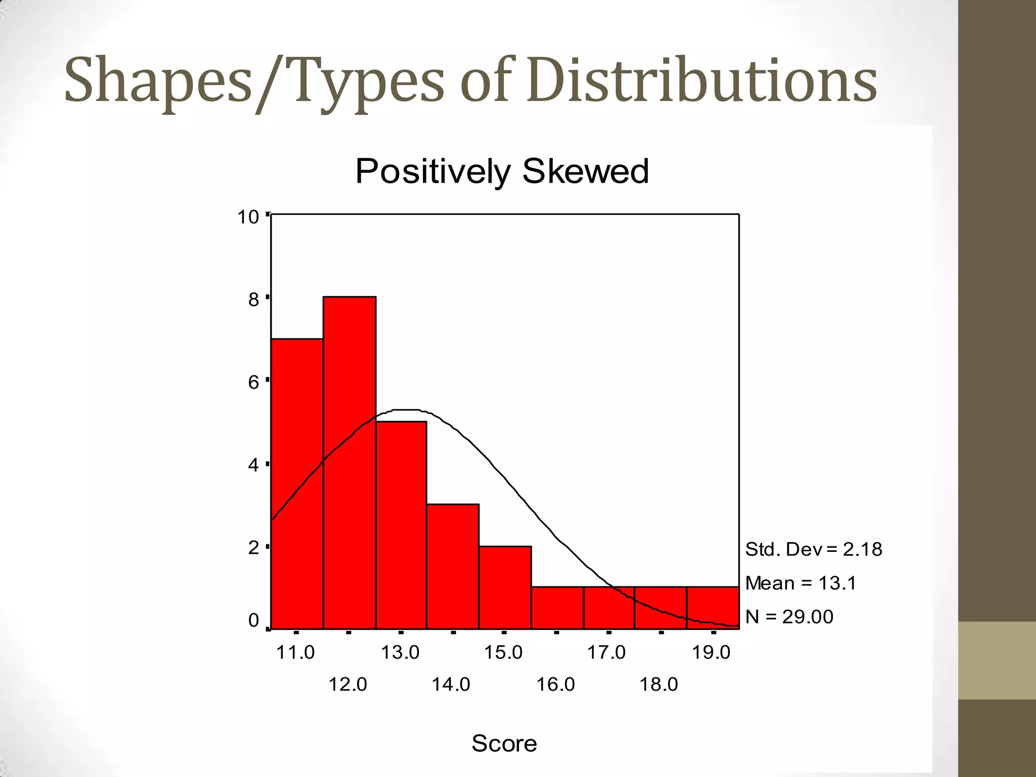
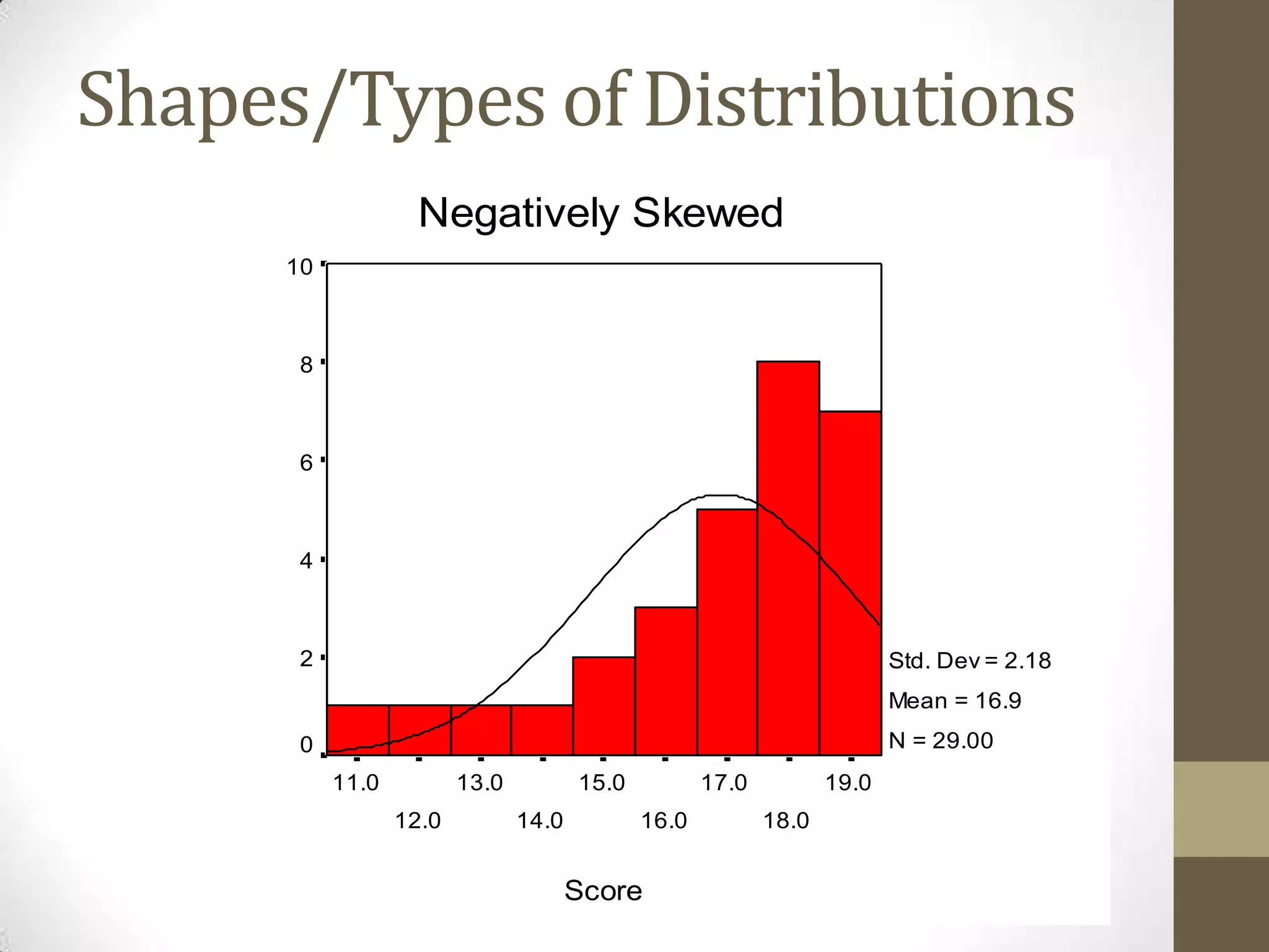
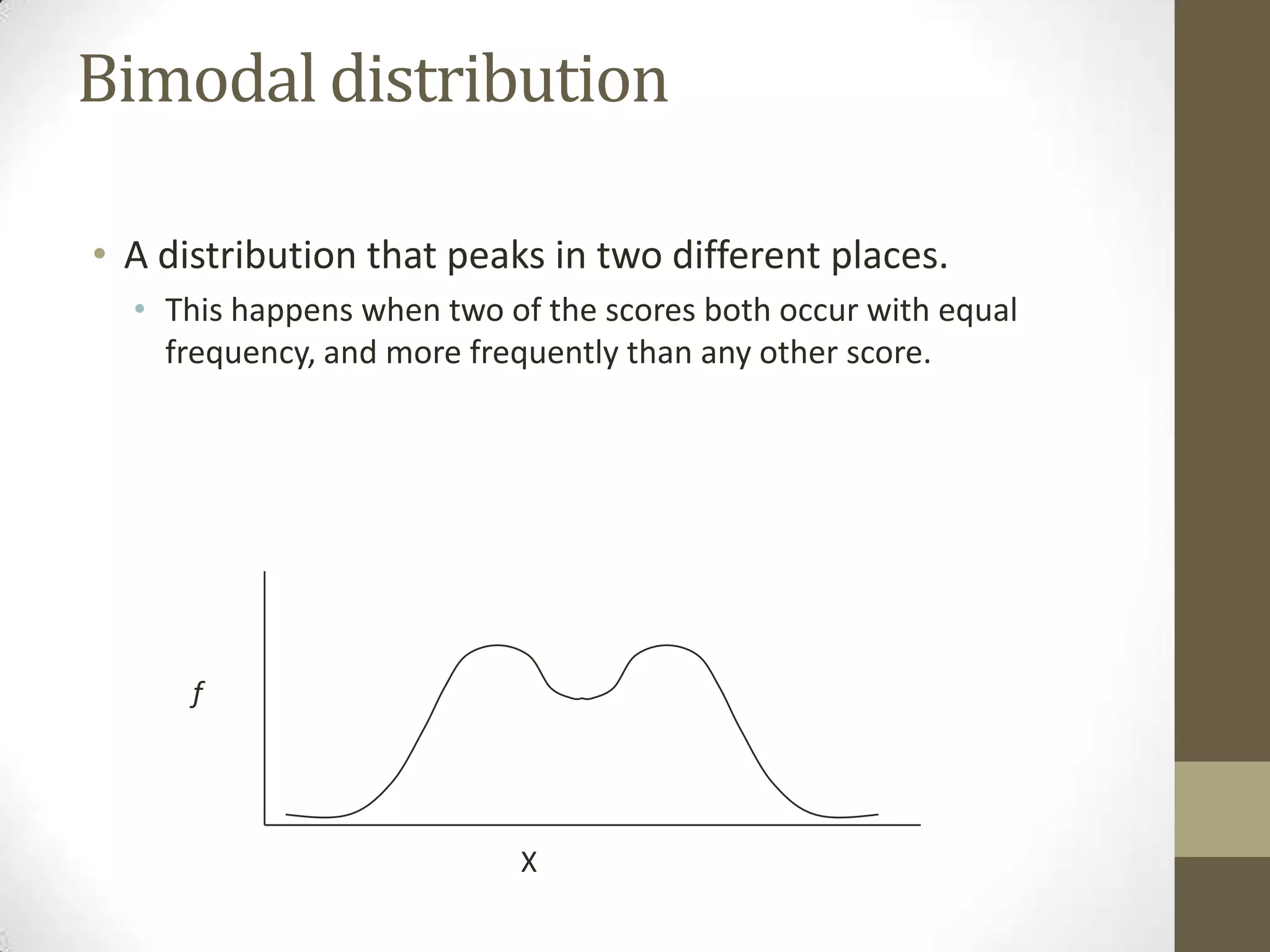
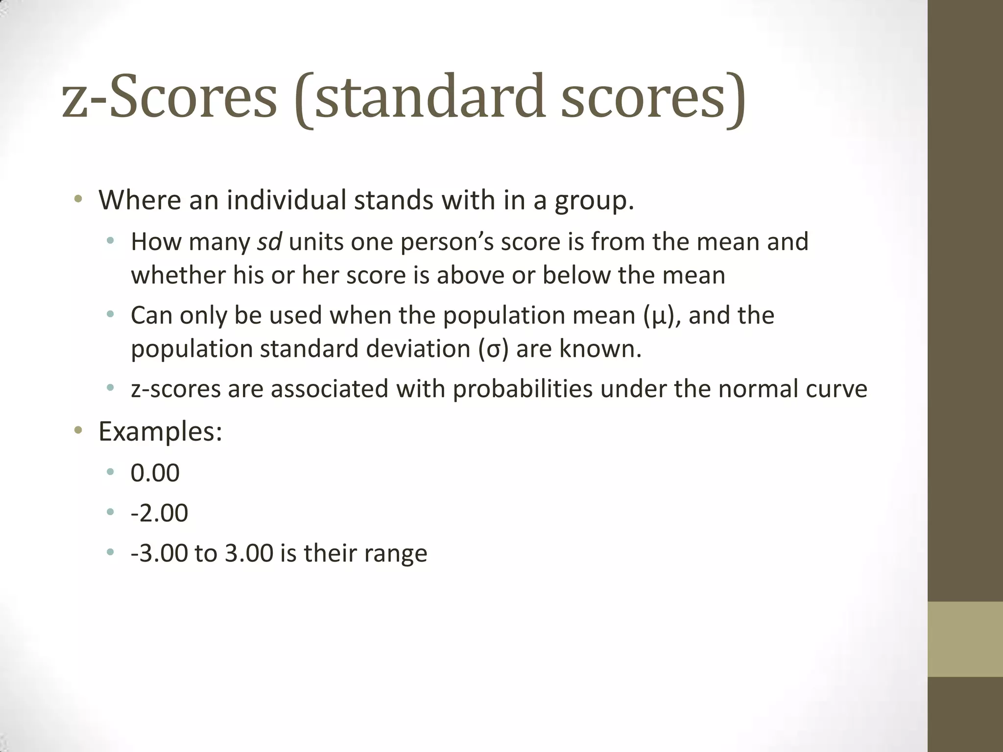
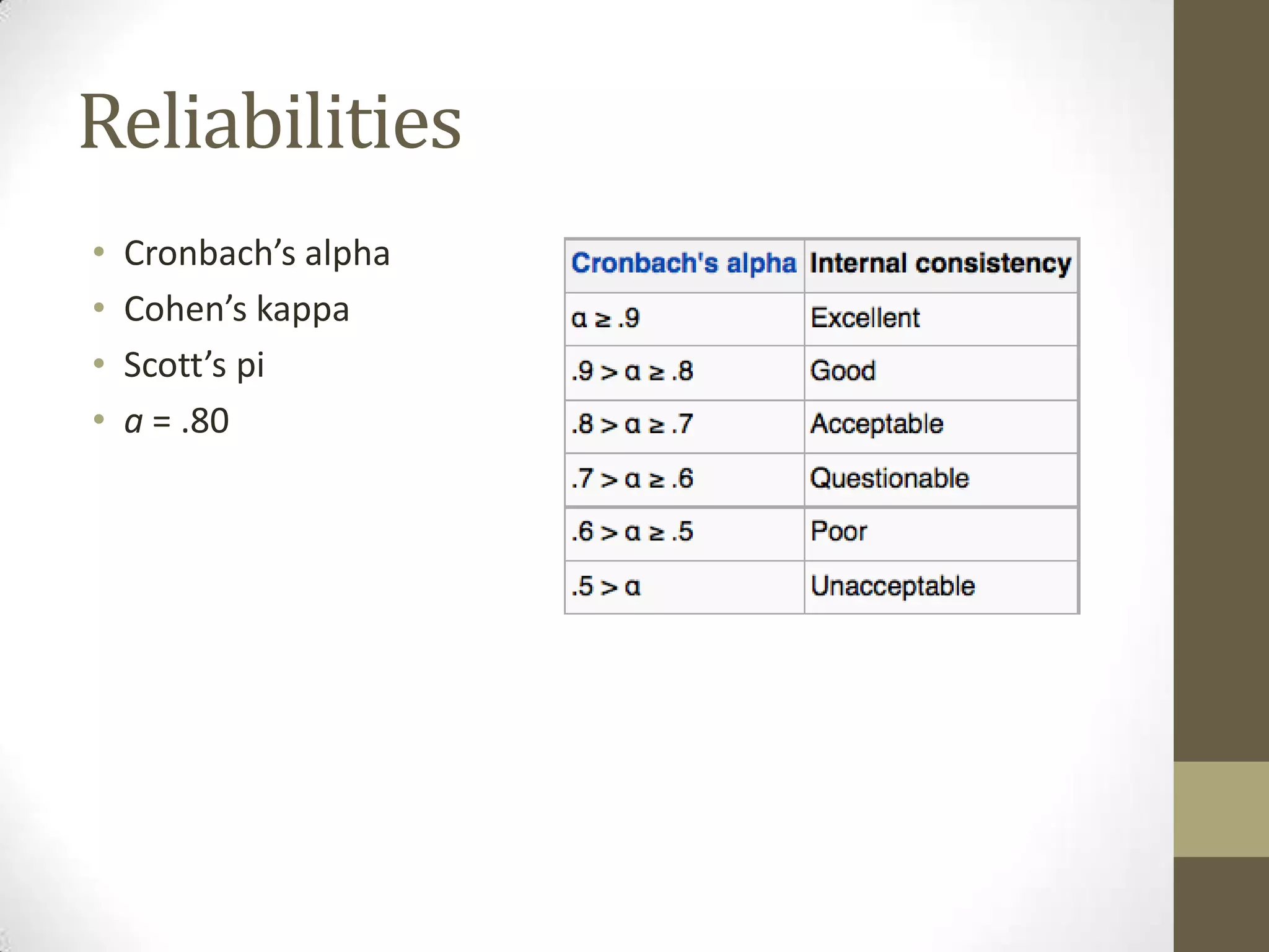
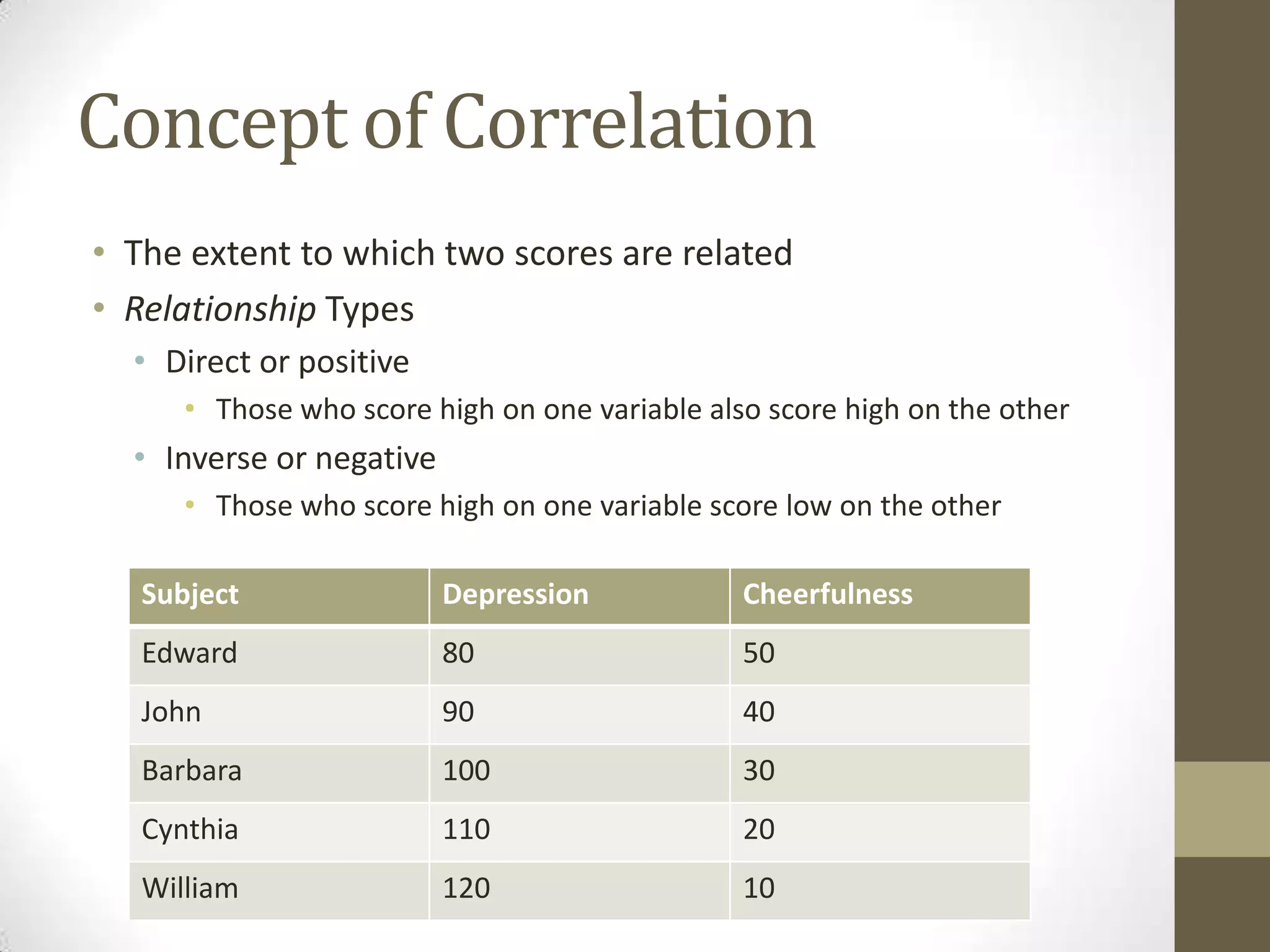
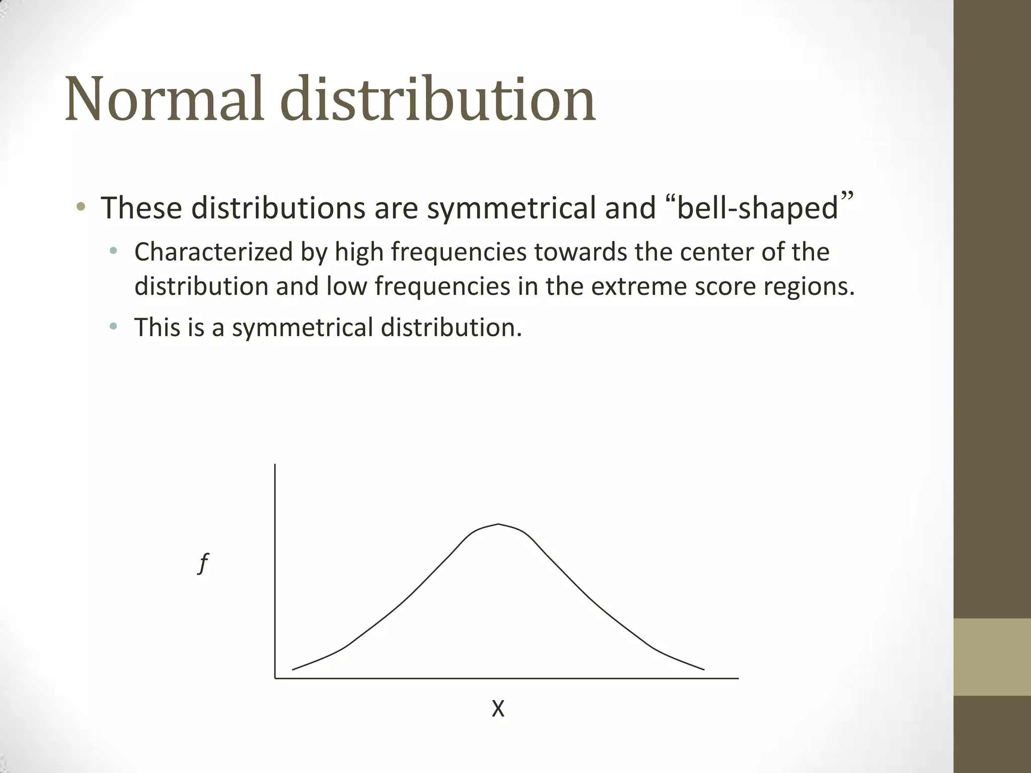
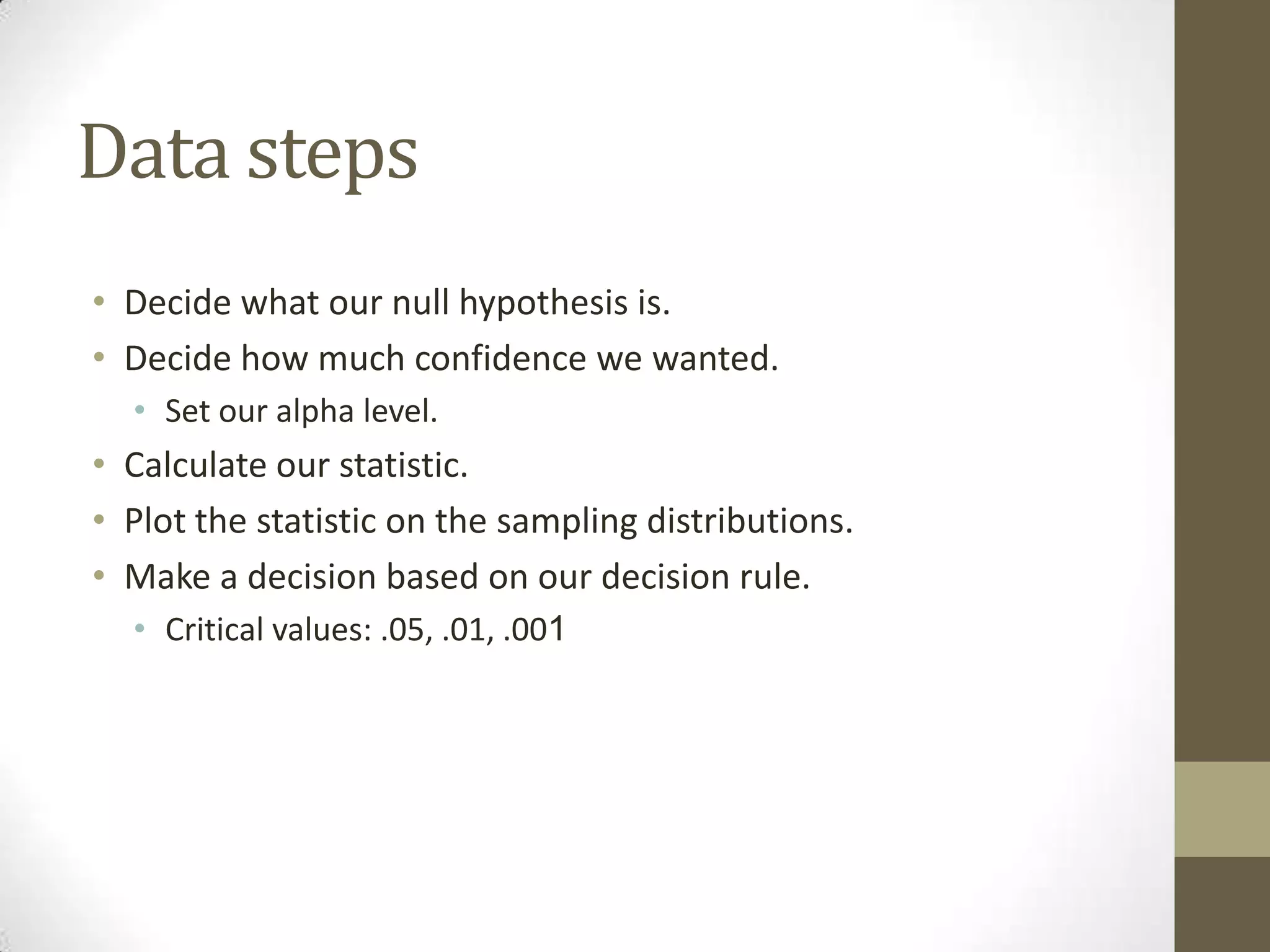
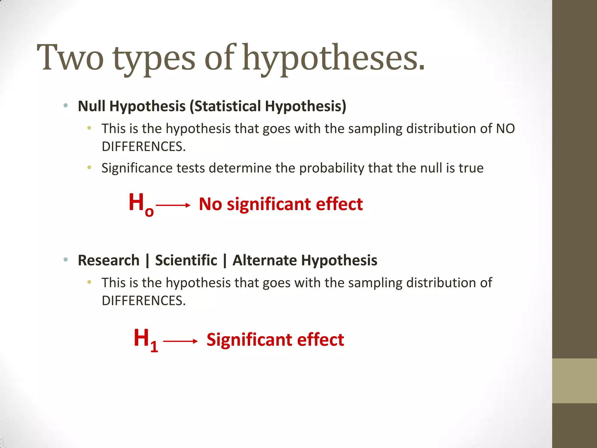
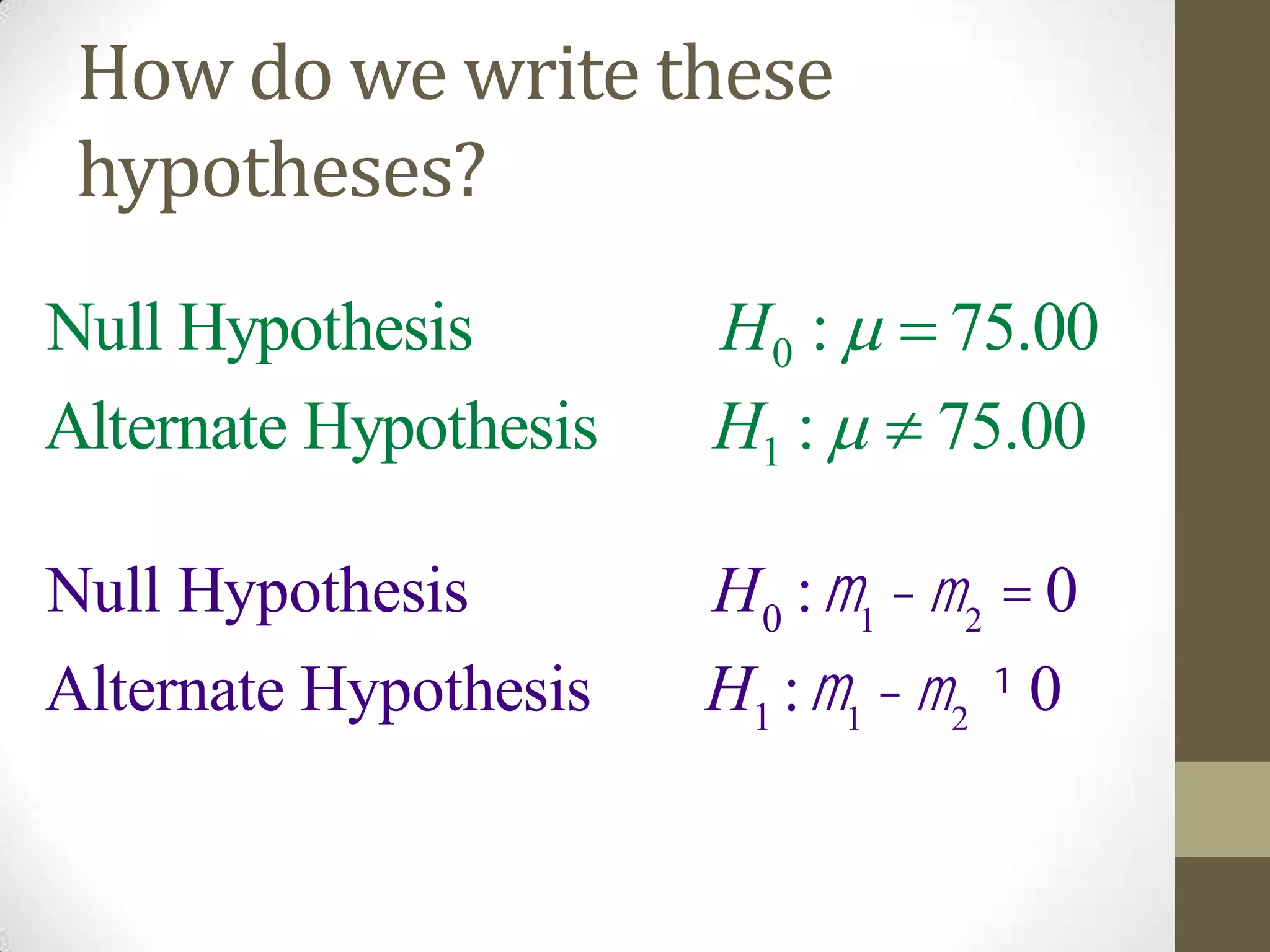
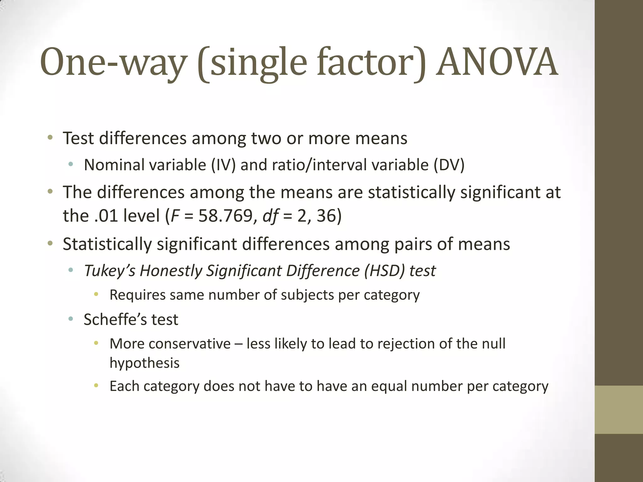
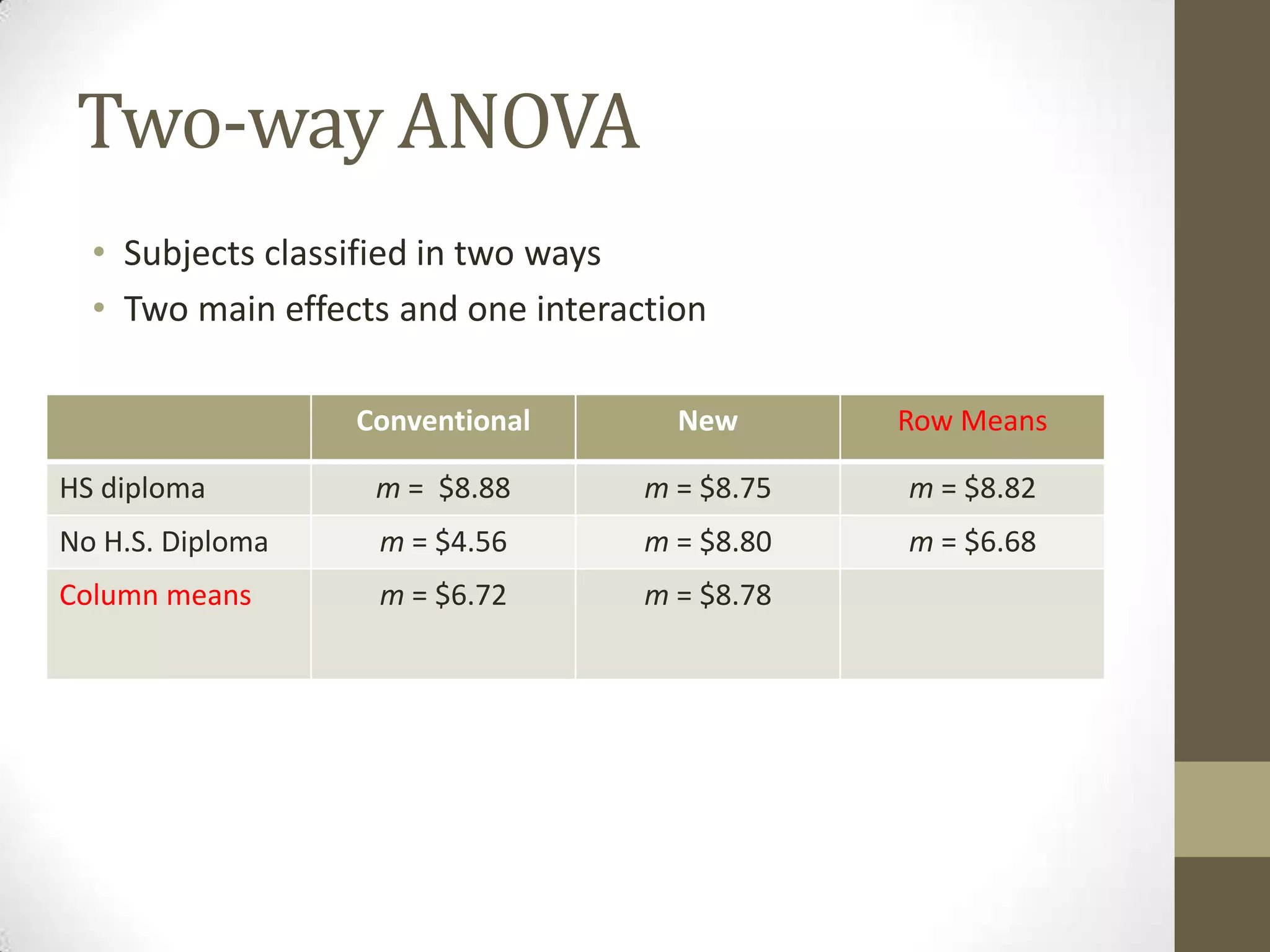
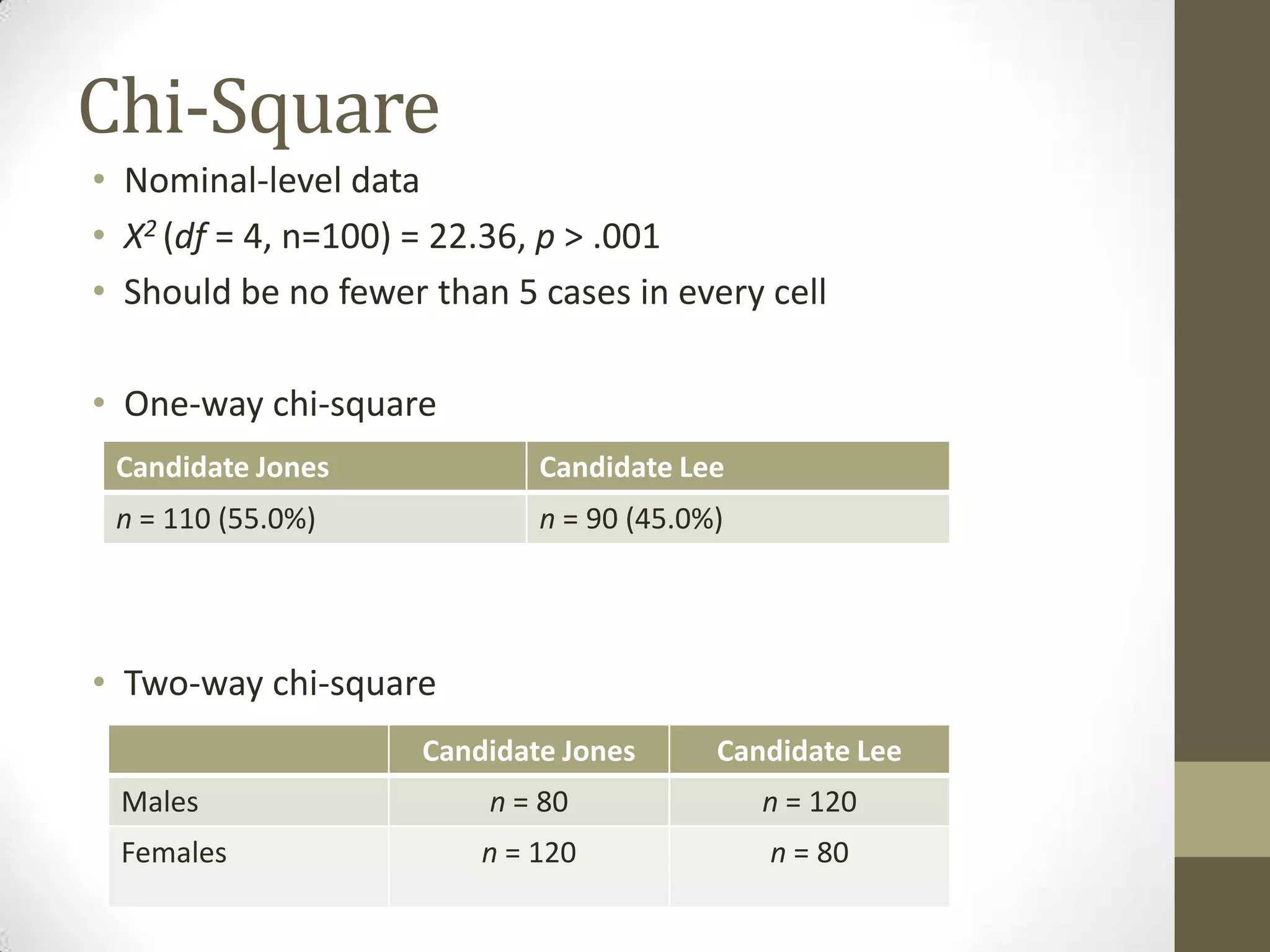
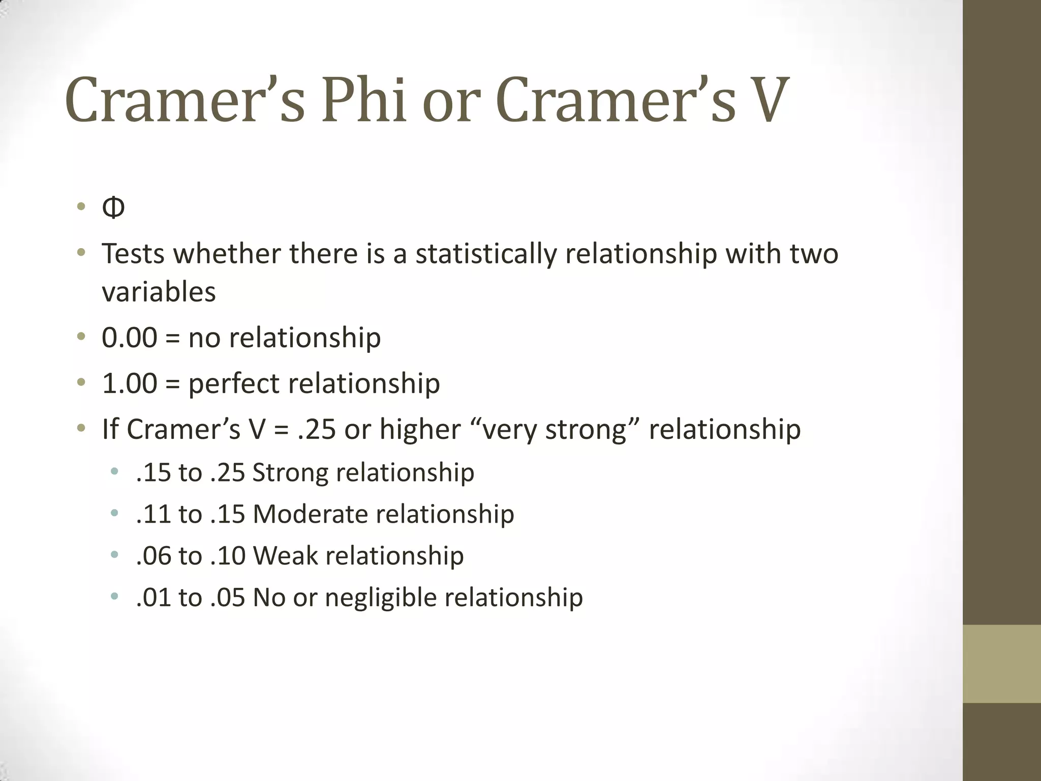
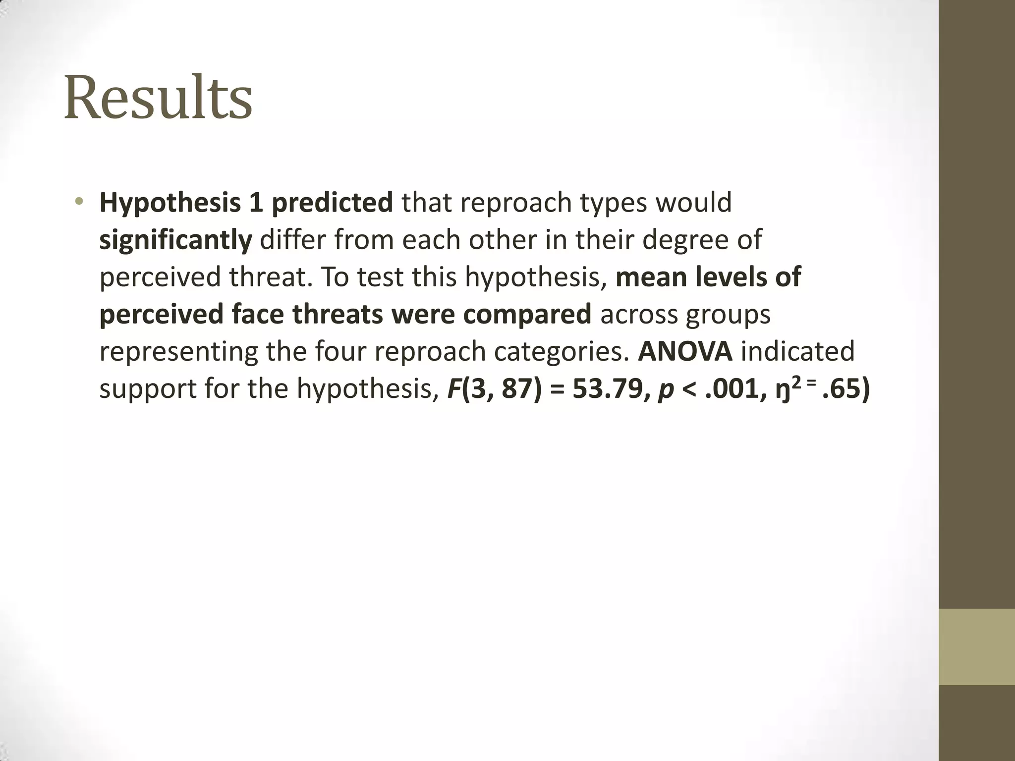
Descriptive &
Inferential Stats
By Serena Carpenter
Michigan State University
Parameter | Stats
• Parameter
• Describes a census and (stats) describe sample
• Nonparametric (categorical) stats
• Nominal and ordinal data
• Parametric (continuous) stats
• Interval and ratio
Descriptive | Inferential
• Descriptive
• Summarize data, sample
• In the beginning of the Results sections
• Inferential
• Generalize the sample data to a population
• Help researchers draw inferences about the effects of sampling
errors on the results
• Significance tests help researchers decide whether the
differences in descriptive statistics are reliable
Looking at my data
• Let’s say that you have a set of data:
• 5, 6, 4, 7, 3, 3, 7, 2, 1, 5, 3, 6
• How could you rearrange the data to get a better idea of what
the scores are in your data set?
• 1, 2, 3, 3, 3, 4, 5, 5, 6, 6, 7, 7
• How could you make it even more clear?
Frequency distribution
X f
7.00 2
6.00 2
5.00 2
4.00 1
3.00 3
2.00 1
1.00 1
f = 14(4%)
n = 14(4%)
Graphical Displays of Data
• Methods of graphing distributions:
• Histograms
• A frequency distribution where frequencies are represented
by bars.
• Stem-and-Leaf Displays
• An alternate way to represent a grouped frequency
distribution.
Grouped Frequency Histogram
Score (w = 3)
22.019.016.013.010.0
Frequency
25
20
15
10
5
0
Std. Dev = 3.01
Mean = 15.7
N = 47.00
Shapes/Types of Distributions
Score
19.0
18.0
17.0
16.0
15.0
14.0
13.0
12.0
11.0
Normal Distribution
Frequency
7
6
5
4
3
2
1
0
Std. Dev = 2.00
Mean = 15.0
N = 26.00
Shapes/Types of Distributions
Score
19.0
18.0
17.0
16.0
15.0
14.0
13.0
12.0
11.0
Positively Skewed
Frequency
10
8
6
4
2
0
Std. Dev = 2.18
Mean = 13.1
N = 29.00
Shapes/Types of Distributions
Score
19.0
18.0
17.0
16.0
15.0
14.0
13.0
12.0
11.0
Negatively Skewed
Frequency
10
8
6
4
2
0
Std. Dev = 2.18
Mean = 16.9
N = 29.00
Bimodal distribution
• A distribution that peaks in two different places.
• This happens when two of the scores both occur with equal
frequency, and more frequently than any other score.
X
f
Measures of Central Tendency
• Measures of central tendency help to give
information about the most likely score in a
distribution.
• We have three ways to describe central tendency:
• Mean
• Median
• Mode
Measures of Central Tendency
• Mean
• M or m
• Interval or ratio level
• Median
• Middle point of the distribution
• Insensitive to extreme scores. Use when the mean is
inappropriate.
• Mode
• Most frequently occurring
• The mode is appropriate for nominal scale data
Variability
• How much scores vary from each other
• Spread, dispersion
• Range
• 2, 3, 7, 7, 8, 8, 8, 12, 20
• Standard deviation
Standard deviation
• S, S.D., sd
• How much scores vary from the mean score
• About 2/3 of the case lie within one sd unit of the mean in a
normal distribution
S.D.
• 95% rule (precisely 1.96 sd units from the mean)
• 99.7% rule
• If M = 35.00 and S = 6.00, then:
• 68% cases lie between
29.00 and 41.00
• 95% cases lie between
23.00 and 47.00
• 99.7% cases lie between
17.00 and 53.00
z-Scores (standard scores)
• Where an individual stands with in a group.
• How many sd units one person’s score is from the mean and
whether his or her score is above or below the mean
• Can only be used when the population mean (μ), and the
population standard deviation (σ) are known.
• z-scores are associated with probabilities under the normal curve
• Examples:
• 0.00
• -2.00
• -3.00 to 3.00 is their range
Transformed Standard Scores
• z-Scores are transformed to another scale that does not have
0 as an average
• Many z-Transformations exist
Reliabilities
• Cronbach’s alpha
• Cohen’s kappa
• Scott’s pi
• a = .80
Concept of Correlation
• The extent to which two scores are related
• Relationship Types
• Direct or positive
• Those who score high on one variable also score high on the other
• Inverse or negative
• Those who score high on one variable score low on the other
Subject Depression Cheerfulness
Edward 80 50
John 90 40
Barbara 100 30
Cynthia 110 20
William 120 10
Causal relationship
• One variable causes a change in another variable
• Affects
• Controlled experiment in which one or more treatments are
administered
Linear regression - Scatterplot
• Graphic representation showing the relationship between two
variables
Pearson r
• Pearson product-moment correlation coefficient describes the
linear relationship between two scores (Likert/ratio)
• Ranges from -1.00 to 1.00
• -1.00 perfect negative relationship, 1.00 perfect positive
• No fewer than 25 participants
• Strong, moderate, weak
• +.40 to +.69 Strong positive relationship
+.30 to +.39 Moderate positive relationship
+.20 to +.29 weak positive relationship
+.01 to +.19 No or negligible relationship
-.01 to -.19 No or negligible relationship
-.20 to -.29 weak negative relationship
-.30 to -.39 Moderate negative relationship
-.40 to -.69 Strong negative relationship
-.70 or higher Very strong negative relationship
Coefficient of Determination
• To interpret Pearson r (r-squared)
• To interpret to what extent the variance of one variable
explains variance in another variable
• If Pearson r =-.77
• -.77 X -.77 X 100 = 59%
Spearman Rho rank correlation
• Ordinal or nominal
• -1.00 to 1.00
Alice Jordan Dexter Betty Ming
Math class 1 2 3 4 5
Philosophy 5 4 1 3 2
Normal distribution
• These distributions are symmetrical and “bell-shaped”
• Characterized by high frequencies towards the center of the
distribution and low frequencies in the extreme score regions.
• This is a symmetrical distribution.
f
X
Data steps
• Decide what our null hypothesis is.
• Decide how much confidence we wanted.
• Set our alpha level.
• Calculate our statistic.
• Plot the statistic on the sampling distributions.
• Make a decision based on our decision rule.
• Critical values: .05, .01, .001
Two types of hypotheses.
• Null Hypothesis (Statistical Hypothesis)
• This is the hypothesis that goes with the sampling distribution of NO
DIFFERENCES.
• Significance tests determine the probability that the null is true
• Research | Scientific | Alternate Hypothesis
• This is the hypothesis that goes with the sampling distribution of
DIFFERENCES.
H1 Significant effect
Ho No significant effect
How do we write these
hypotheses?
0
1
Null Hypothesis : 75.00
Alternate Hypothesis : 75.00
H
H




Null Hypothesis H0 :m1
-m2
= 0
Alternate Hypothesis H1 :m1
-m2
¹ 0
What do these hypotheses look like
conceptually?
0H1H 1H
This is our null distribution.
This is the one against which we will test
our sample.
We will specify the mean of this
population.
75.00 
Alpha and
significance level (probability)
• Significance level (p) p < .05
• Statistically significant
• The exact probability that the statistic we calculated on our
observed sample could actually occur in our null distribution
by chance alone.
• We can only calculate this if we have a computer.
• Alpha (α).
• The hypothetical remainder of the area under the curve other
than the CI.
• We decide on this level before we conduct the test.
• .05, .01, .001
Probability
• Two-tailed probability test
• Odds of drawing an individual at either tail of the normal distribution
• Flexibility
• Almost always select two-tailed test
• One-tailed probability test
• Easier to reject the null hypothesis – but in one and only direction
t test
• Compares the means of two samples for statistical significance
• One nominal variable with two categories and their scores on
one dependent interval/ratio variable
• t(4.62) = 2.17, p > .05
• Degrees of freedom
• df = n1 + n2 -2
• If the n=30 for one group and n=32 for another group, what is the
df for t test?
• (t=2.12, df=26, p <.05, two-tailed test)
One-way (single factor) ANOVA
• Test differences among two or more means
• Nominal variable (IV) and ratio/interval variable (DV)
• The differences among the means are statistically significant at
the .01 level (F = 58.769, df = 2, 36)
• Statistically significant differences among pairs of means
• Tukey’s Honestly Significant Difference (HSD) test
• Requires same number of subjects per category
• Scheffe’s test
• More conservative – less likely to lead to rejection of the null
hypothesis
• Each category does not have to have an equal number per category
Two-way ANOVA
• Subjects classified in two ways
• Two main effects and one interaction
Conventional New Row Means
HS diploma m = $8.88 m = $8.75 m = $8.82
No H.S. Diploma m = $4.56 m = $8.80 m = $6.68
Column means m = $6.72 m = $8.78
Chi-Square
• Nominal-level data
• X2 (df = 4, n=100) = 22.36, p > .001
• Should be no fewer than 5 cases in every cell
• One-way chi-square
• Two-way chi-square
Candidate Jones Candidate Lee
Males n = 80 n = 120
Females n = 120 n = 80
Candidate Jones Candidate Lee
n = 110 (55.0%) n = 90 (45.0%)
Cramer’s Phi or Cramer’s V
• Φ
• Tests whether there is a statistically relationship with two
variables
• 0.00 = no relationship
• 1.00 = perfect relationship
• If Cramer’s V = .25 or higher “very strong” relationship
• .15 to .25 Strong relationship
• .11 to .15 Moderate relationship
• .06 to .10 Weak relationship
• .01 to .05 No or negligible relationship
Results
• Hypothesis 1 predicted that reproach types would
significantly differ from each other in their degree of
perceived threat. To test this hypothesis, mean levels of
perceived face threats were compared across groups
representing the four reproach categories. ANOVA indicated
support for the hypothesis, F(3, 87) = 53.79, p < .001, ŋ2 = .65)
Agenda
• Intro to SPSS
• SPSS lecture and exercises. Held in 245
• Following week: No lecture
• April 25th
• Present for 5-10 minutes on your proposal.
• Feedback from the group
• May 1st
• Due by 2:45pm via email -

Stats - Intro to Quantitative

  • 1.
    Descriptive & Inferential Stats BySerena Carpenter Michigan State University
  • 2.
    Parameter | Stats •Parameter • Describes a census and (stats) describe sample • Nonparametric (categorical) stats • Nominal and ordinal data • Parametric (continuous) stats • Interval and ratio
  • 3.
    Descriptive | Inferential •Descriptive • Summarize data, sample • In the beginning of the Results sections • Inferential • Generalize the sample data to a population • Help researchers draw inferences about the effects of sampling errors on the results • Significance tests help researchers decide whether the differences in descriptive statistics are reliable
  • 4.
    Looking at mydata • Let’s say that you have a set of data: • 5, 6, 4, 7, 3, 3, 7, 2, 1, 5, 3, 6 • How could you rearrange the data to get a better idea of what the scores are in your data set? • 1, 2, 3, 3, 3, 4, 5, 5, 6, 6, 7, 7 • How could you make it even more clear?
  • 5.
    Frequency distribution X f 7.002 6.00 2 5.00 2 4.00 1 3.00 3 2.00 1 1.00 1 f = 14(4%) n = 14(4%)
  • 6.
    Graphical Displays ofData • Methods of graphing distributions: • Histograms • A frequency distribution where frequencies are represented by bars. • Stem-and-Leaf Displays • An alternate way to represent a grouped frequency distribution.
  • 7.
    Grouped Frequency Histogram Score(w = 3) 22.019.016.013.010.0 Frequency 25 20 15 10 5 0 Std. Dev = 3.01 Mean = 15.7 N = 47.00
  • 8.
    Shapes/Types of Distributions Score 19.0 18.0 17.0 16.0 15.0 14.0 13.0 12.0 11.0 NormalDistribution Frequency 7 6 5 4 3 2 1 0 Std. Dev = 2.00 Mean = 15.0 N = 26.00
  • 9.
    Shapes/Types of Distributions Score 19.0 18.0 17.0 16.0 15.0 14.0 13.0 12.0 11.0 PositivelySkewed Frequency 10 8 6 4 2 0 Std. Dev = 2.18 Mean = 13.1 N = 29.00
  • 10.
    Shapes/Types of Distributions Score 19.0 18.0 17.0 16.0 15.0 14.0 13.0 12.0 11.0 NegativelySkewed Frequency 10 8 6 4 2 0 Std. Dev = 2.18 Mean = 16.9 N = 29.00
  • 11.
    Bimodal distribution • Adistribution that peaks in two different places. • This happens when two of the scores both occur with equal frequency, and more frequently than any other score. X f
  • 12.
    Measures of CentralTendency • Measures of central tendency help to give information about the most likely score in a distribution. • We have three ways to describe central tendency: • Mean • Median • Mode
  • 13.
    Measures of CentralTendency • Mean • M or m • Interval or ratio level • Median • Middle point of the distribution • Insensitive to extreme scores. Use when the mean is inappropriate. • Mode • Most frequently occurring • The mode is appropriate for nominal scale data
  • 14.
    Variability • How muchscores vary from each other • Spread, dispersion • Range • 2, 3, 7, 7, 8, 8, 8, 12, 20 • Standard deviation
  • 15.
    Standard deviation • S,S.D., sd • How much scores vary from the mean score • About 2/3 of the case lie within one sd unit of the mean in a normal distribution
  • 16.
    S.D. • 95% rule(precisely 1.96 sd units from the mean) • 99.7% rule • If M = 35.00 and S = 6.00, then: • 68% cases lie between 29.00 and 41.00 • 95% cases lie between 23.00 and 47.00 • 99.7% cases lie between 17.00 and 53.00
  • 17.
    z-Scores (standard scores) •Where an individual stands with in a group. • How many sd units one person’s score is from the mean and whether his or her score is above or below the mean • Can only be used when the population mean (μ), and the population standard deviation (σ) are known. • z-scores are associated with probabilities under the normal curve • Examples: • 0.00 • -2.00 • -3.00 to 3.00 is their range
  • 18.
    Transformed Standard Scores •z-Scores are transformed to another scale that does not have 0 as an average • Many z-Transformations exist
  • 19.
    Reliabilities • Cronbach’s alpha •Cohen’s kappa • Scott’s pi • a = .80
  • 20.
    Concept of Correlation •The extent to which two scores are related • Relationship Types • Direct or positive • Those who score high on one variable also score high on the other • Inverse or negative • Those who score high on one variable score low on the other Subject Depression Cheerfulness Edward 80 50 John 90 40 Barbara 100 30 Cynthia 110 20 William 120 10
  • 21.
    Causal relationship • Onevariable causes a change in another variable • Affects • Controlled experiment in which one or more treatments are administered
  • 22.
    Linear regression -Scatterplot • Graphic representation showing the relationship between two variables
  • 23.
    Pearson r • Pearsonproduct-moment correlation coefficient describes the linear relationship between two scores (Likert/ratio) • Ranges from -1.00 to 1.00 • -1.00 perfect negative relationship, 1.00 perfect positive • No fewer than 25 participants • Strong, moderate, weak • +.40 to +.69 Strong positive relationship +.30 to +.39 Moderate positive relationship +.20 to +.29 weak positive relationship +.01 to +.19 No or negligible relationship -.01 to -.19 No or negligible relationship -.20 to -.29 weak negative relationship -.30 to -.39 Moderate negative relationship -.40 to -.69 Strong negative relationship -.70 or higher Very strong negative relationship
  • 24.
    Coefficient of Determination •To interpret Pearson r (r-squared) • To interpret to what extent the variance of one variable explains variance in another variable • If Pearson r =-.77 • -.77 X -.77 X 100 = 59%
  • 25.
    Spearman Rho rankcorrelation • Ordinal or nominal • -1.00 to 1.00 Alice Jordan Dexter Betty Ming Math class 1 2 3 4 5 Philosophy 5 4 1 3 2
  • 26.
    Normal distribution • Thesedistributions are symmetrical and “bell-shaped” • Characterized by high frequencies towards the center of the distribution and low frequencies in the extreme score regions. • This is a symmetrical distribution. f X
  • 27.
    Data steps • Decidewhat our null hypothesis is. • Decide how much confidence we wanted. • Set our alpha level. • Calculate our statistic. • Plot the statistic on the sampling distributions. • Make a decision based on our decision rule. • Critical values: .05, .01, .001
  • 28.
    Two types ofhypotheses. • Null Hypothesis (Statistical Hypothesis) • This is the hypothesis that goes with the sampling distribution of NO DIFFERENCES. • Significance tests determine the probability that the null is true • Research | Scientific | Alternate Hypothesis • This is the hypothesis that goes with the sampling distribution of DIFFERENCES. H1 Significant effect Ho No significant effect
  • 29.
    How do wewrite these hypotheses? 0 1 Null Hypothesis : 75.00 Alternate Hypothesis : 75.00 H H     Null Hypothesis H0 :m1 -m2 = 0 Alternate Hypothesis H1 :m1 -m2 ¹ 0
  • 30.
    What do thesehypotheses look like conceptually? 0H1H 1H This is our null distribution. This is the one against which we will test our sample. We will specify the mean of this population. 75.00 
  • 31.
    Alpha and significance level(probability) • Significance level (p) p < .05 • Statistically significant • The exact probability that the statistic we calculated on our observed sample could actually occur in our null distribution by chance alone. • We can only calculate this if we have a computer. • Alpha (α). • The hypothetical remainder of the area under the curve other than the CI. • We decide on this level before we conduct the test. • .05, .01, .001
  • 32.
    Probability • Two-tailed probabilitytest • Odds of drawing an individual at either tail of the normal distribution • Flexibility • Almost always select two-tailed test • One-tailed probability test • Easier to reject the null hypothesis – but in one and only direction
  • 33.
    t test • Comparesthe means of two samples for statistical significance • One nominal variable with two categories and their scores on one dependent interval/ratio variable • t(4.62) = 2.17, p > .05 • Degrees of freedom • df = n1 + n2 -2 • If the n=30 for one group and n=32 for another group, what is the df for t test? • (t=2.12, df=26, p <.05, two-tailed test)
  • 34.
    One-way (single factor)ANOVA • Test differences among two or more means • Nominal variable (IV) and ratio/interval variable (DV) • The differences among the means are statistically significant at the .01 level (F = 58.769, df = 2, 36) • Statistically significant differences among pairs of means • Tukey’s Honestly Significant Difference (HSD) test • Requires same number of subjects per category • Scheffe’s test • More conservative – less likely to lead to rejection of the null hypothesis • Each category does not have to have an equal number per category
  • 35.
    Two-way ANOVA • Subjectsclassified in two ways • Two main effects and one interaction Conventional New Row Means HS diploma m = $8.88 m = $8.75 m = $8.82 No H.S. Diploma m = $4.56 m = $8.80 m = $6.68 Column means m = $6.72 m = $8.78
  • 36.
    Chi-Square • Nominal-level data •X2 (df = 4, n=100) = 22.36, p > .001 • Should be no fewer than 5 cases in every cell • One-way chi-square • Two-way chi-square Candidate Jones Candidate Lee Males n = 80 n = 120 Females n = 120 n = 80 Candidate Jones Candidate Lee n = 110 (55.0%) n = 90 (45.0%)
  • 37.
    Cramer’s Phi orCramer’s V • Φ • Tests whether there is a statistically relationship with two variables • 0.00 = no relationship • 1.00 = perfect relationship • If Cramer’s V = .25 or higher “very strong” relationship • .15 to .25 Strong relationship • .11 to .15 Moderate relationship • .06 to .10 Weak relationship • .01 to .05 No or negligible relationship
  • 38.
    Results • Hypothesis 1predicted that reproach types would significantly differ from each other in their degree of perceived threat. To test this hypothesis, mean levels of perceived face threats were compared across groups representing the four reproach categories. ANOVA indicated support for the hypothesis, F(3, 87) = 53.79, p < .001, ŋ2 = .65)
  • 39.
    Agenda • Intro toSPSS • SPSS lecture and exercises. Held in 245 • Following week: No lecture • April 25th • Present for 5-10 minutes on your proposal. • Feedback from the group • May 1st • Due by 2:45pm via email -

Editor's Notes

  • #3 Average for a census should be referred to as a parameter, but average for a sample is a statistic. You must understand stats in order to understand how to write your Hypotheses and RQs/.
  • #4 Instead of presenting a list of 500 scores, you might present the average
  • #14 The most popular is the average… however there are several types of averages in statsBecause it is dependent upon the magnitude of scores. If all scores are the same then there is no Mode. If two adjacent scores both have the same, and the highest frequency, then the Mode is the average between the two scores
  • #15 How much individuals vary is important for statistical and practical reasons. Average is an abstraction… we are more interested in variability (who and who does not)… what causes variations. Suppose you had to chose between two classes with the same average, however in one class that test scores varied greatly from highest to lowest? Which class would be easiest to teach for? A simple statistic to describe variability is a range. A weakness though is that it only reports two scores. 2-20. However, you will notice that there is an outlier. Which number is the outlier? The outlier greatly increases the range.As a simple example, consider the average daily high temperatures for two cities, one inland and one near the ocean. It is helpful to understand that the range of daily high temperatures for cities near the ocean is smaller than for cities inland. These two cities may each have the same average high temperature. However, the standard deviation of the daily high temperature for the coastal city will be less than that of the inland city .
  • #16 The amount by which participants vary or differ from each other.The larger the deviation from the mean, the larger the sd… the greater variabilityYou are calculating the number of points that one must go out form the mean to capture 68% of the cases. Very diverse samples you have have to go further out to capture 68% of the cases. A low standard deviation means that most of the numbers are very close to the average
  • #17 It says approximately 95% of the case lie within 2 sd of mean in a normal distribution3 sd units from means. In a NORMAL distribution has only 6 sd units – 3 above and 3 below.. Keep in mind the sd is used to compute the variability of the scoresLet&apos;s say your teacher gives a test to one hundred kids and the test average is 80 points and the S.D. is 10. If the distribution is &quot;normal,&quot; about 34 kids will score between 70 and 80, and about 34 kids will score between 80 and 90. We can also predict that about 14 kids will score between 90 and 100, and 14 will score below 70.
  • #19 If a person has been told that they performed 0.00 (THE AVERAGE) on test, they would like be confused or if some received a -1.0. To get around this problem, z-scores are transformed to another scale that does not have 0 as an average. 40 is 1 sd below the mean
  • #20 Ratio level variables – internal consistency… subitems on a scale do they relateinternal consistency is typically a measure based on the correlations between different items on the same test (or the same subscale on a larger test). It measures whether several items that propose to measure the same general construct produce similar scores… An alternative way of thinking about internal consistency is that it is the extent to which all of the items of a test measure the same latent variable. internal consistency ranges from 0 to 1Scotts pi done to check interrater reliability of of nominal and ordinal level variables for content analysis
  • #21 The scores in the box indicate what type of relationship? Inverse
  • #22 Correlations can hint at causality, which can later be explored in experiments.
  • #23 One dot for each subject. If the pattern is very clear, there relationship is very strong. It would be an inverse relationship if it went in the other direction Linear relationship between variables… hat is, as height increases so does basketball performance.Extreme scatter means no relationship exists… or a very weak relationship
  • #24 To statistically determine whether a relationship exists… use a Pearson correlation coefficient. The closer the dots, the stronger the relationship. How do you know if a relationship exists? And what is the strength of the relationship?
  • #25 59% of the variance of one variable is accounted by the variance of another. And that means 41% of the variance is not accounted for…. Remember our variables must vary… and there is much room for improvement
  • #26 NoPearsons is for ratio or interval level data….. Five college students&apos; have the following rankings in math and science courses. Is there an association between the rankings in math and science courses. Ranking of news values how two groups rank them
  • #33 We are open to the results going in either directionWe are certain that the results will only go in one direction and are not interested in either directionOne-tailed are frowned upon. Convinced your audience would not be interested if differences went other direction. Vitamin E relates to decrease in wrinkles… but suppose that the one who took it increased in wrinkles, wouldn’t we want to know that?
  • #34 Difference in whether male and female voters in their attitudes toward welfareThe DV must be interval/ratio and IV must be a nominal variable60degrees of freedom is the number of values in the final calculation of a statistic that are free to vary
  • #35 Three groups treated for migraine medicine 250 milligrams, 100 miligrams, placebo… there are three differences among meansBoth are acceptable, however a consumer of researcher may be more comfortable with the rejection of the null with more conservative testF = t squared, degrees of freedomIt is used in conjunction with an ANOVA to find means that are significantly different from each other
  • #36 Whereas one-way analysis of variance (ANOVA) tests measure significant effects ofone factor only, two-way analysis of variance (ANOVA) tests (also called two-factoranalysis of variance) measure the effects of two factors simultaneously. Drug groups and whether he or she is male or female. New job training program. Whether they had a high school diploma. Mean hourly wages,. Overall the new program is superior to the conventioal one. The difference is $8.78 – $6.72=$2.06 suggests there is a main effect.
  • #37 Chi-square is a difference test, whether a difference occurs between two groups…. You can legitimately say that a difference exists. A chi-square to assess whether females and males differ in their political affiliation. Analysis does not permit the computation of means and standard deviations= calculated value,
  • #38 Effect size…. Cramer&apos;s V is a way of calculating correlation in tables which have more than 2x2 rows and columns. It is used as post-test to determine strengths of association after chi-square has determined significance.  Strengthof the association between two variables the intercorrelation of two discrete variables[2] and may be used with variables having two or more levels.Probability level and effect size
  • #39 Paragraph of descriptivesOne paragraph to overviewing the stats. Remind the audience of your hypothesesStatement describing the test employedThe calculated statWhether the outcome was significantEta-squared ---- measure the strength of the relationship of interest (effect size) p values says that there is relationship whereas additional statistical analysis tells use the magnitude of the relationship.. R-squared, eta-squared, and cramers v