The document discusses various statistical concepts related to hypothesis testing including:
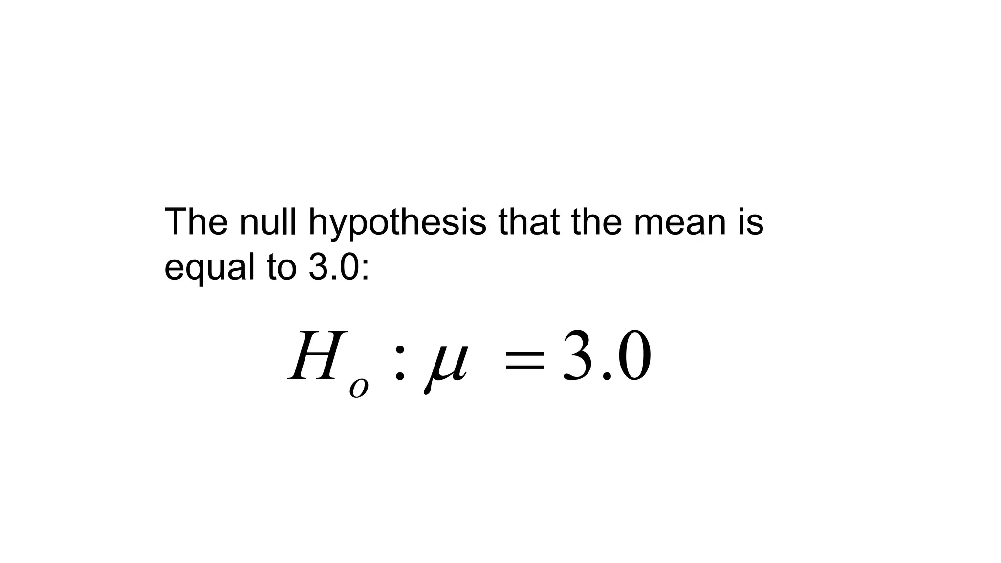
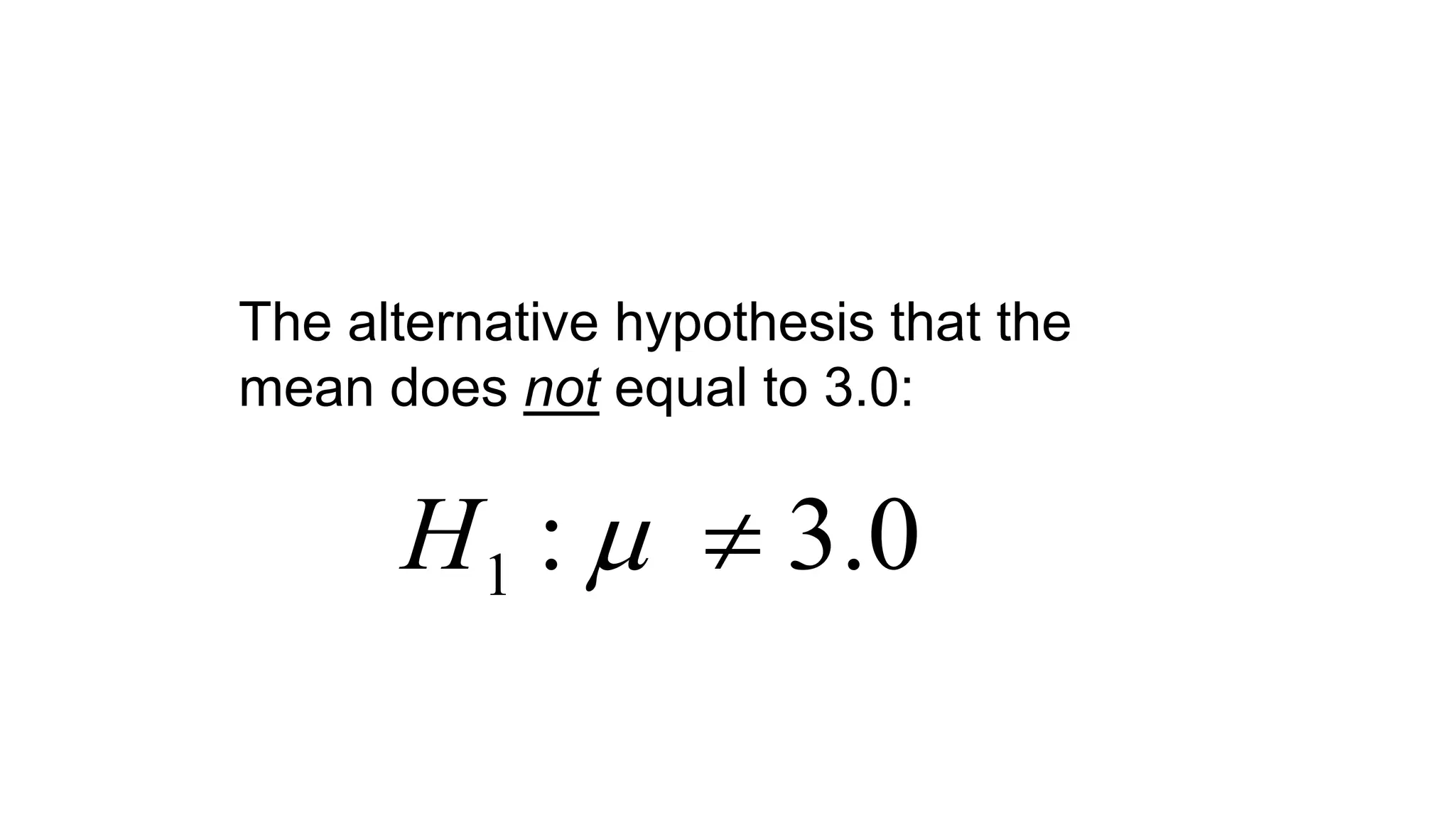
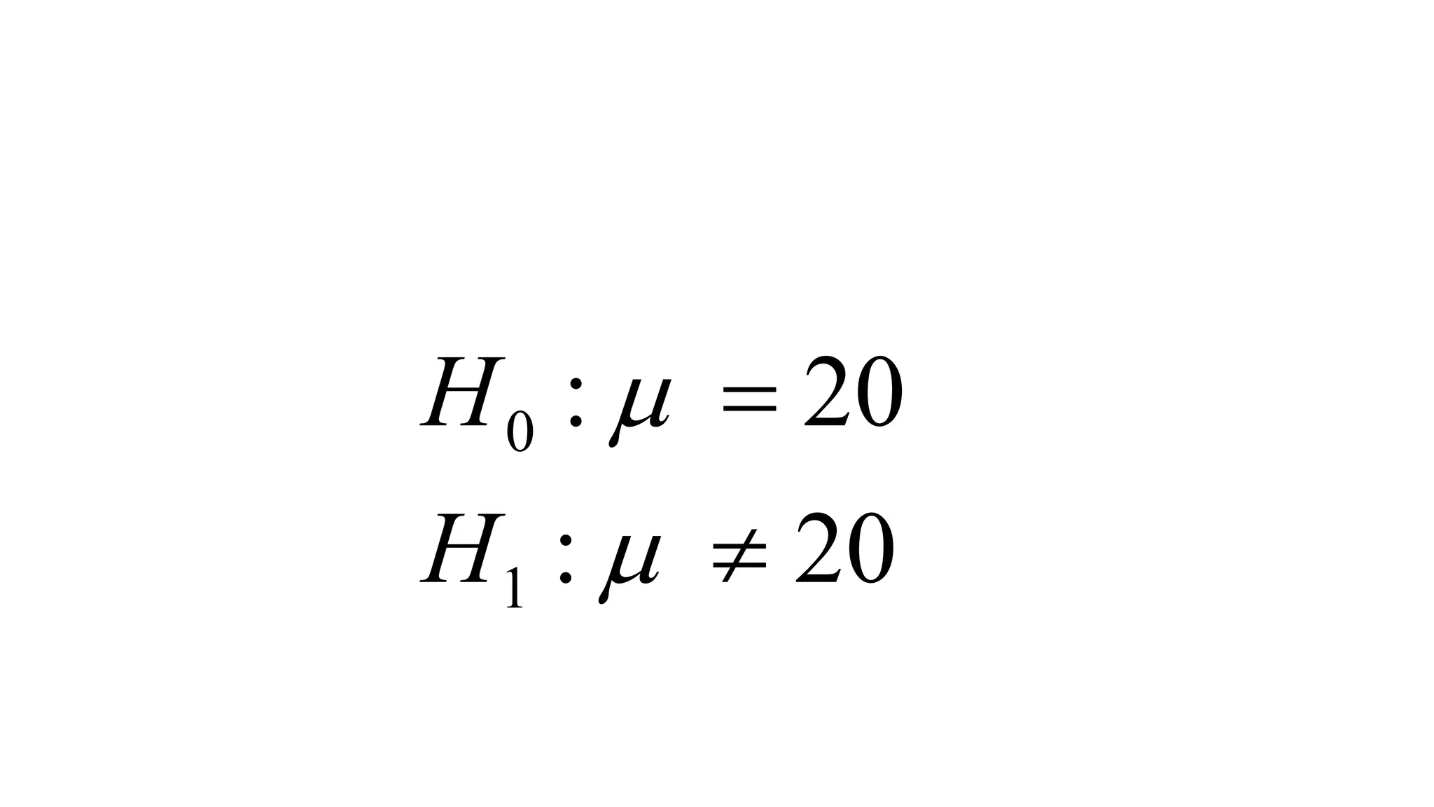
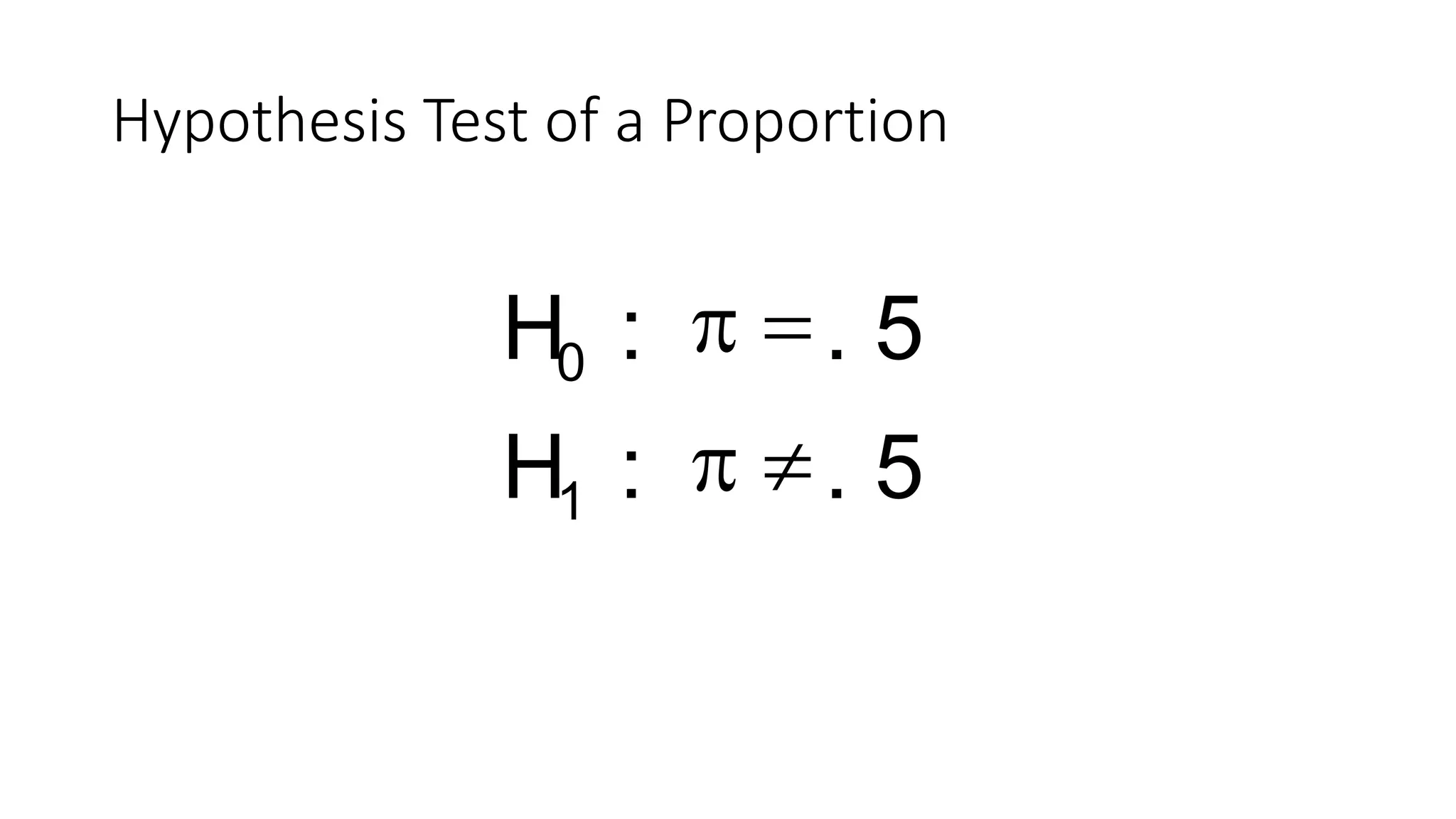
- Hypothesis, null hypothesis, and alternative hypothesis
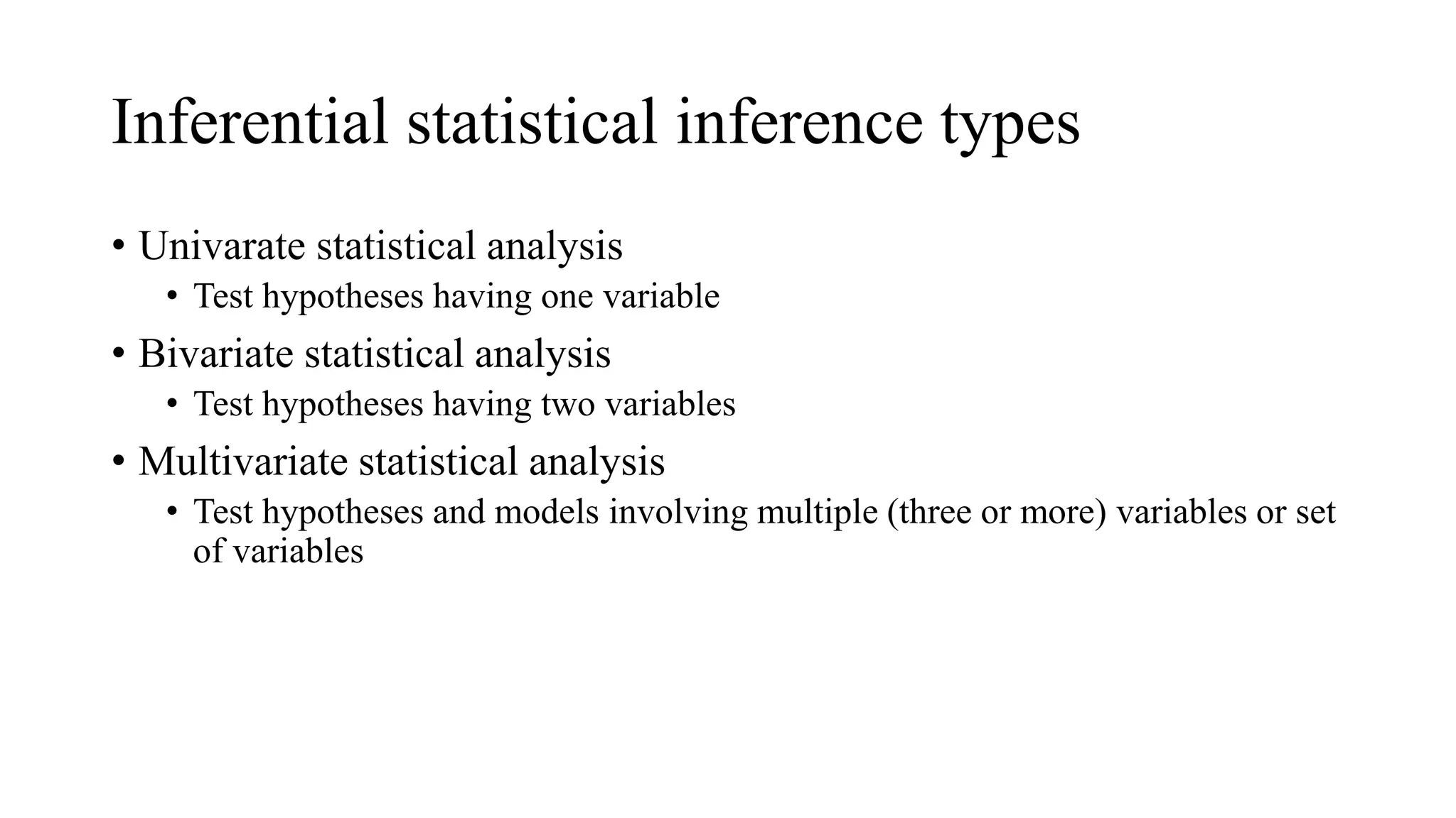
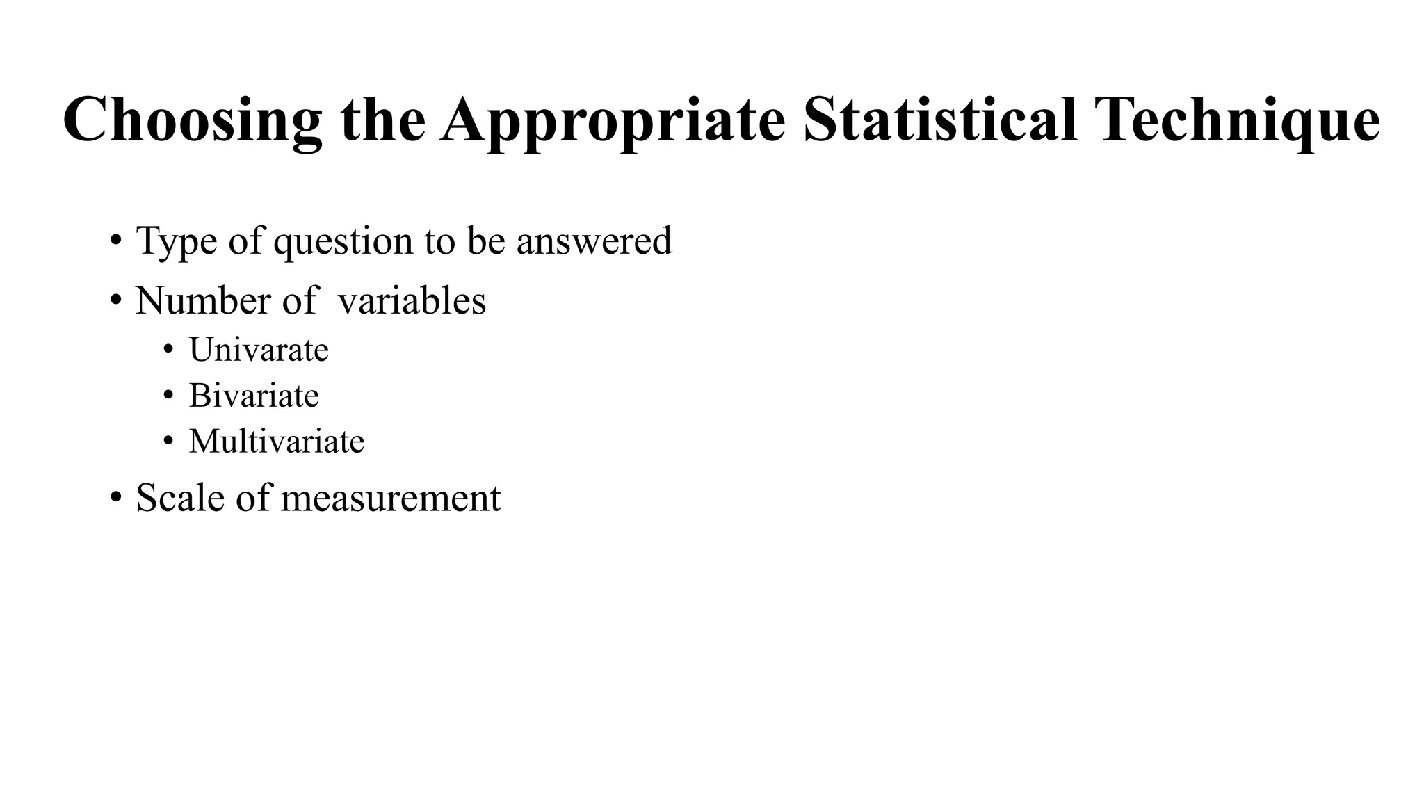
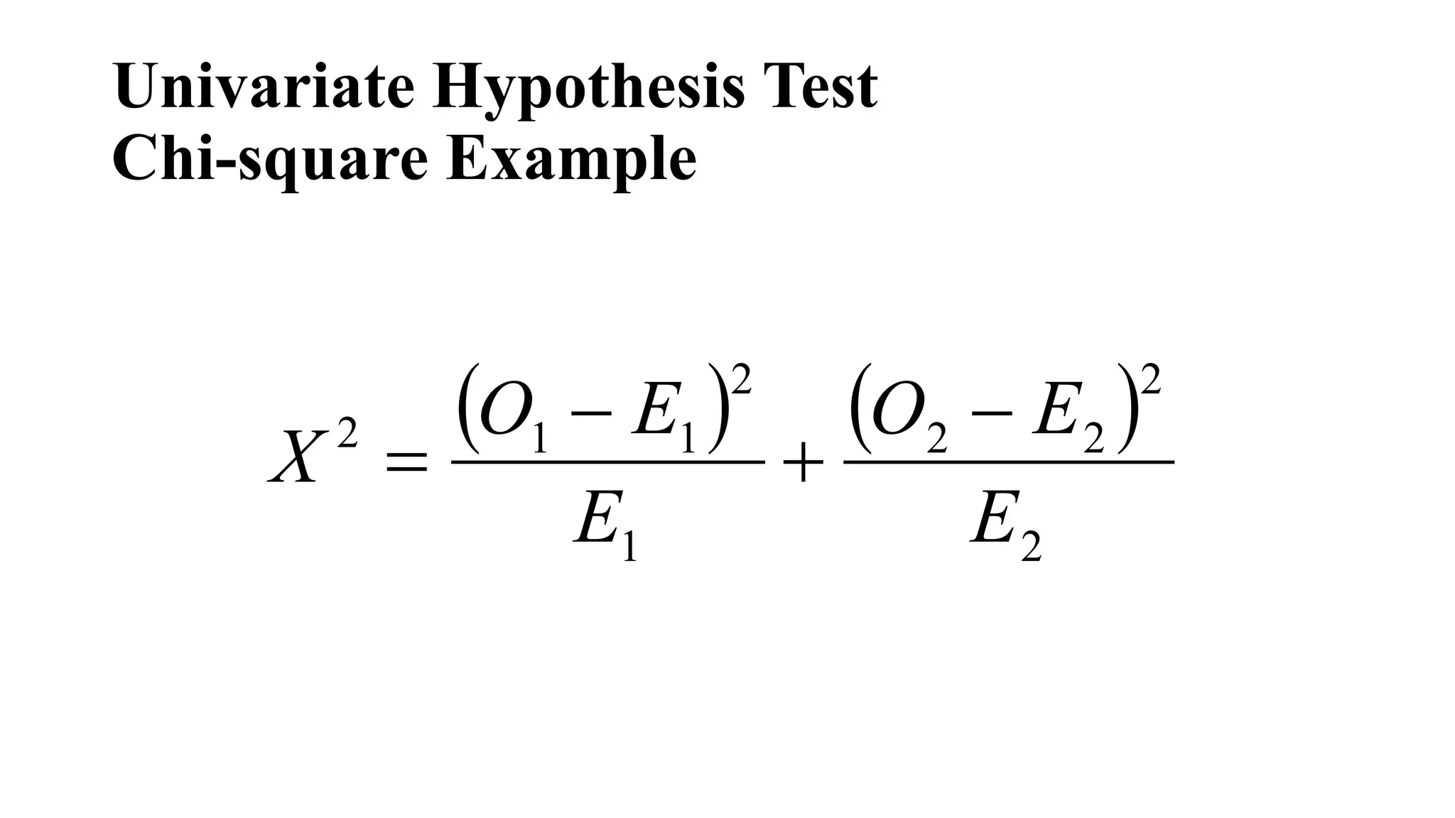
- Types of statistical analyses for testing hypotheses (univariate, bivariate, multivariate)
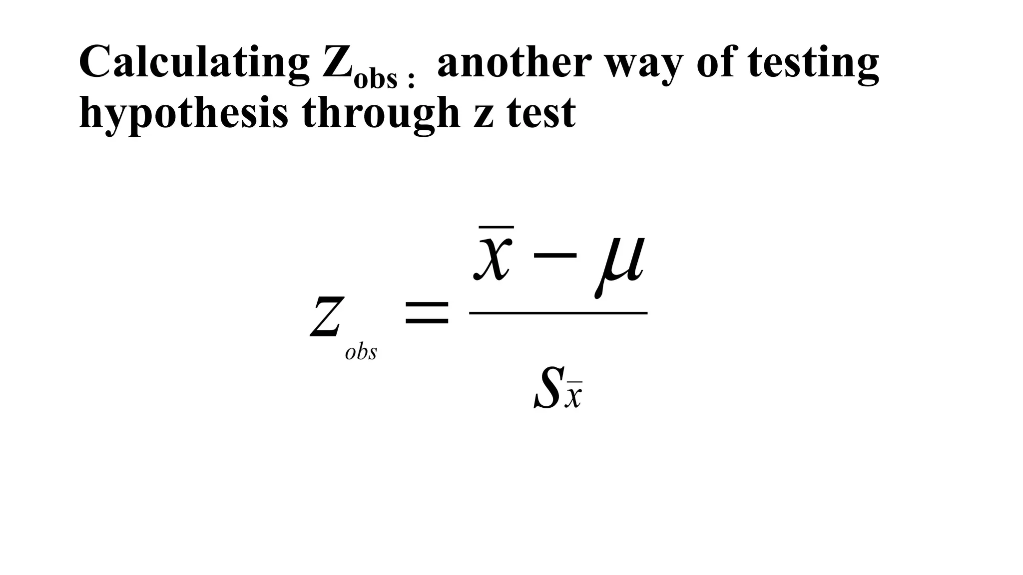
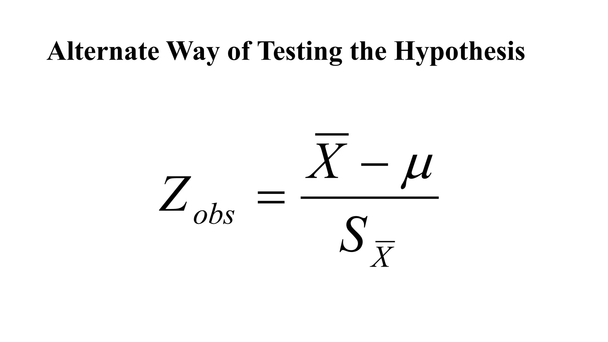
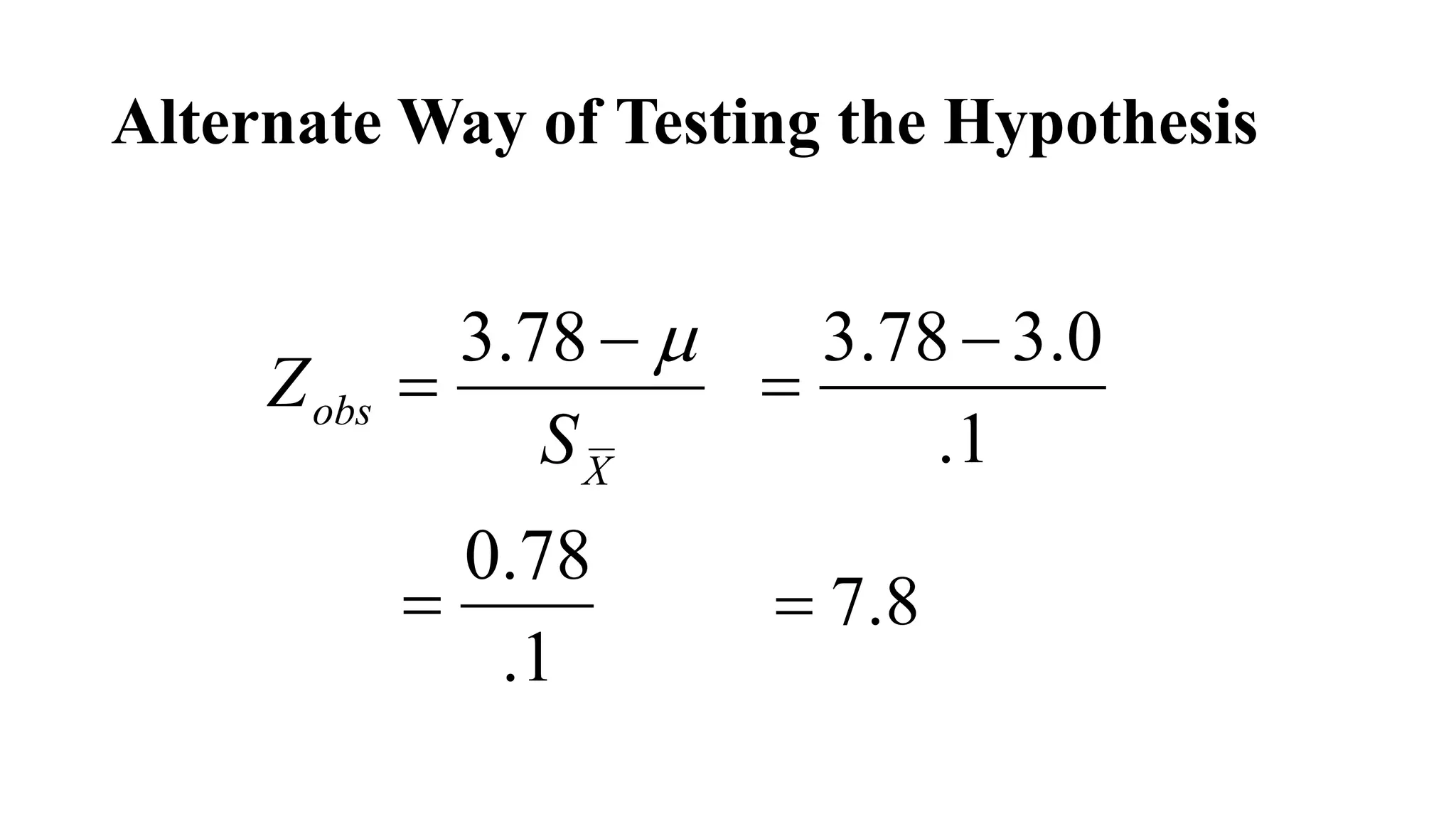
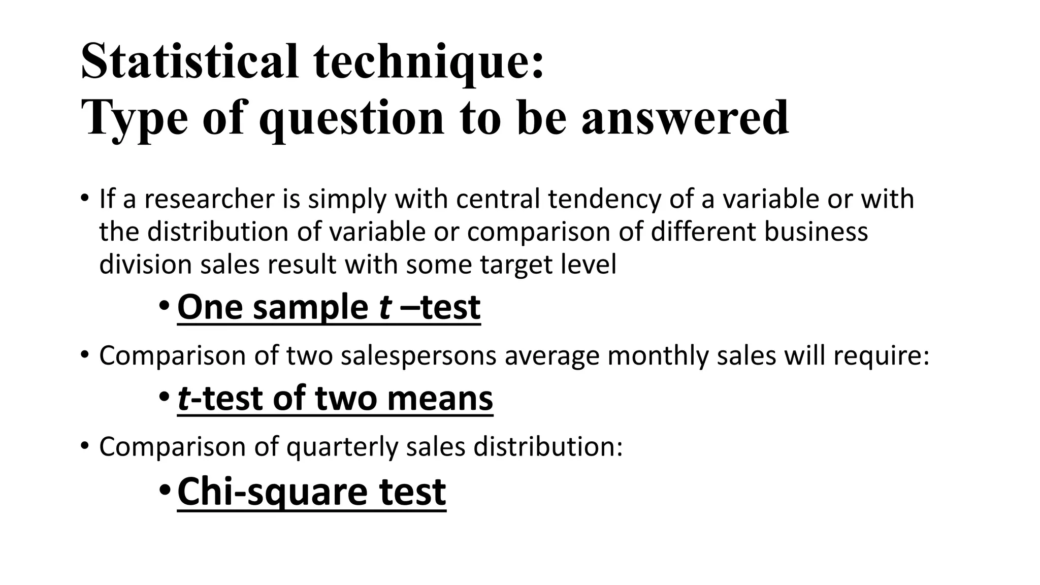
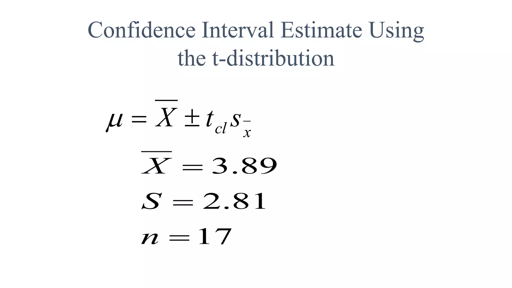
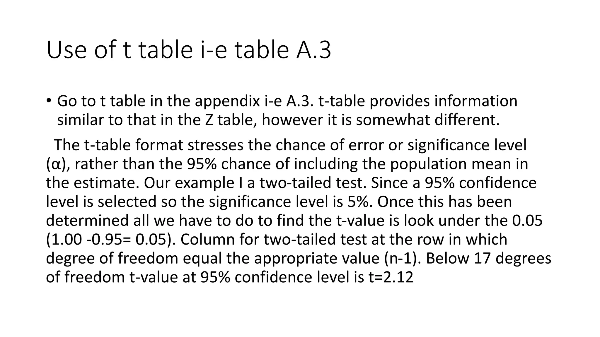
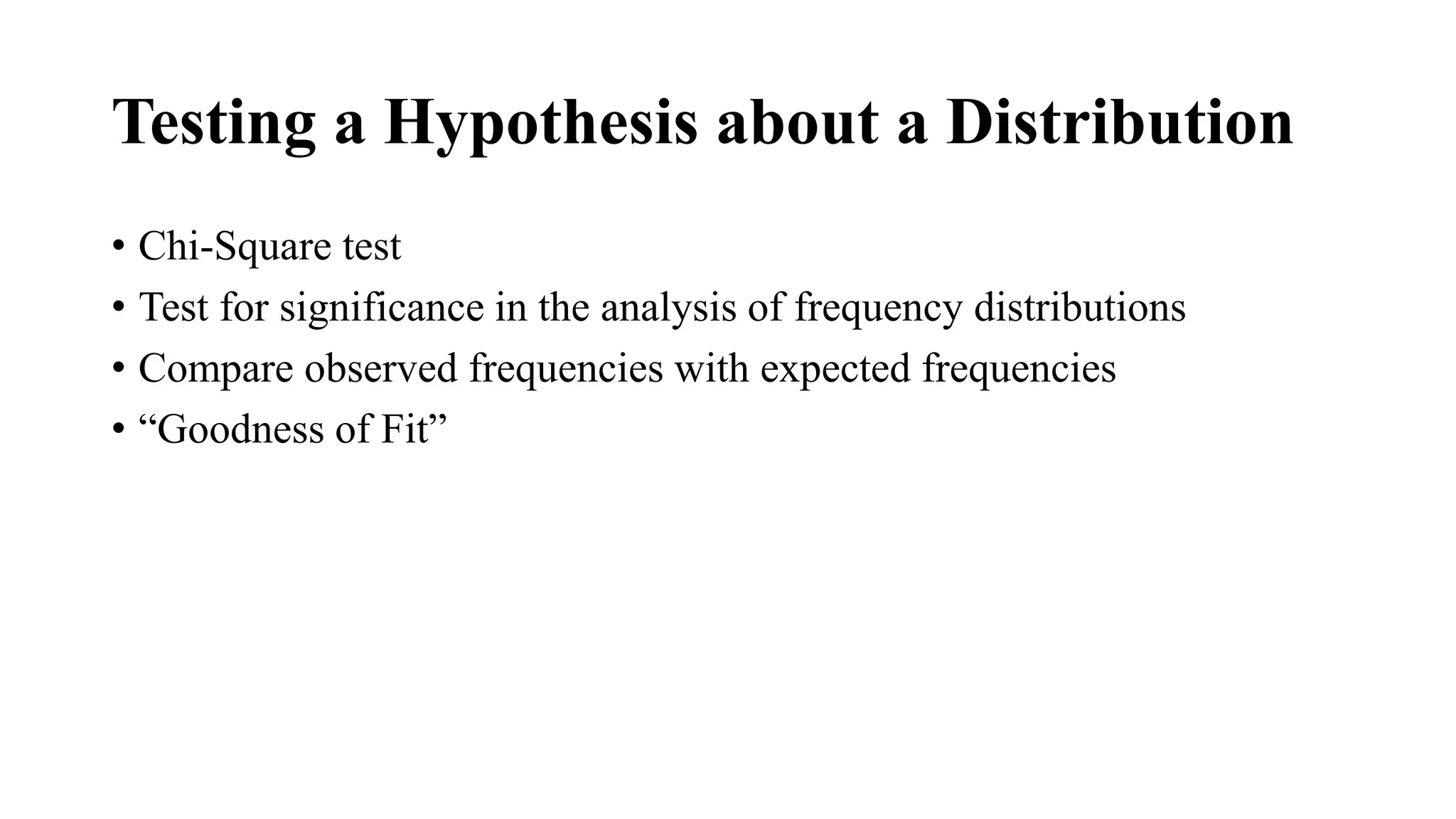
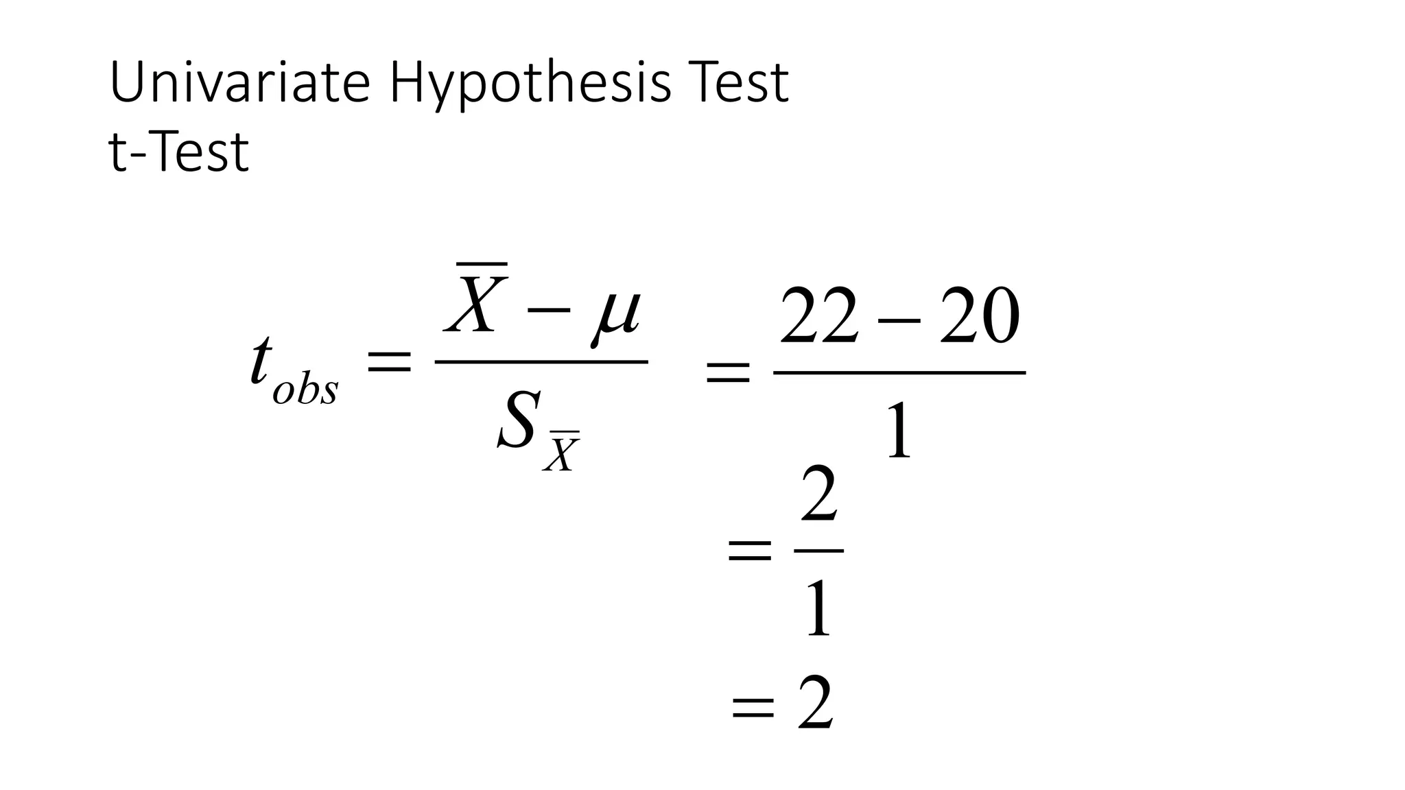
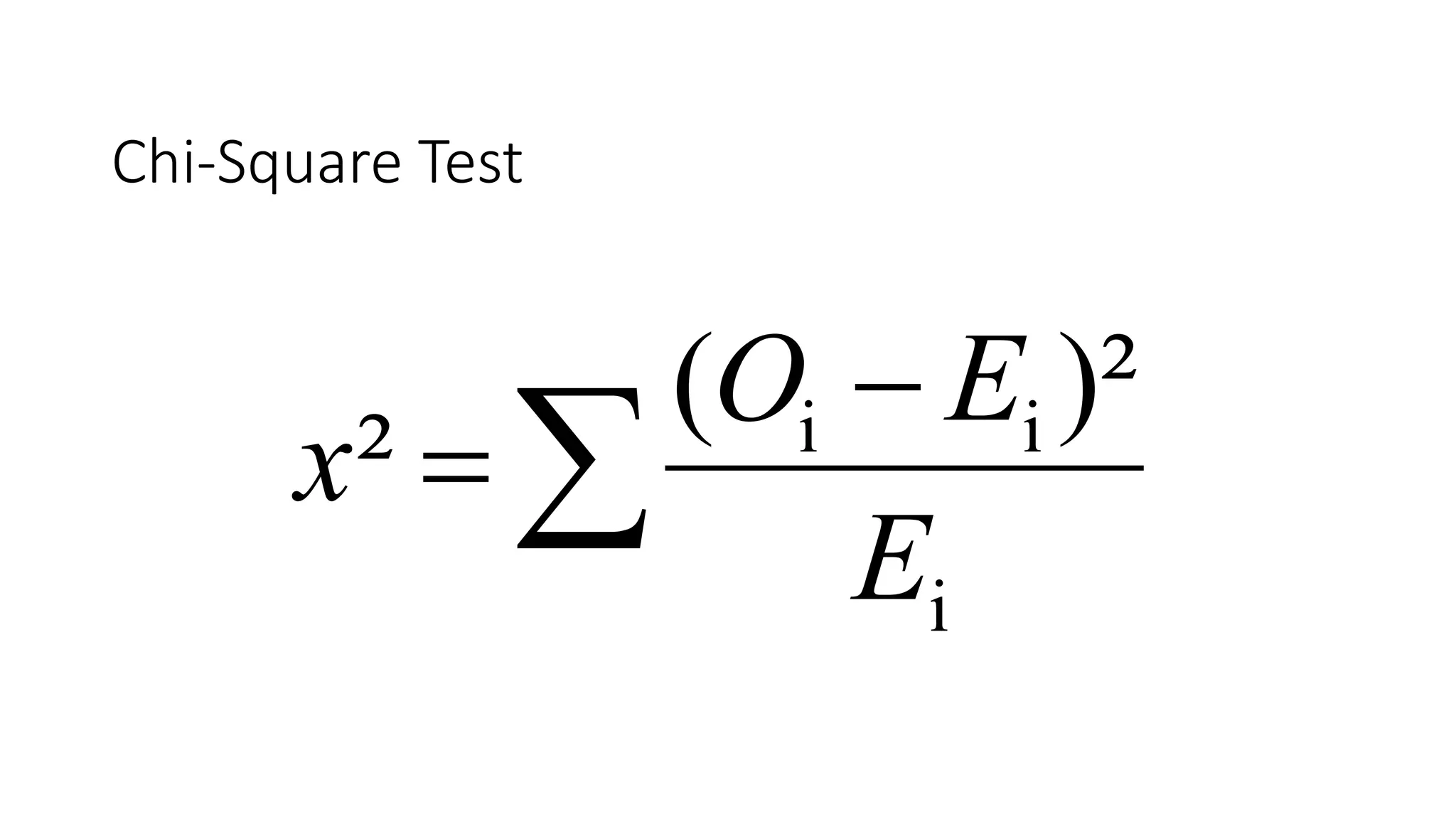
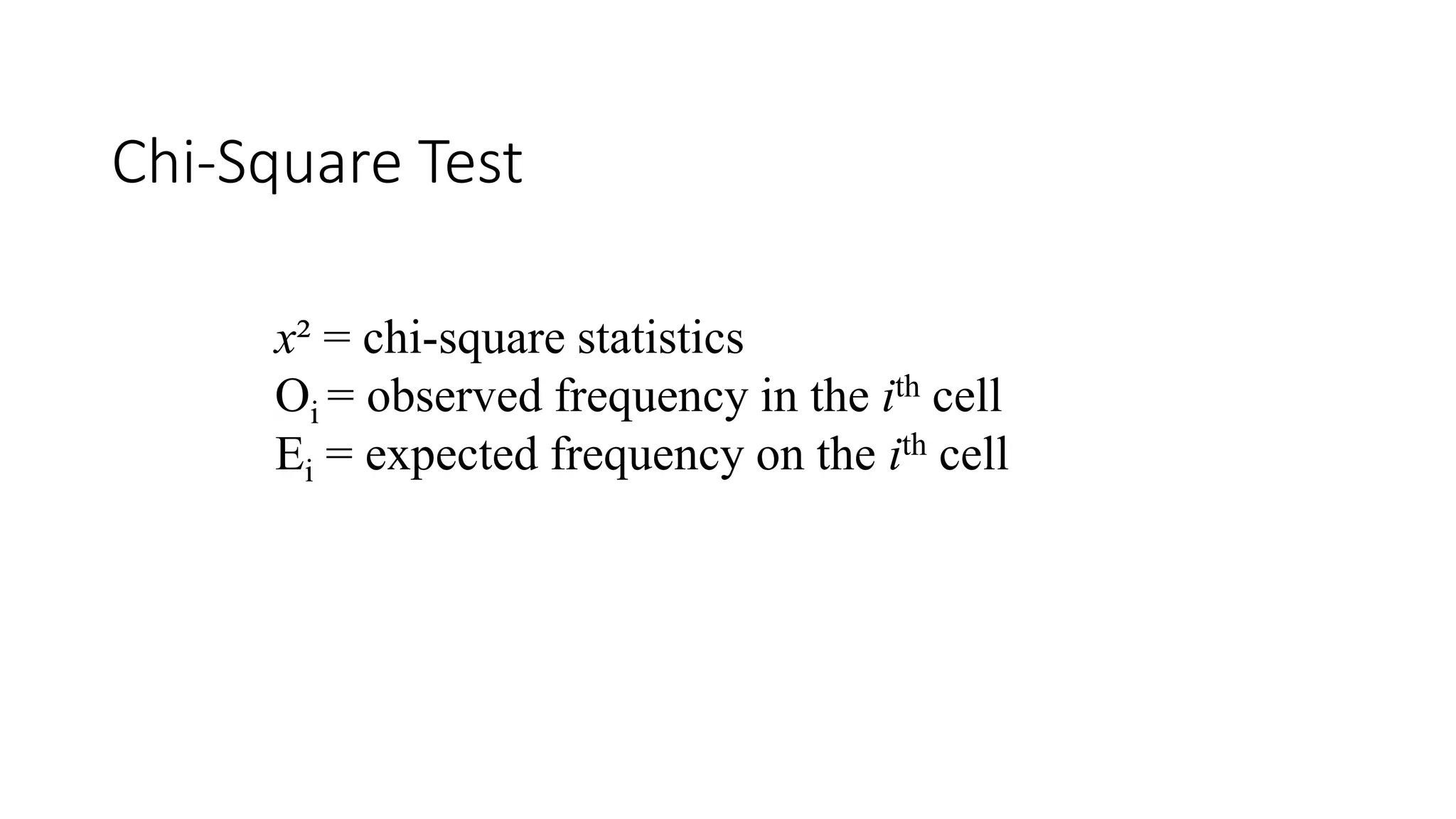
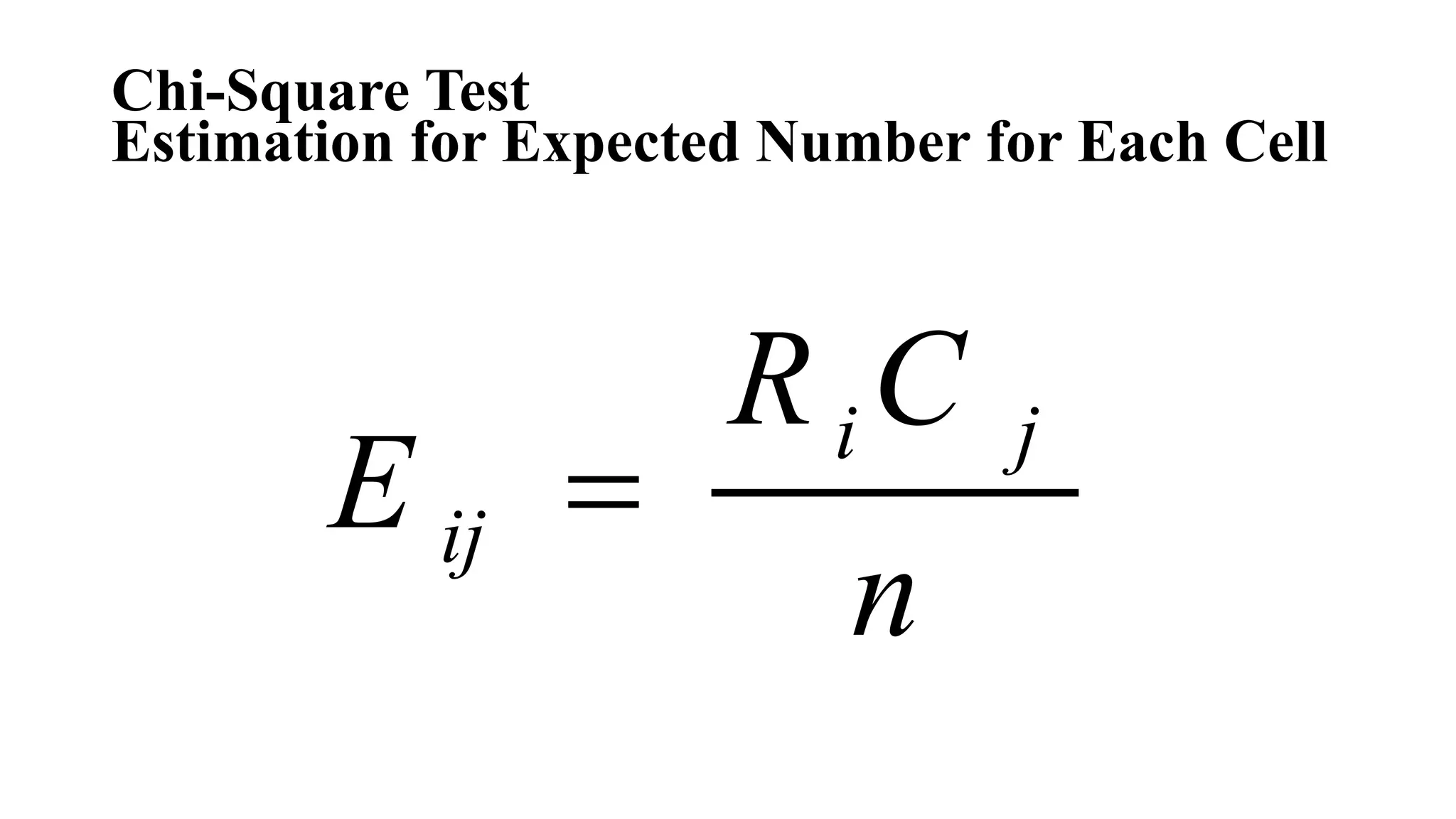
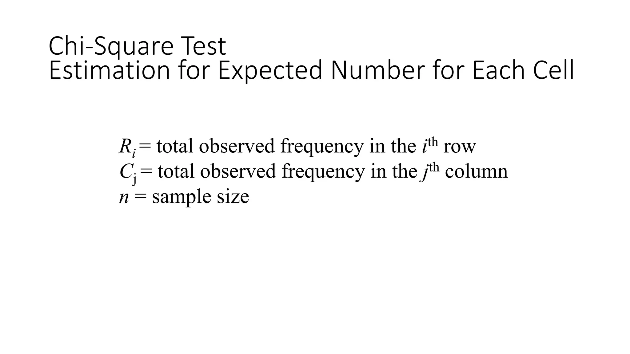
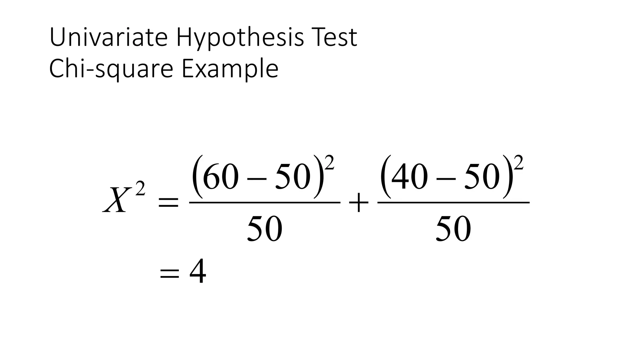
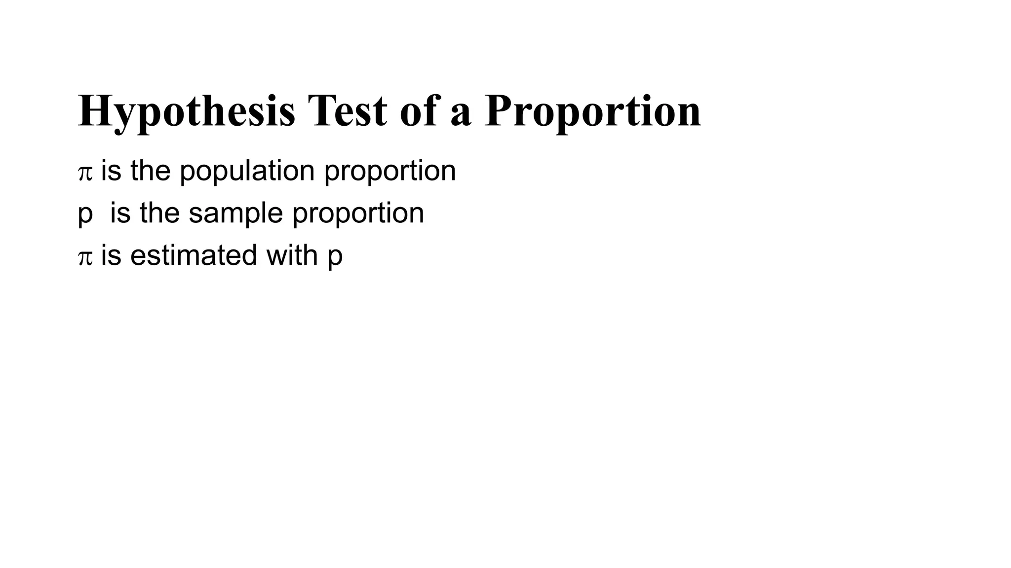
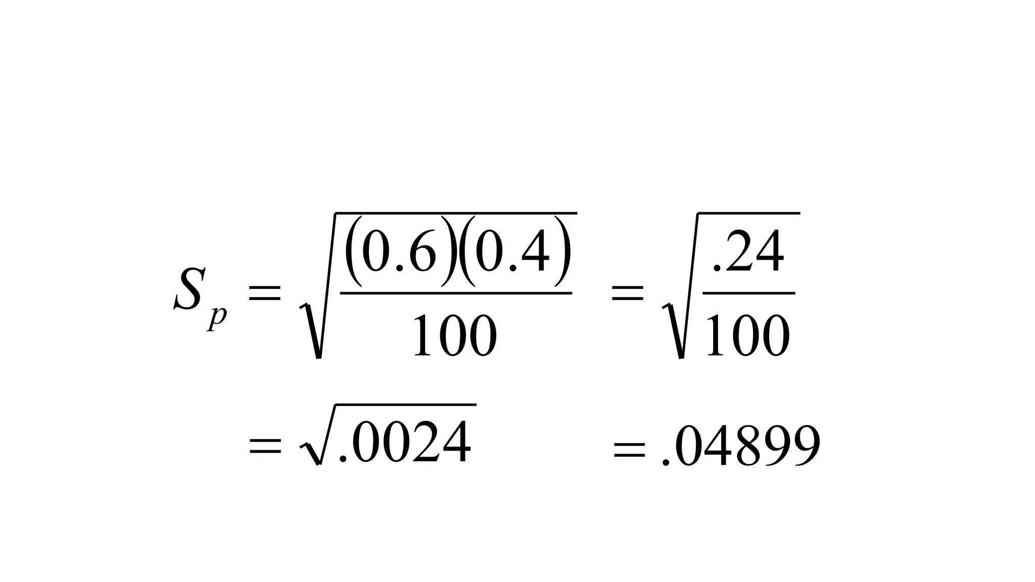
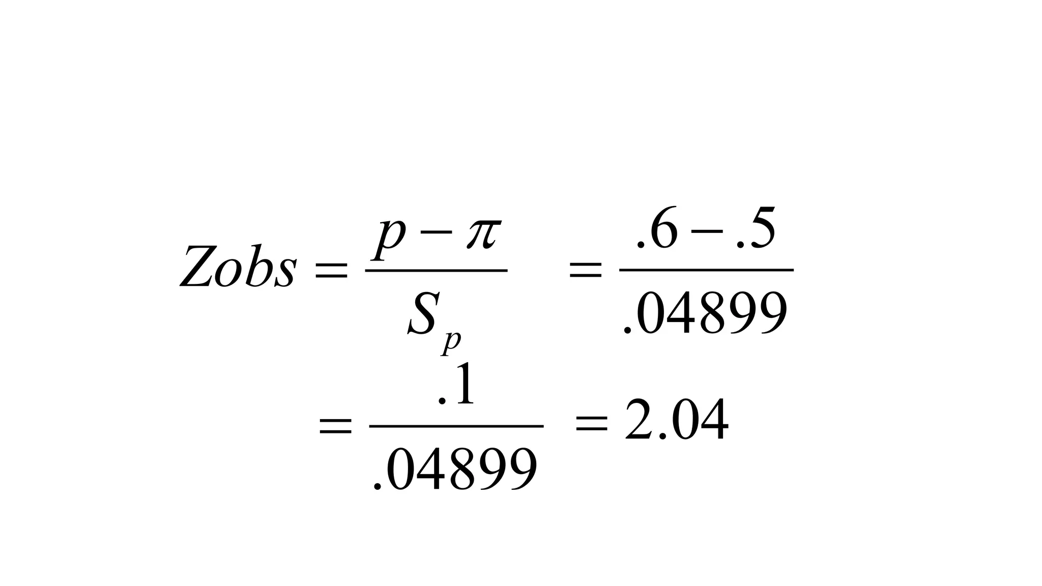
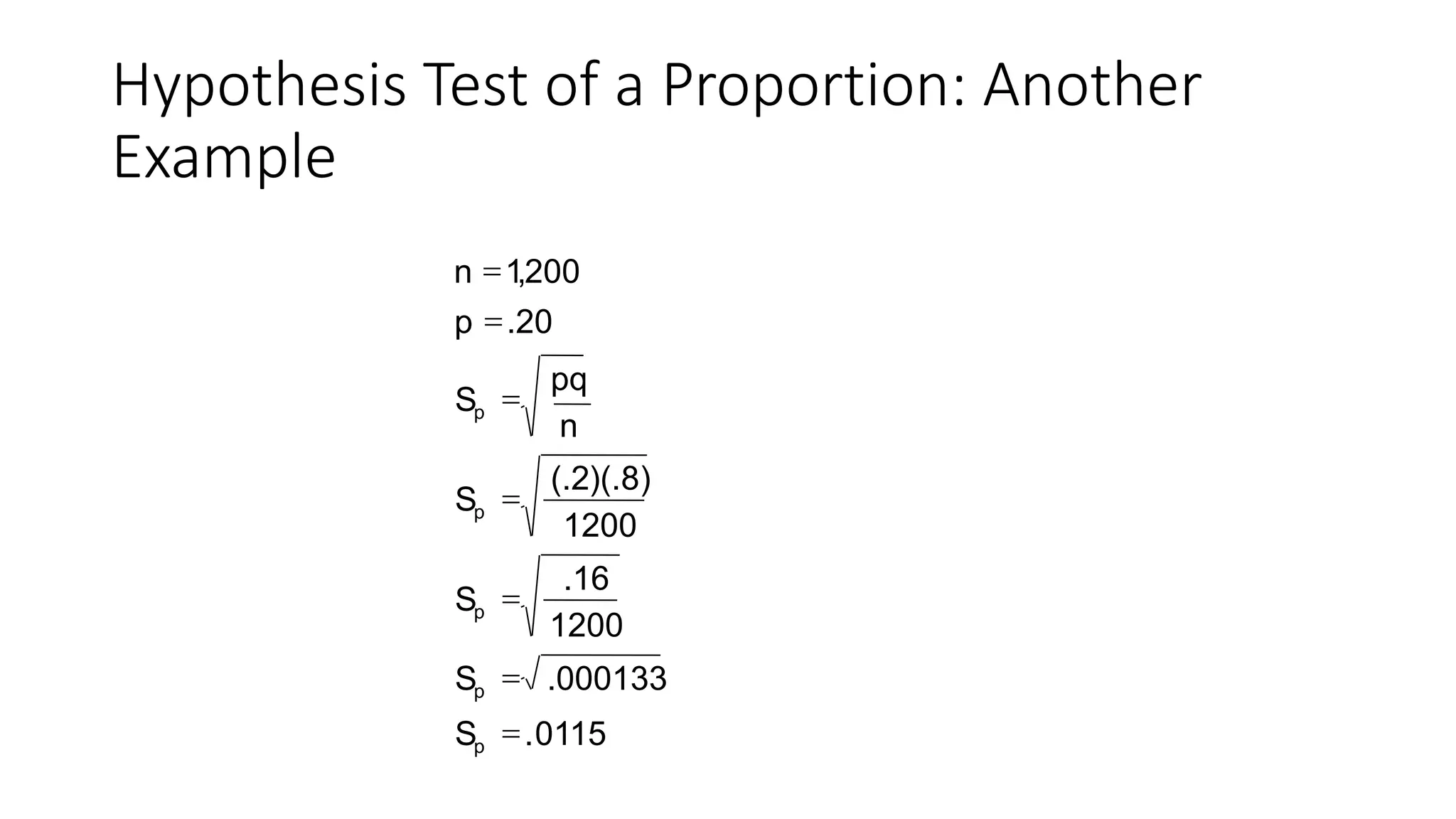
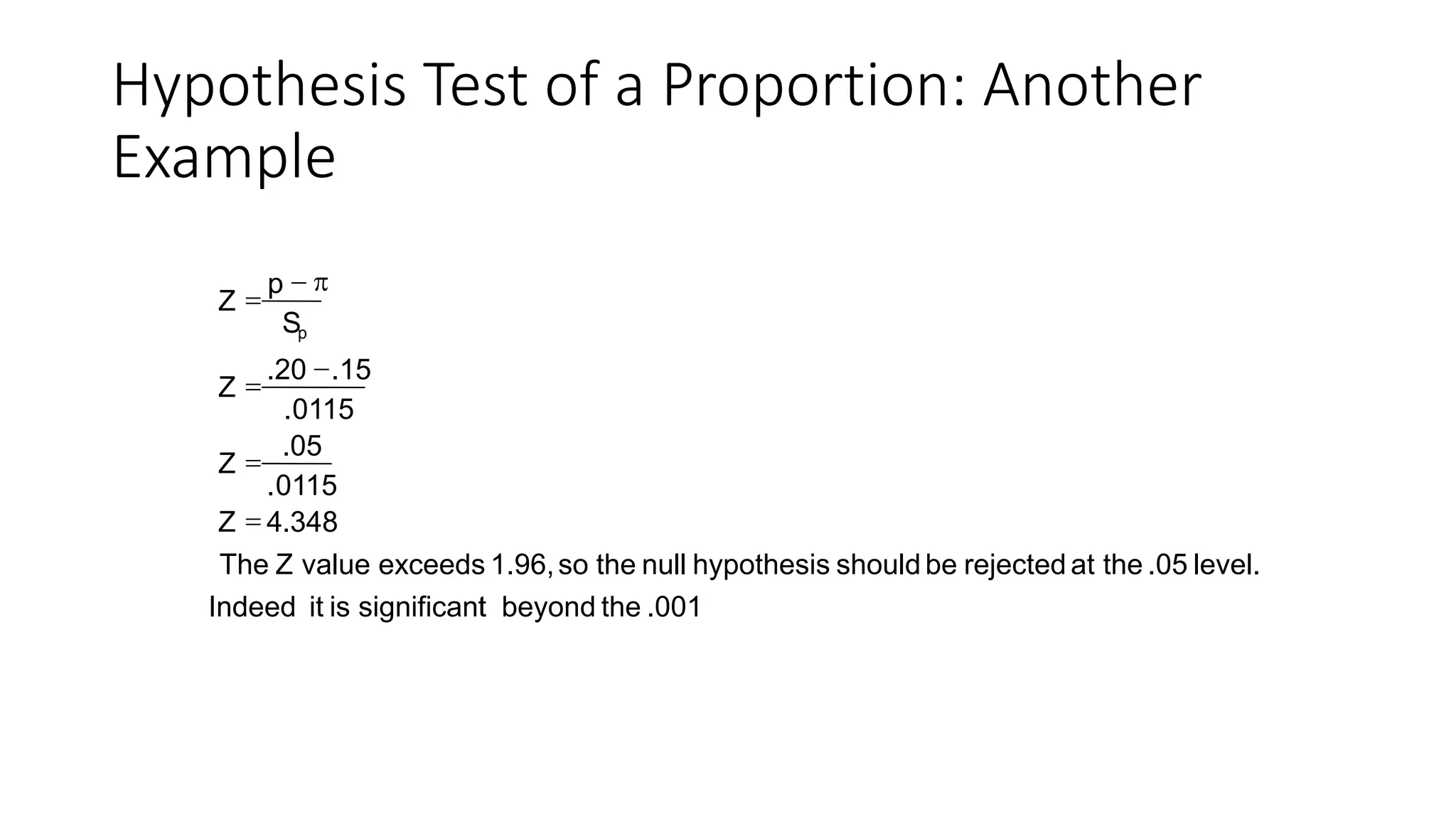
- Common statistical tests like z-test, t-test, chi-square test, and tests of proportions
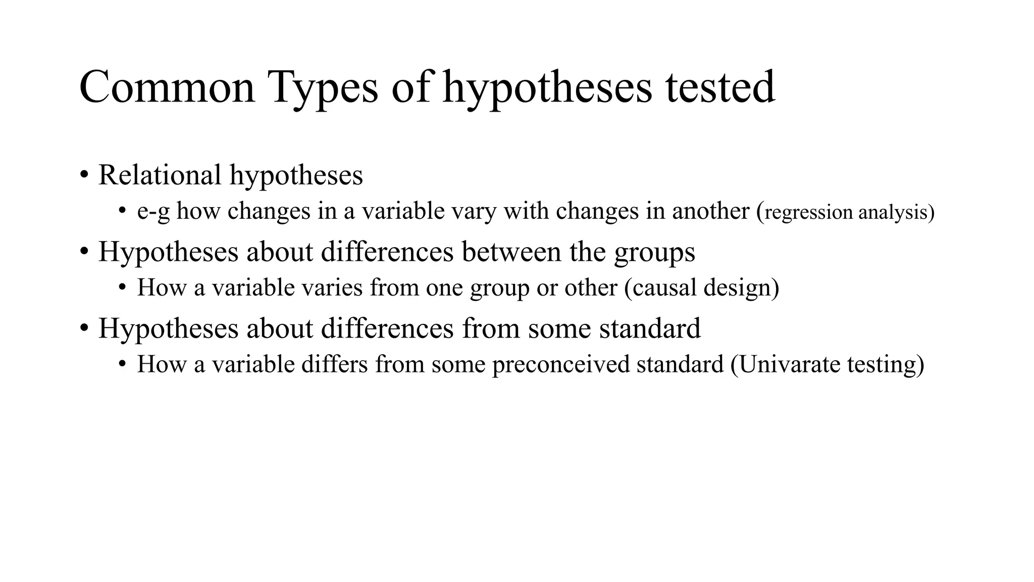
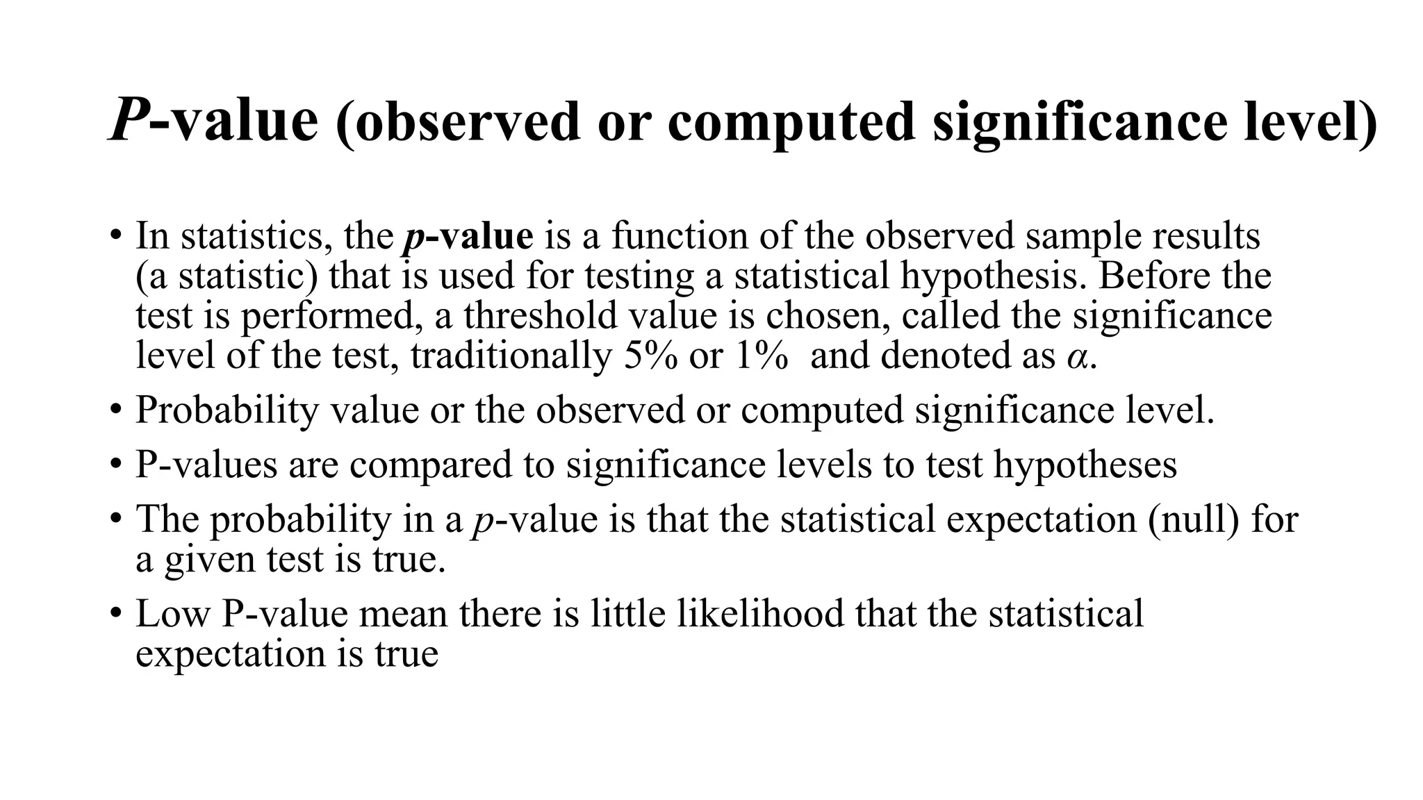
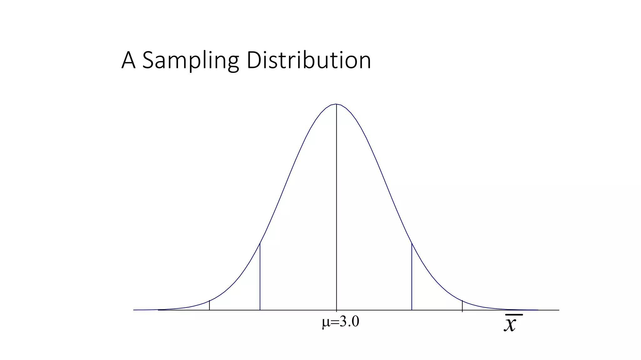
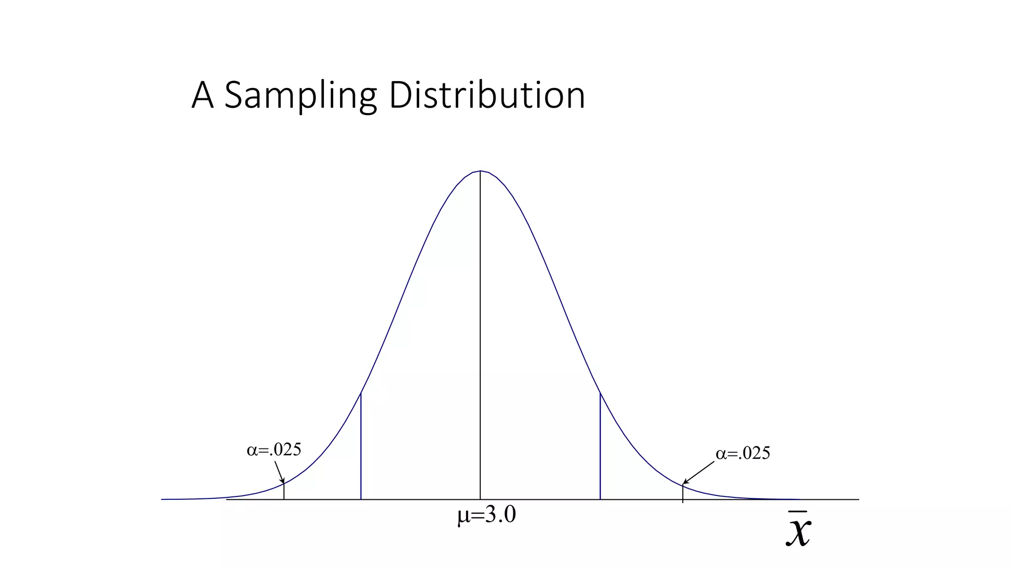
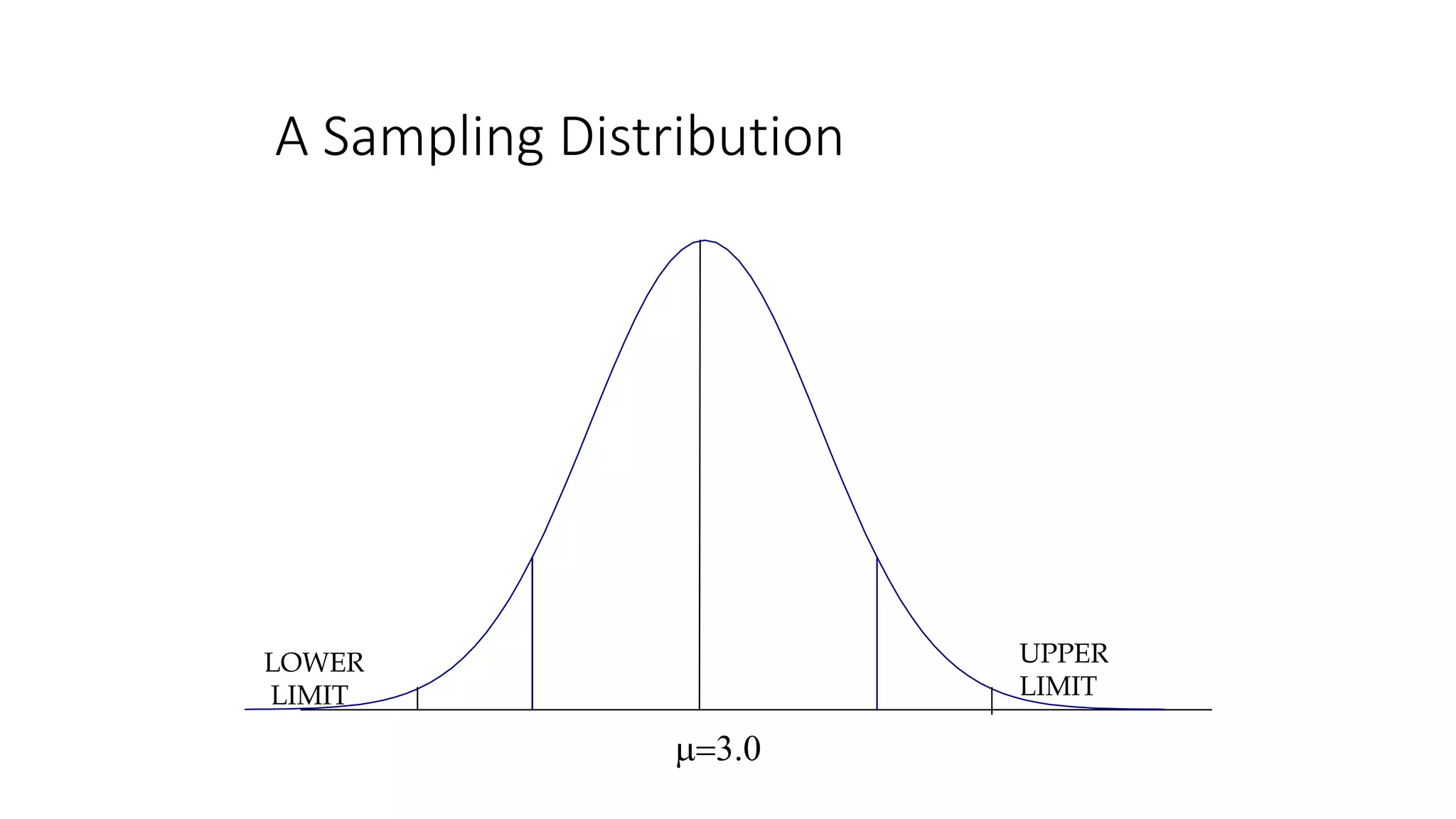
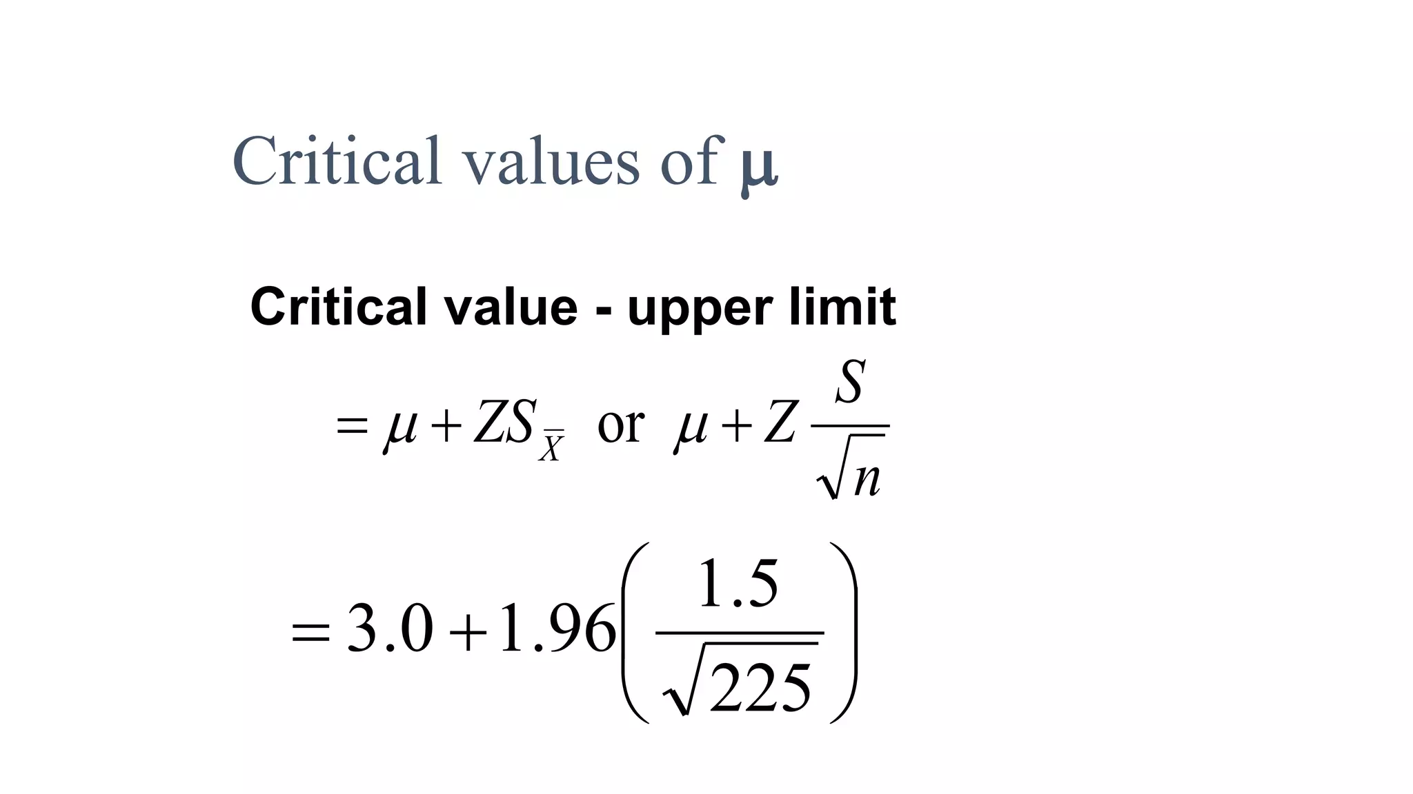
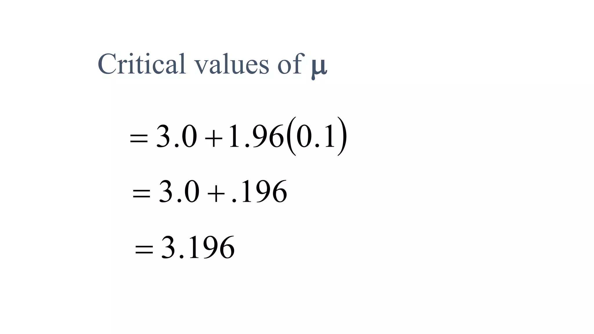
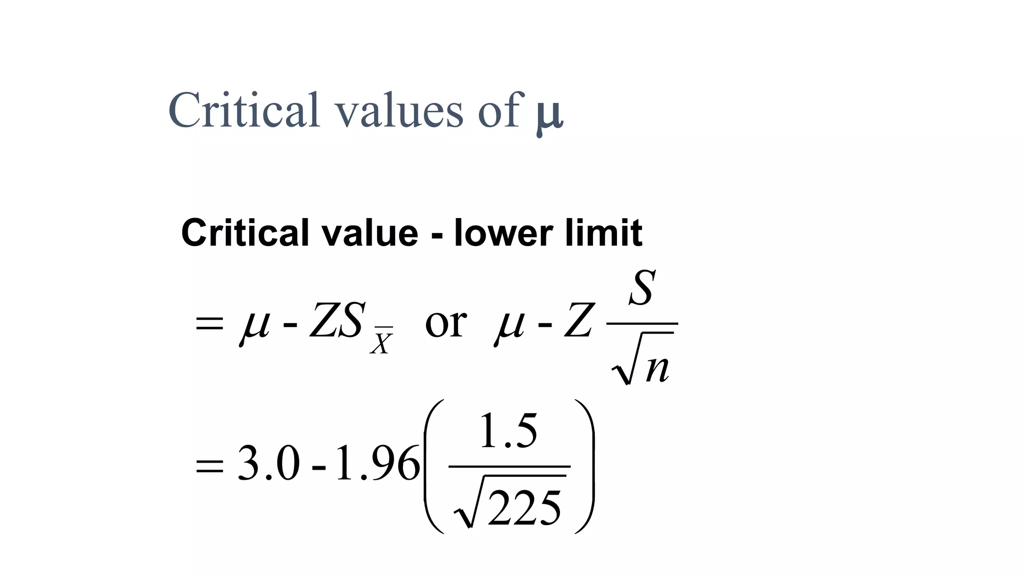
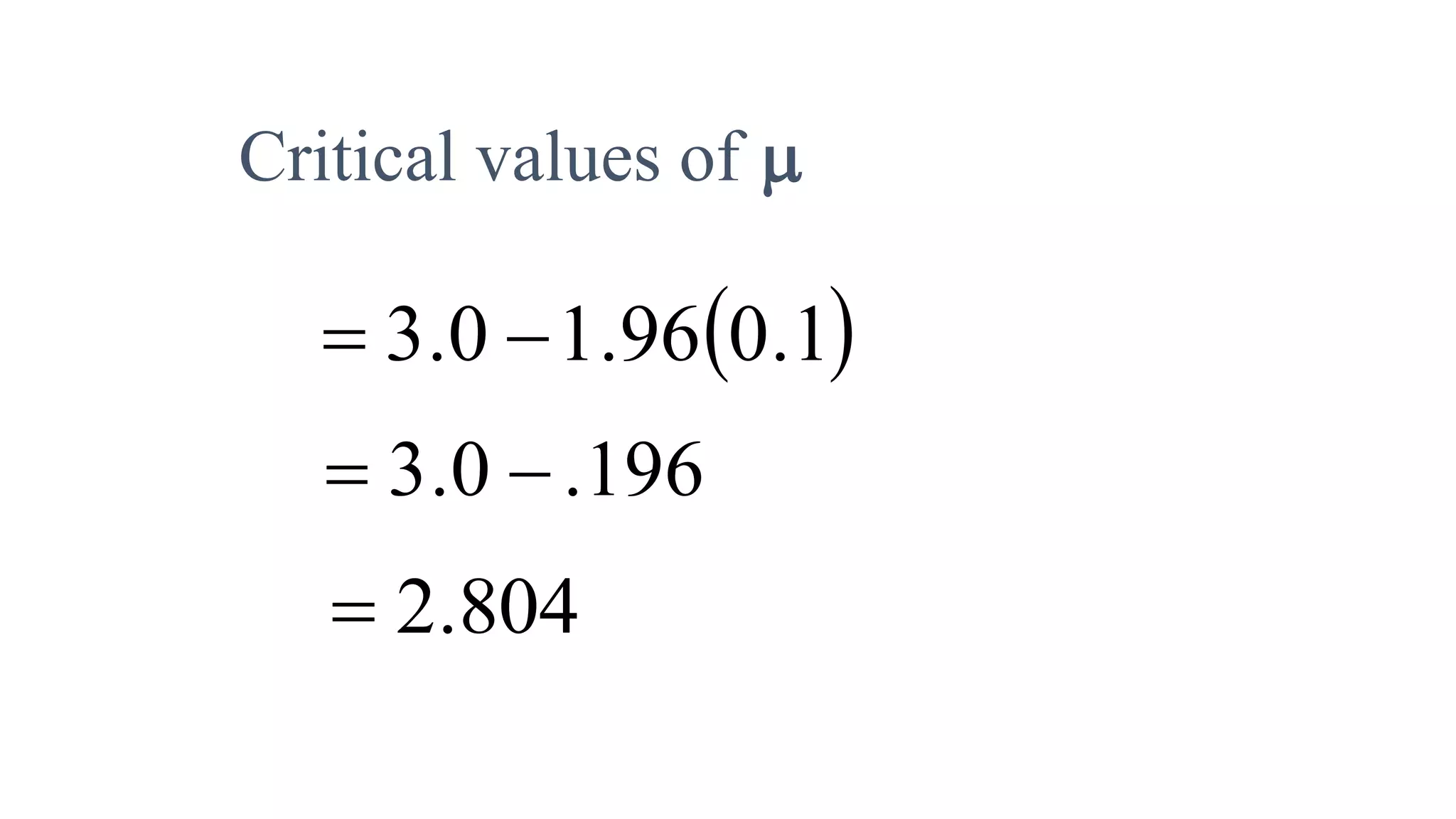
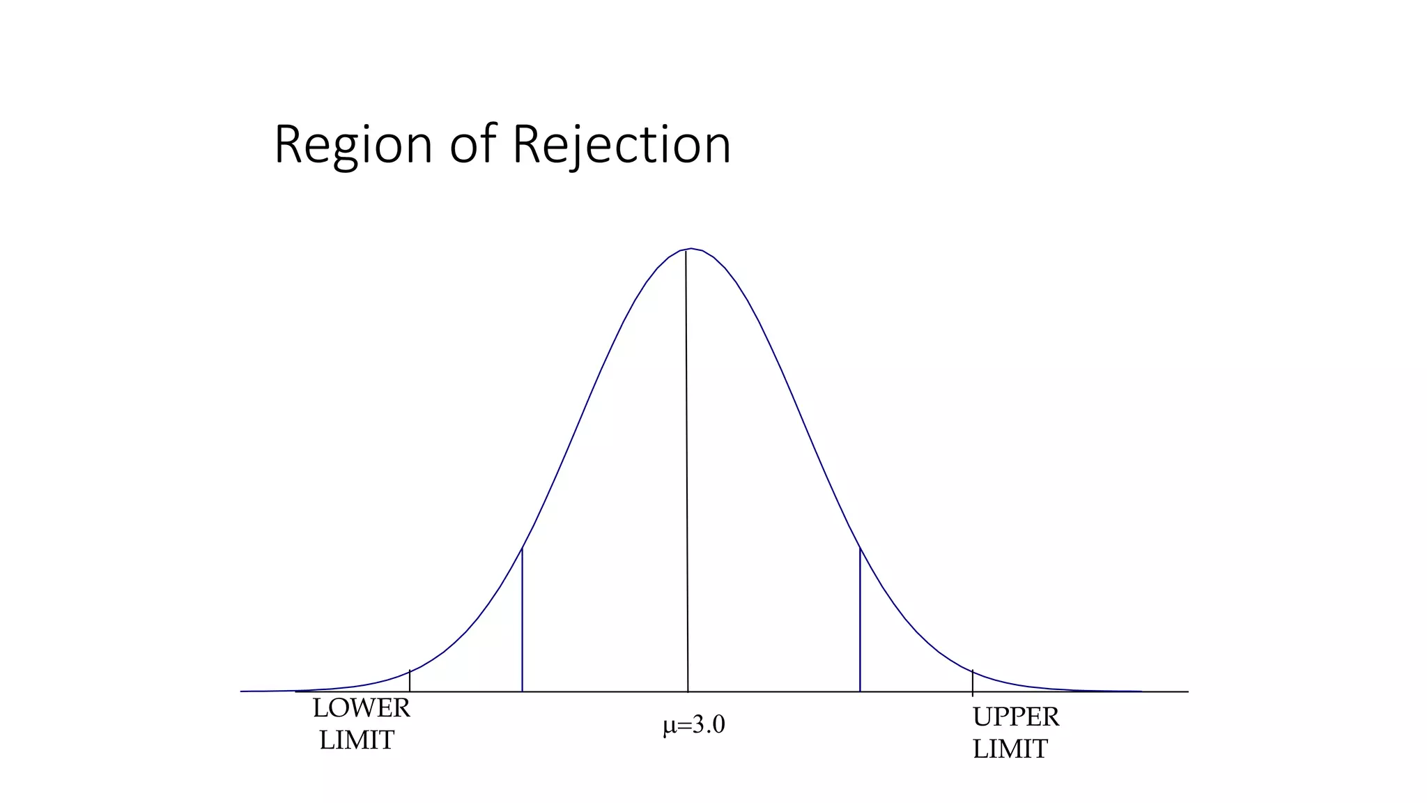
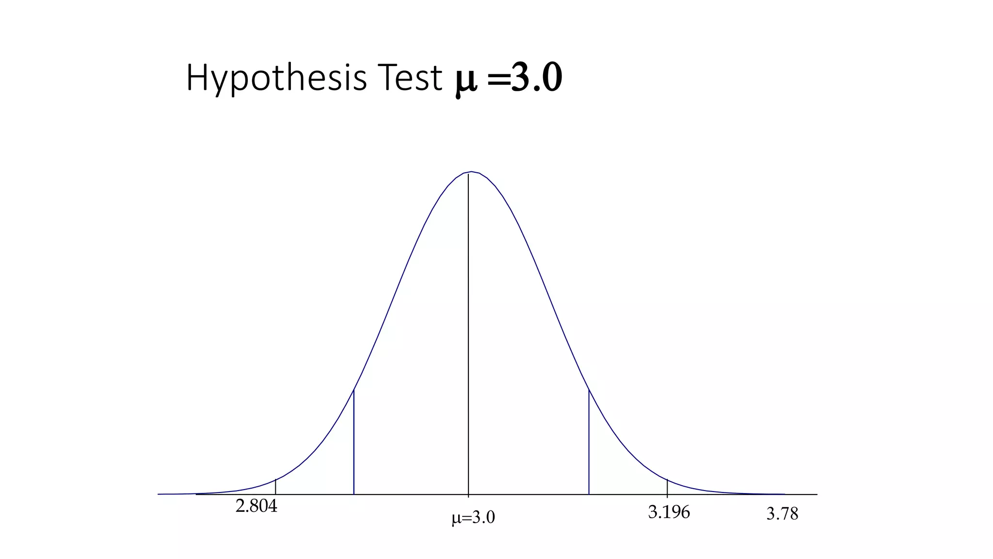
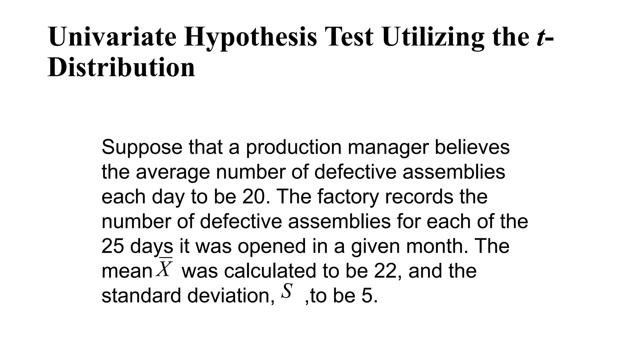
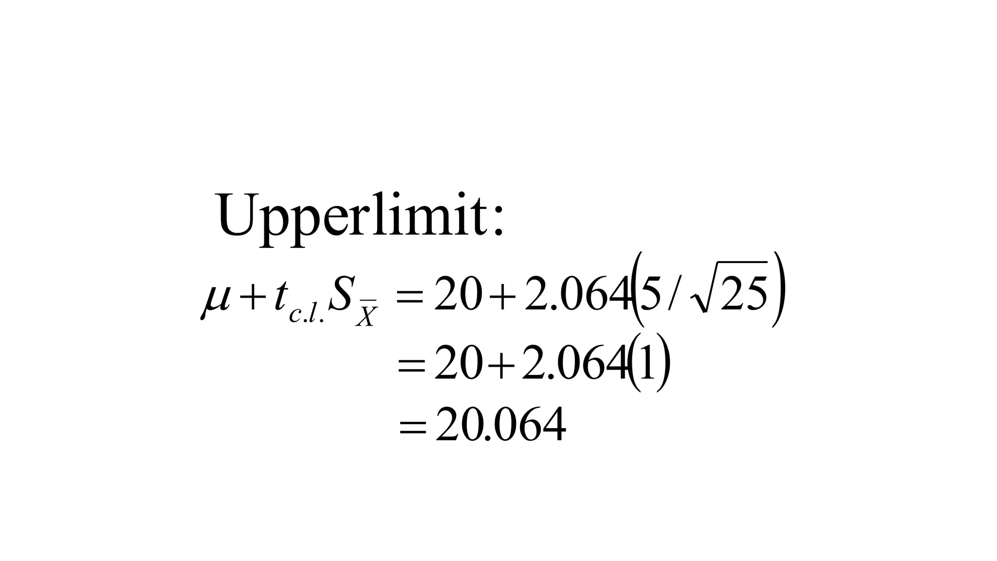
- Key steps in hypothesis testing like defining the hypotheses, determining significance levels, calculating test statistics, and making conclusions
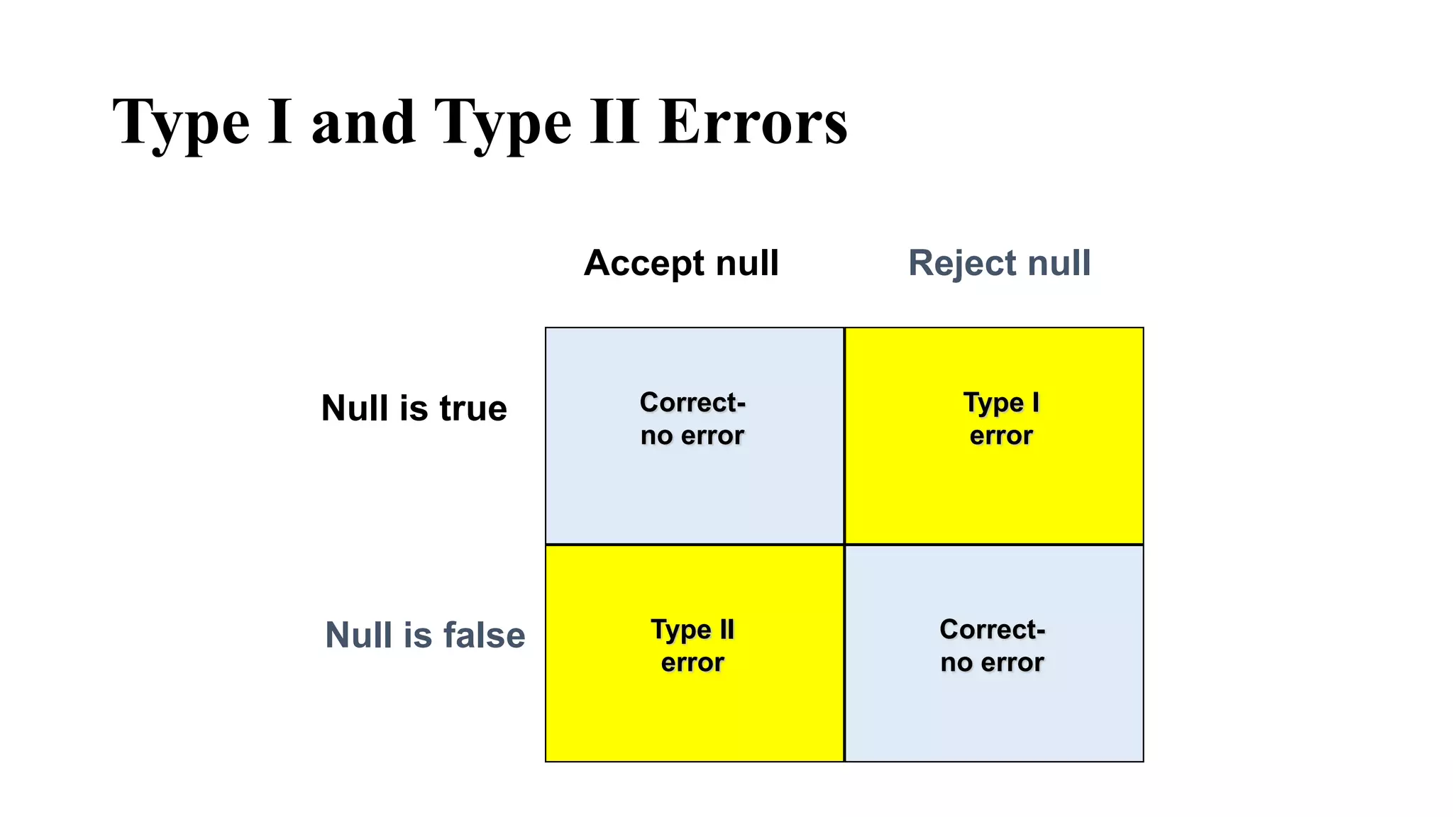
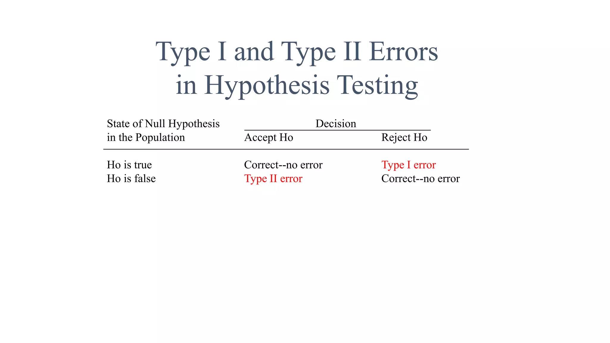
- Types I and II errors that can occur in hypothesis testing
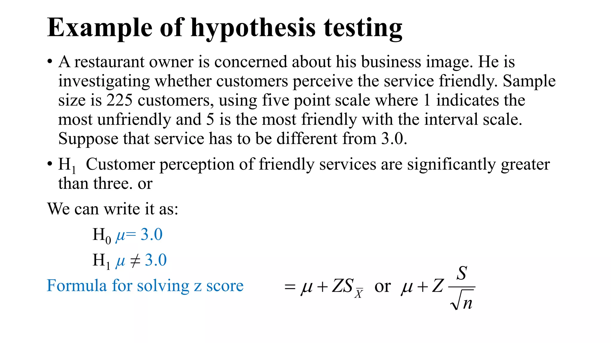
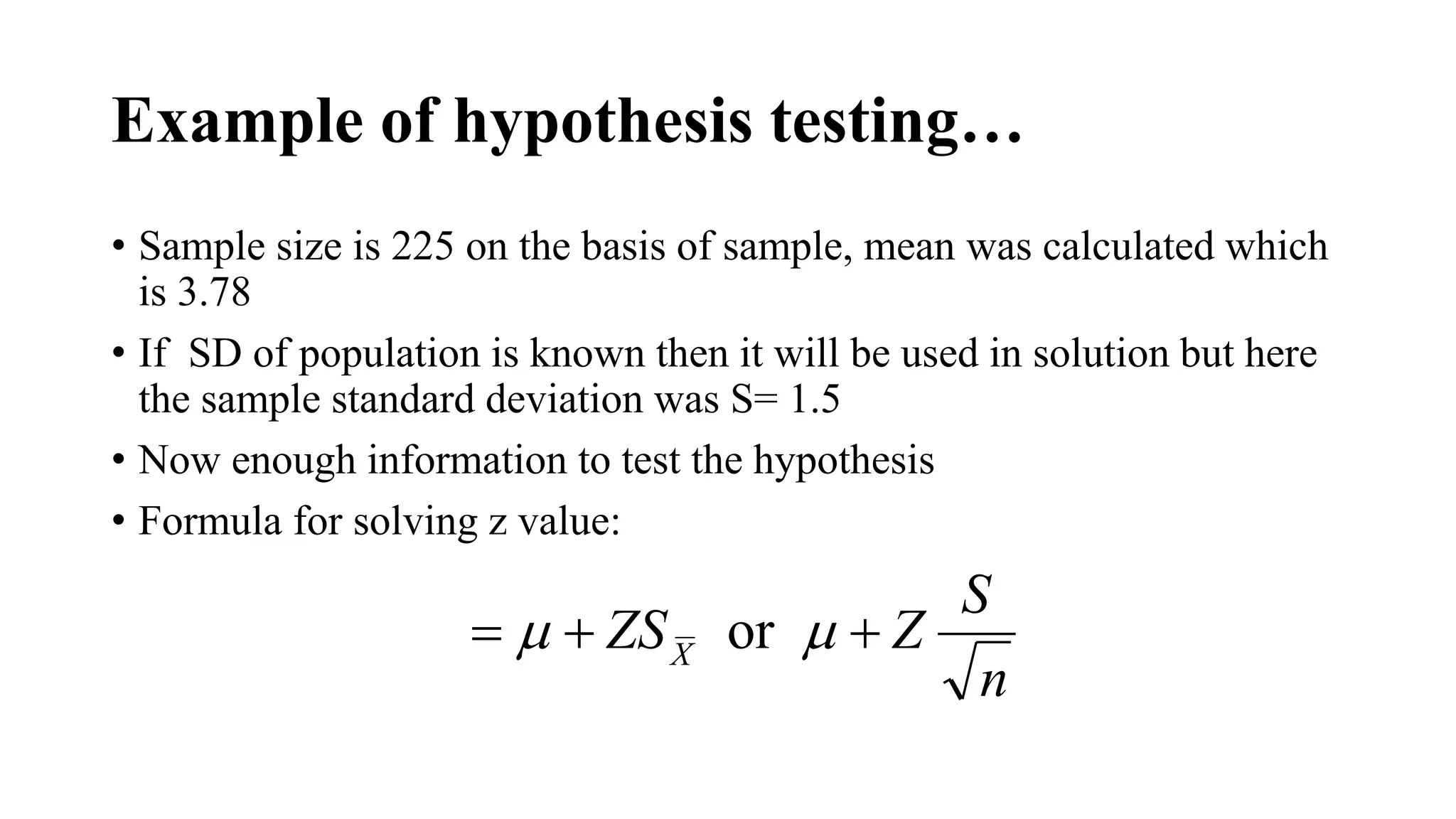
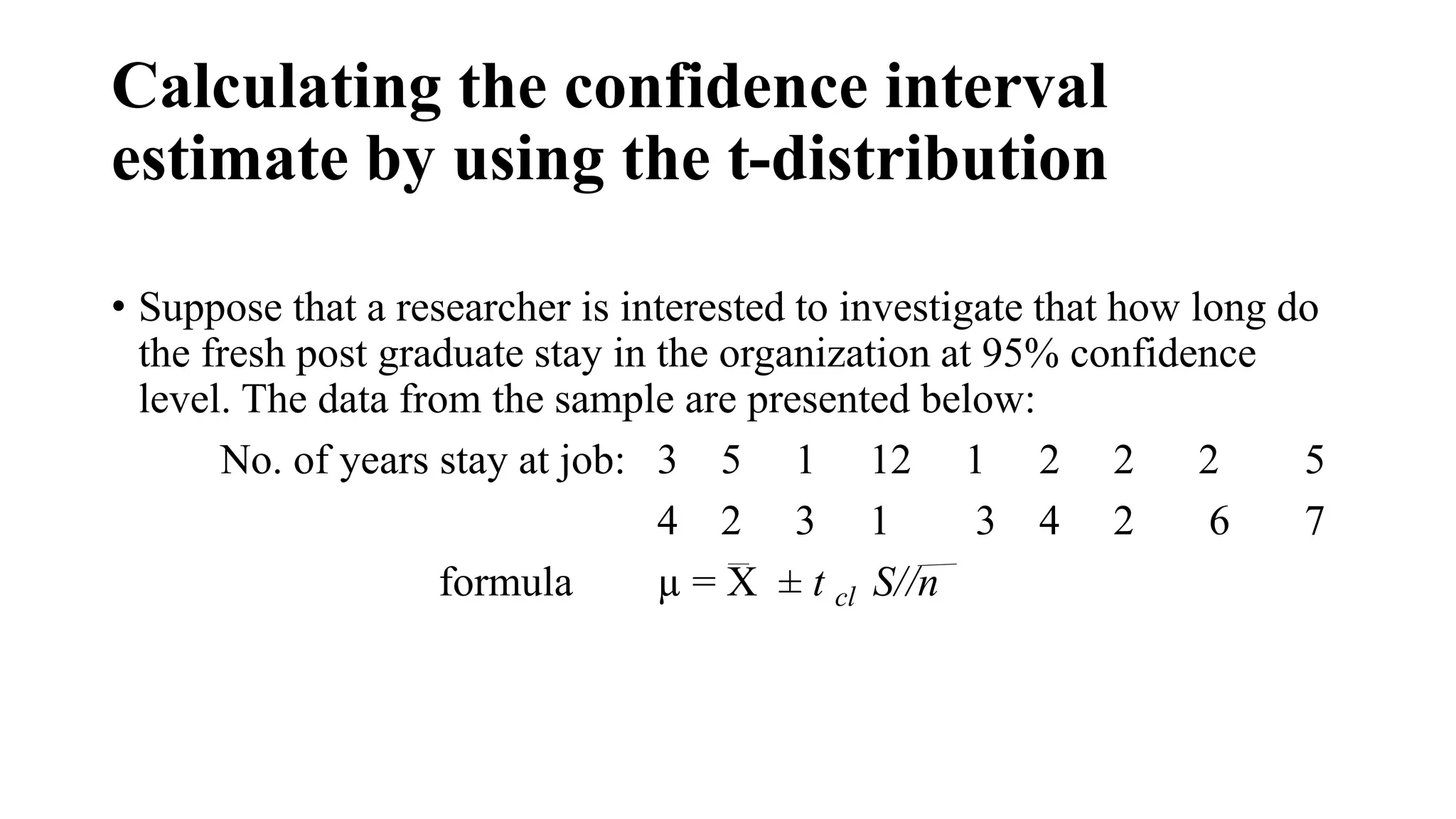
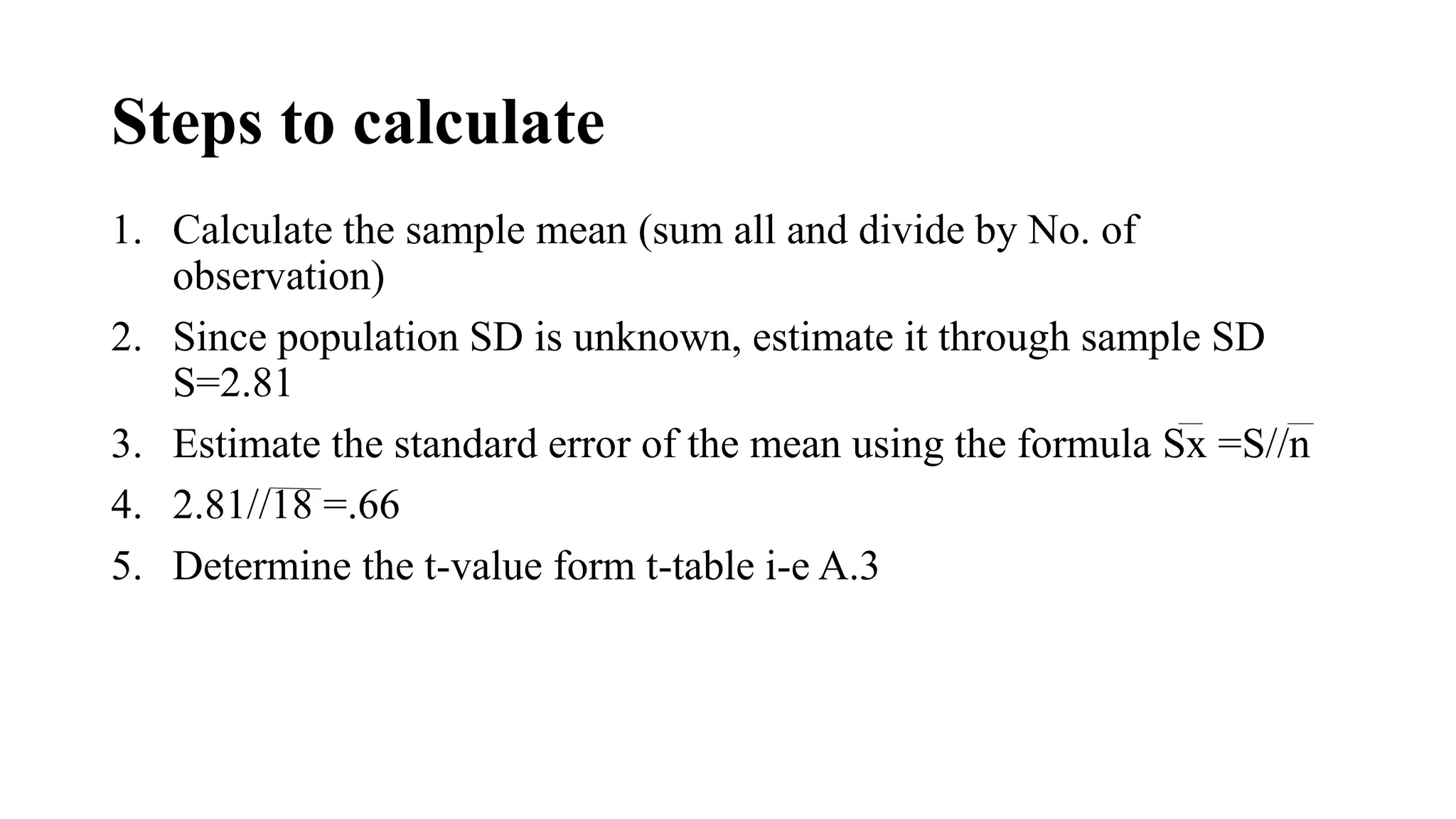
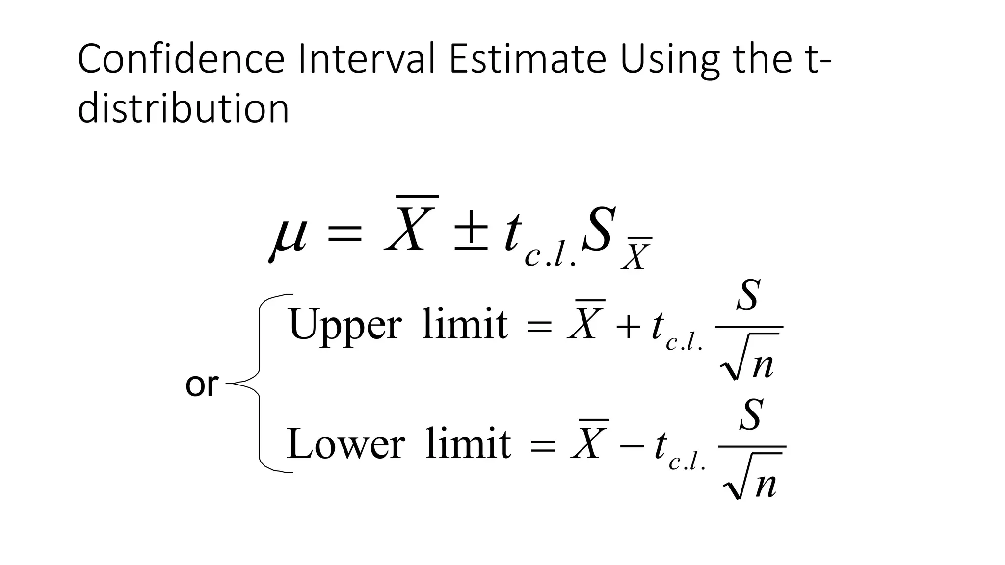
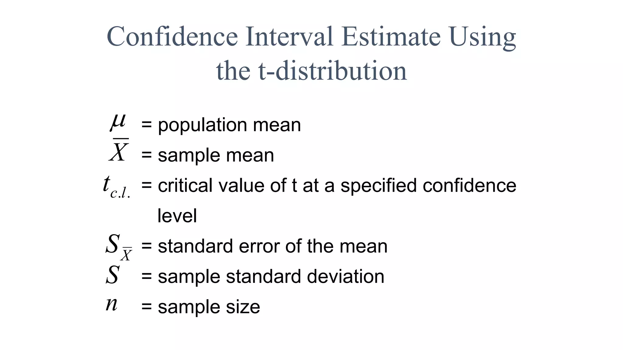
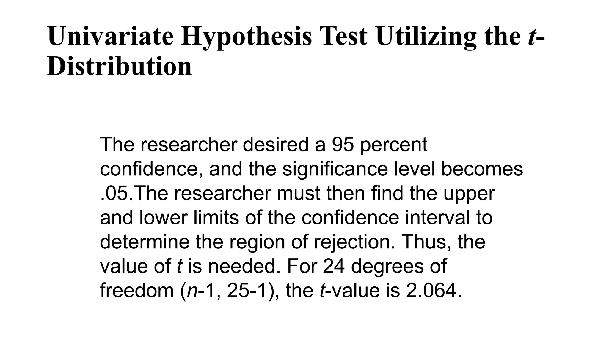
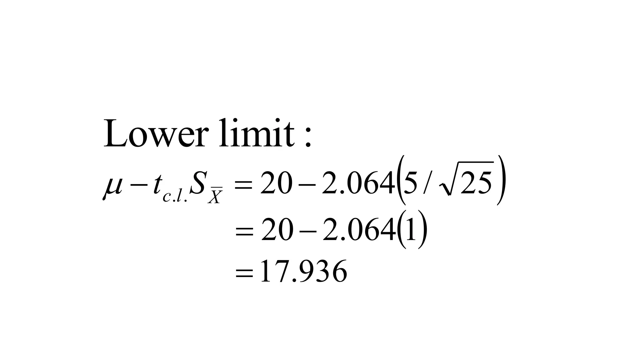
Examples are provided to demonstrate how to set up and conduct hypothesis tests using z-test, t-test, chi-square test, and test of proportions.