Downloaded 175 times


1) Continuous random variables have cumulative distribution functions (CDFs) that are continuous functions of the variable. They can have probability density functions (pdfs) that define their distributions. 2) Exponential distributions describe systems with memoryless properties where the probability of failure does not depend on past events. They commonly model time between events like packet arrivals. 3) Uniform distributions have constant pdfs across their range, resulting in a linear CDF ramp function. They are commonly used in random number generation.
Introduction to continuous random variables and presentation details.
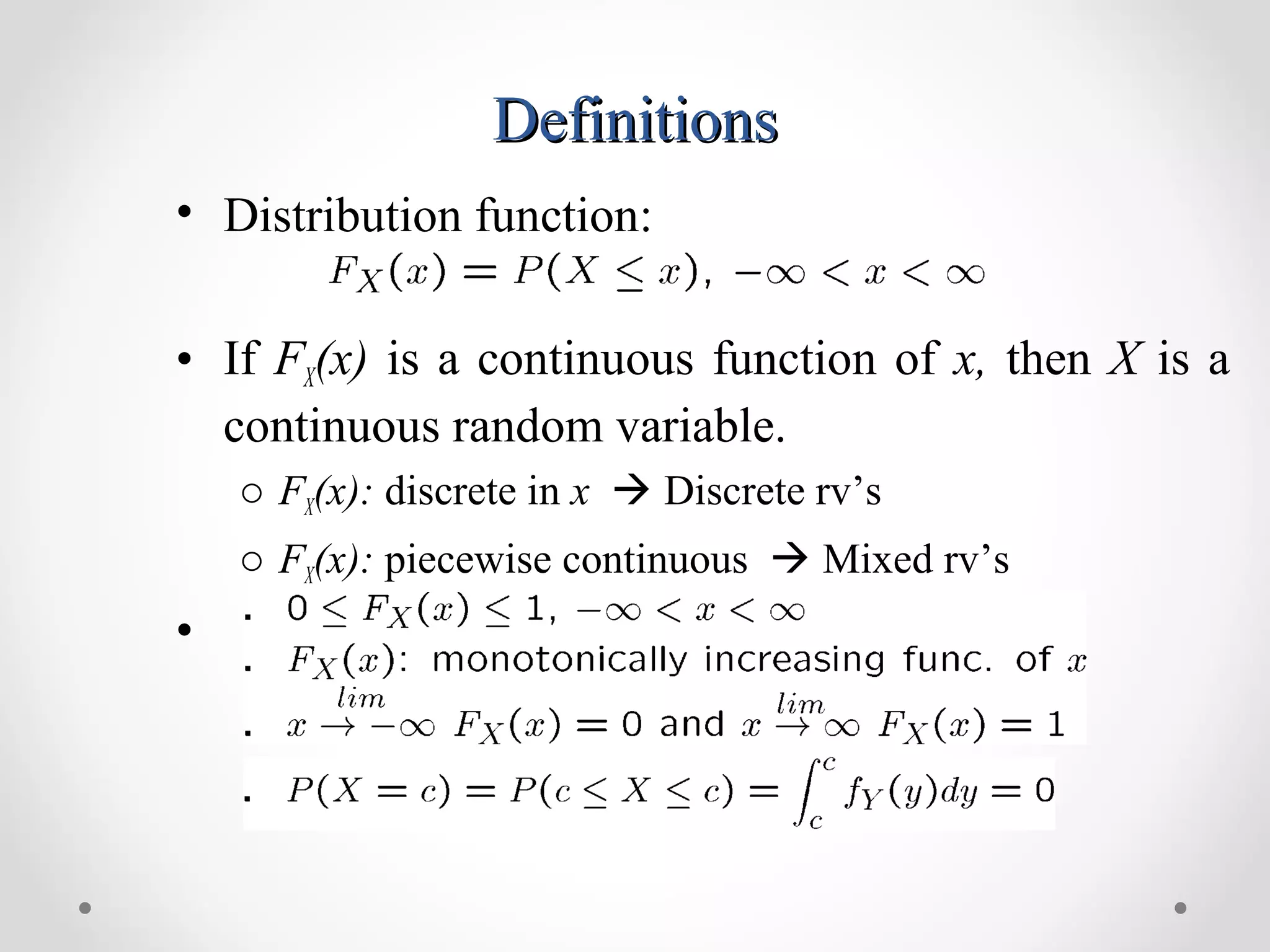
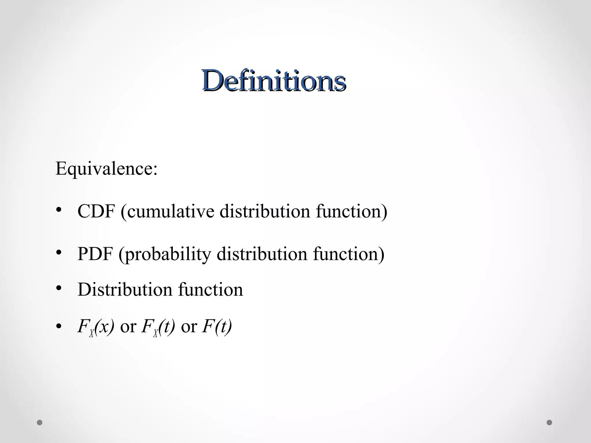
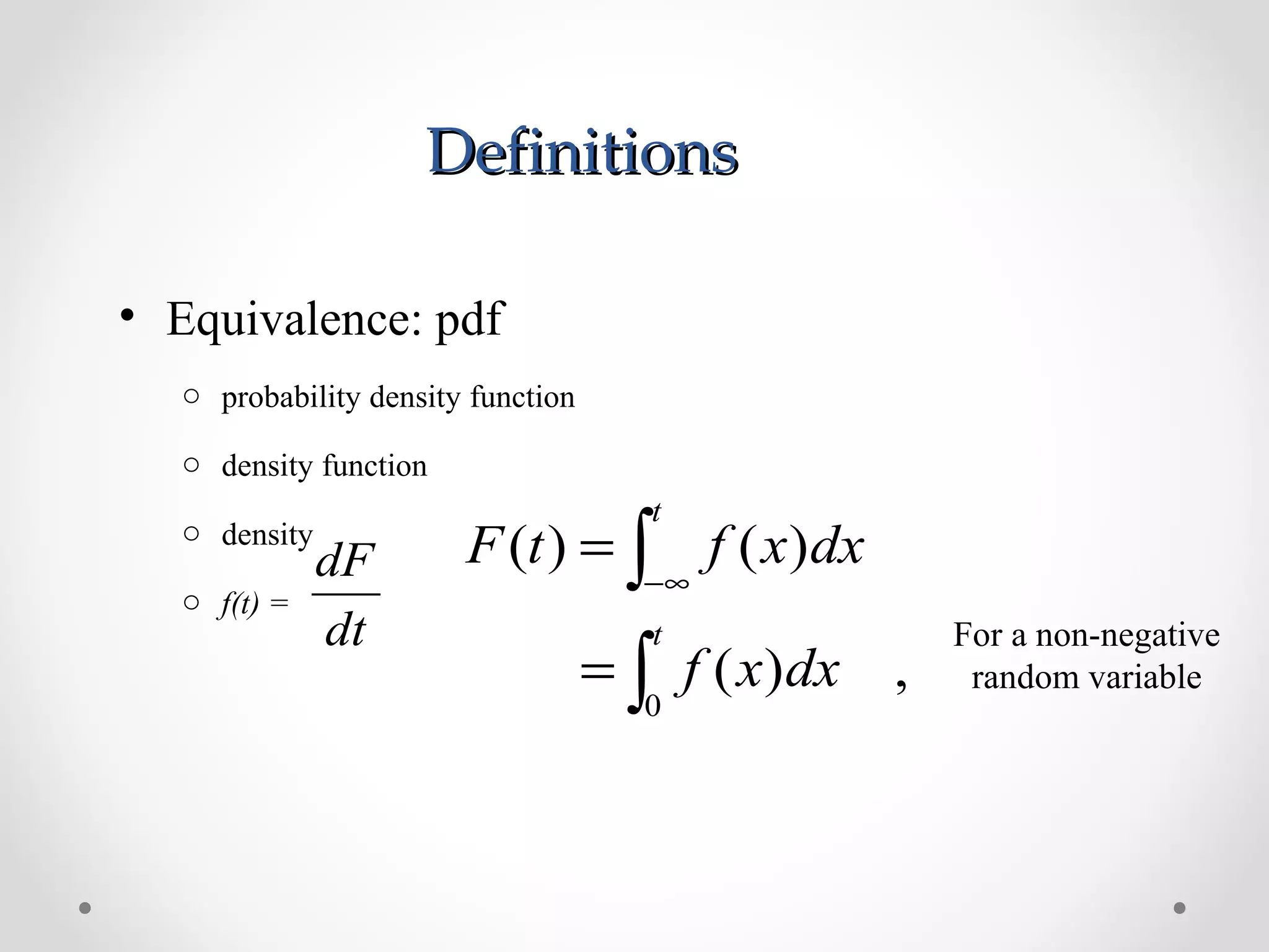
Definition of distribution functions: continuous random variable, CDF, PDF equivalence.
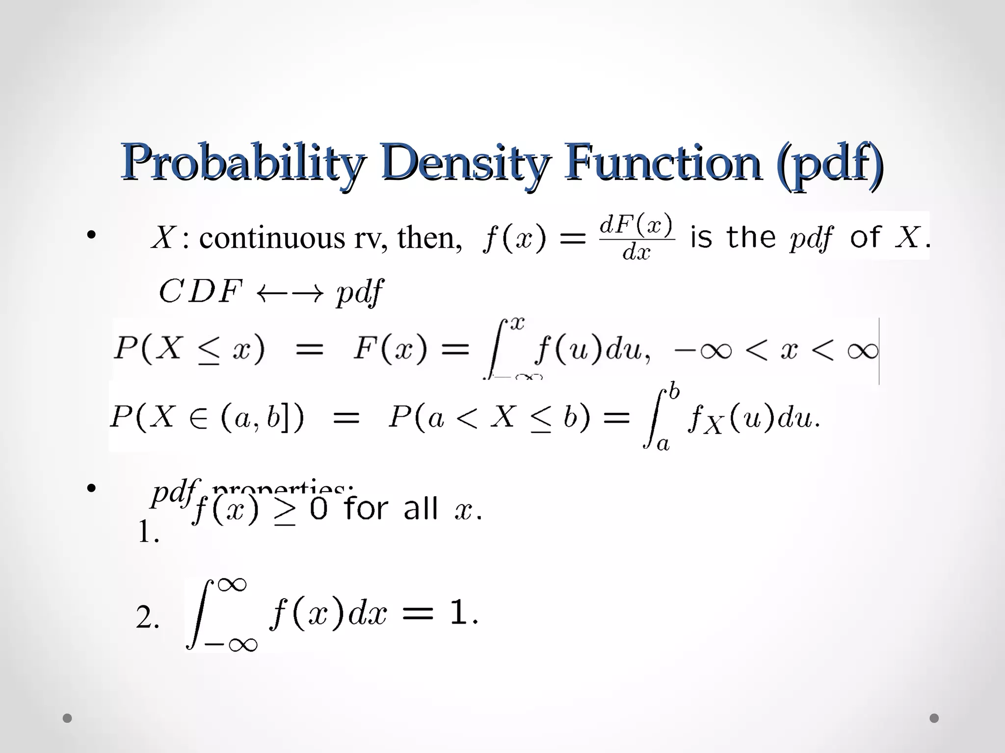
Explains properties of the probability density function (pdf) for continuous random variables.
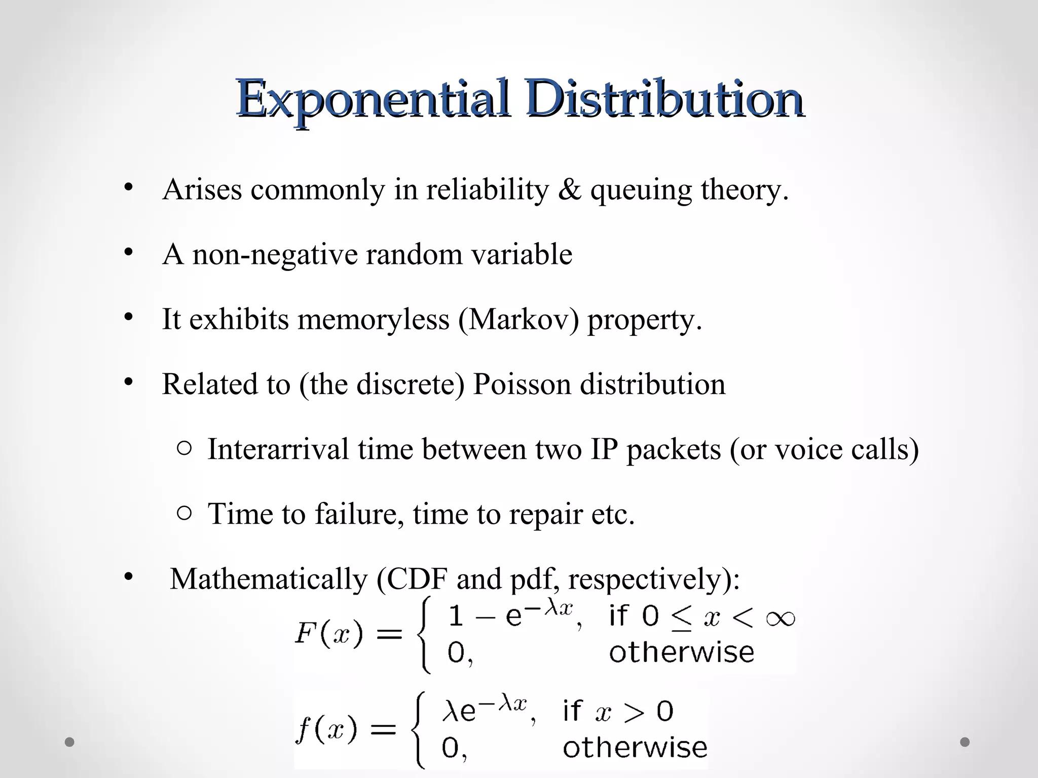
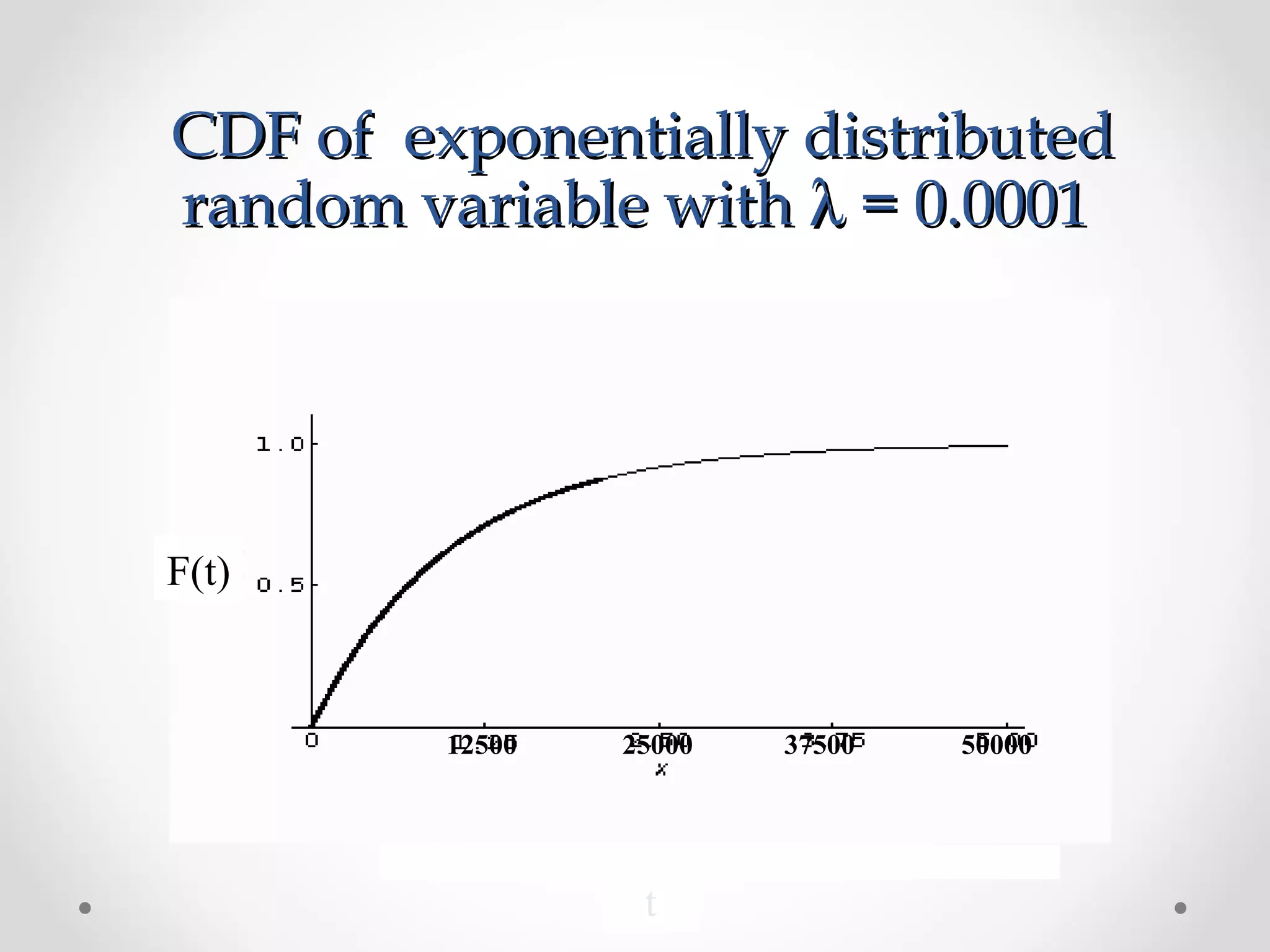
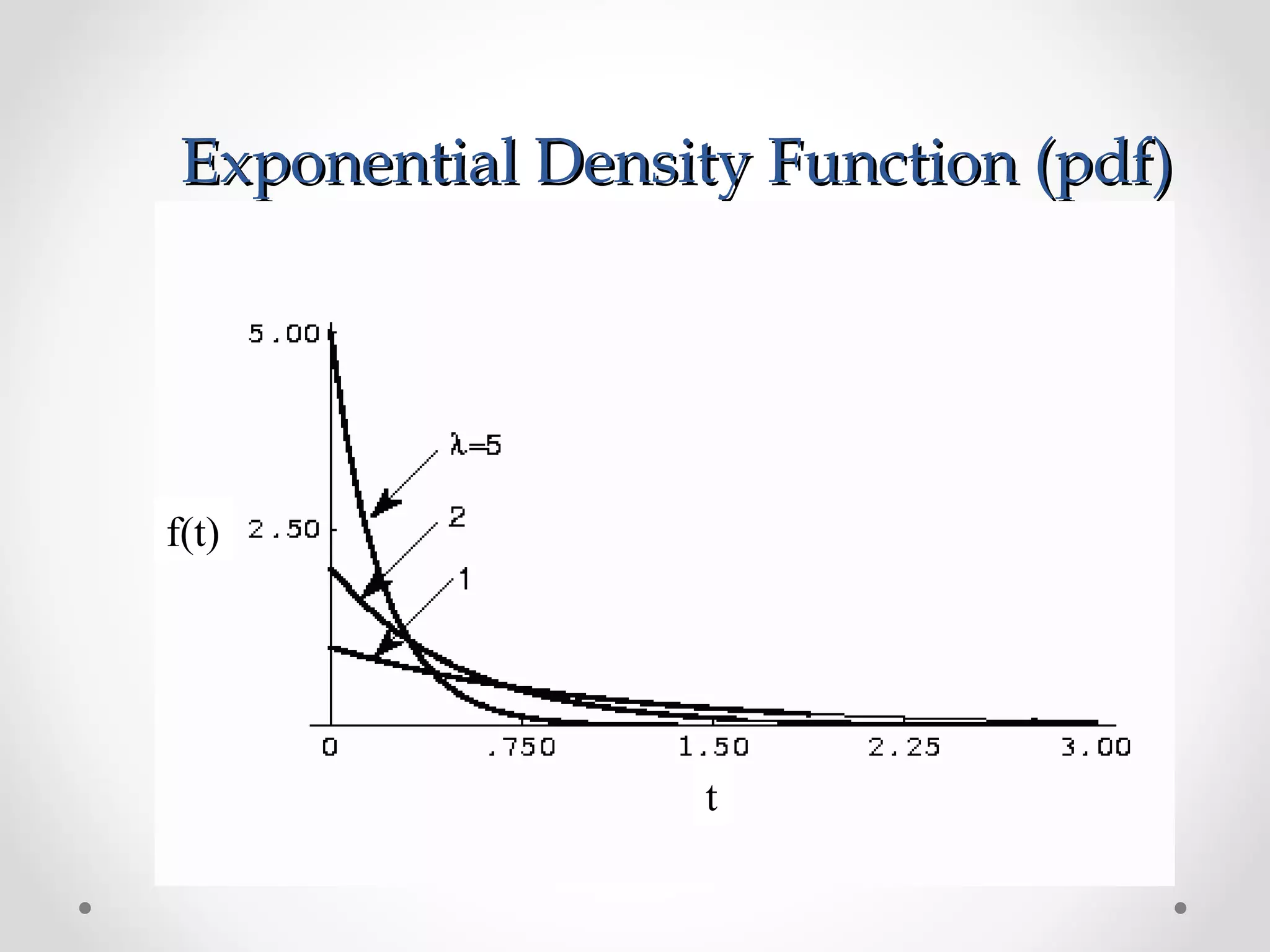
Discusses exponential distribution's application, properties, and mathematical definitions.
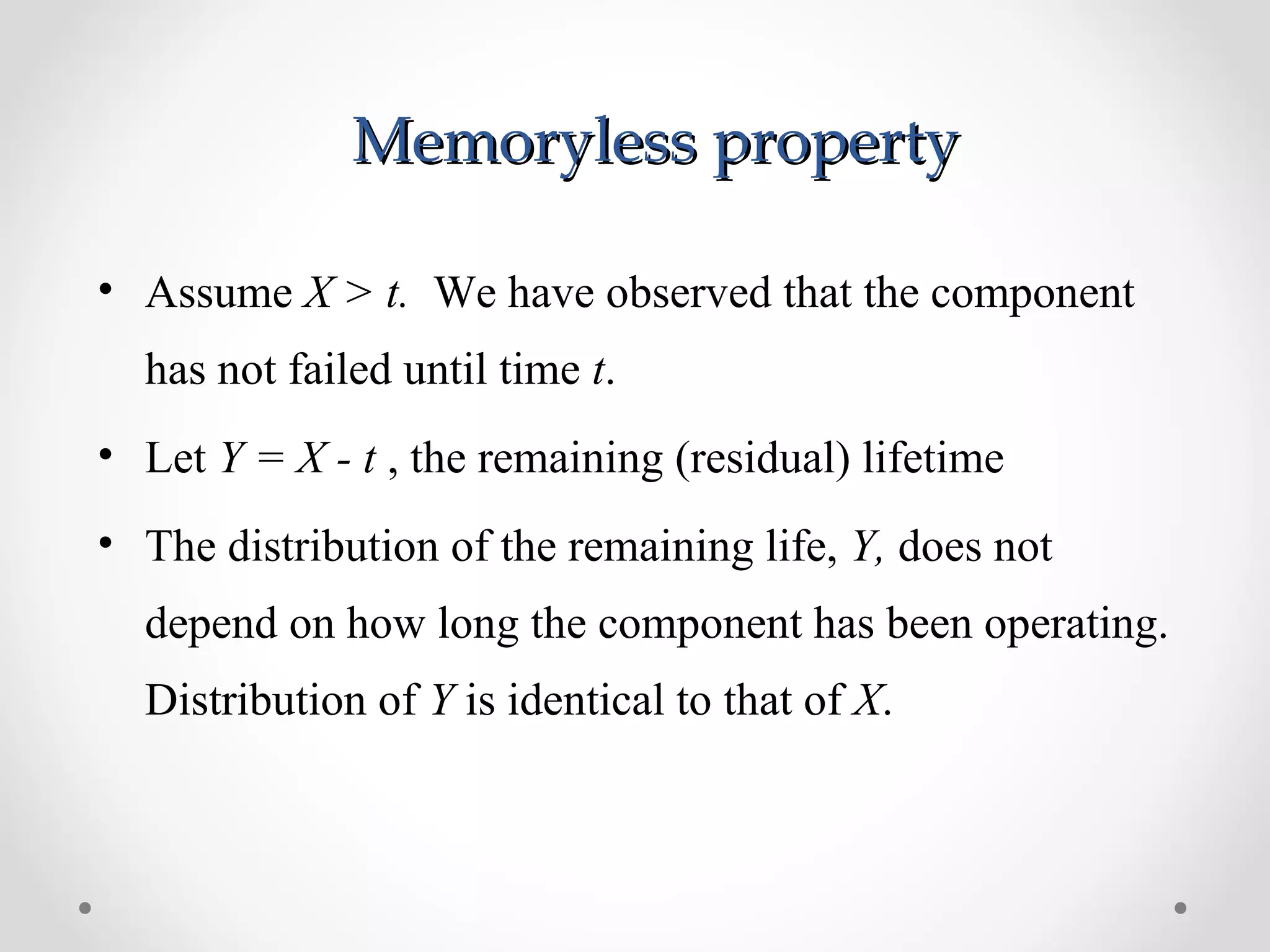
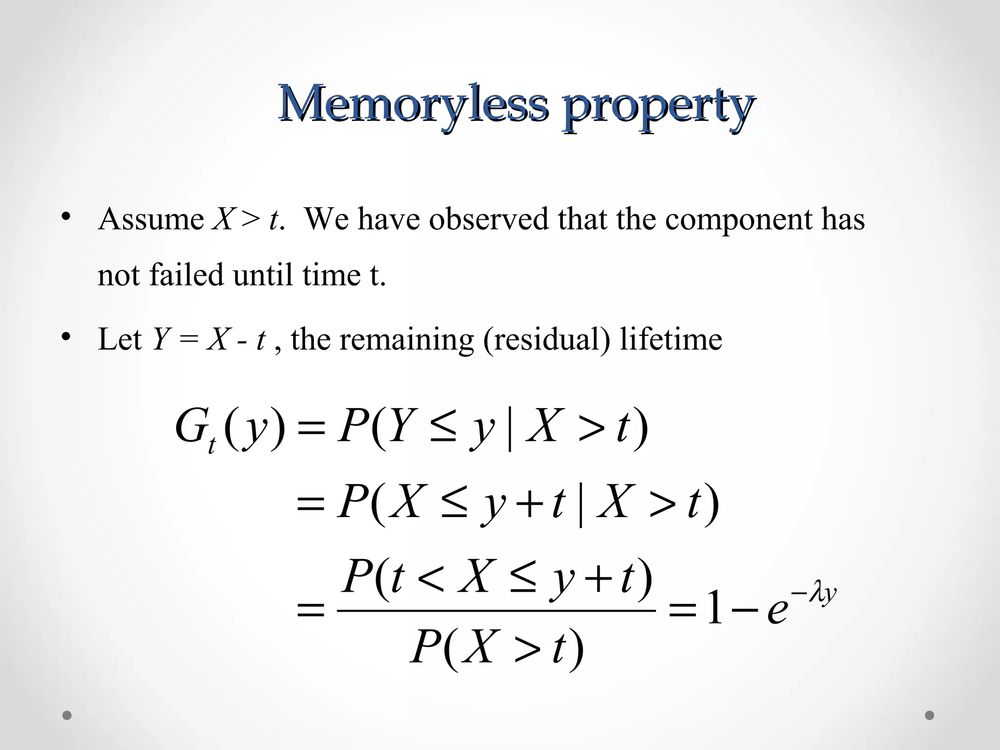
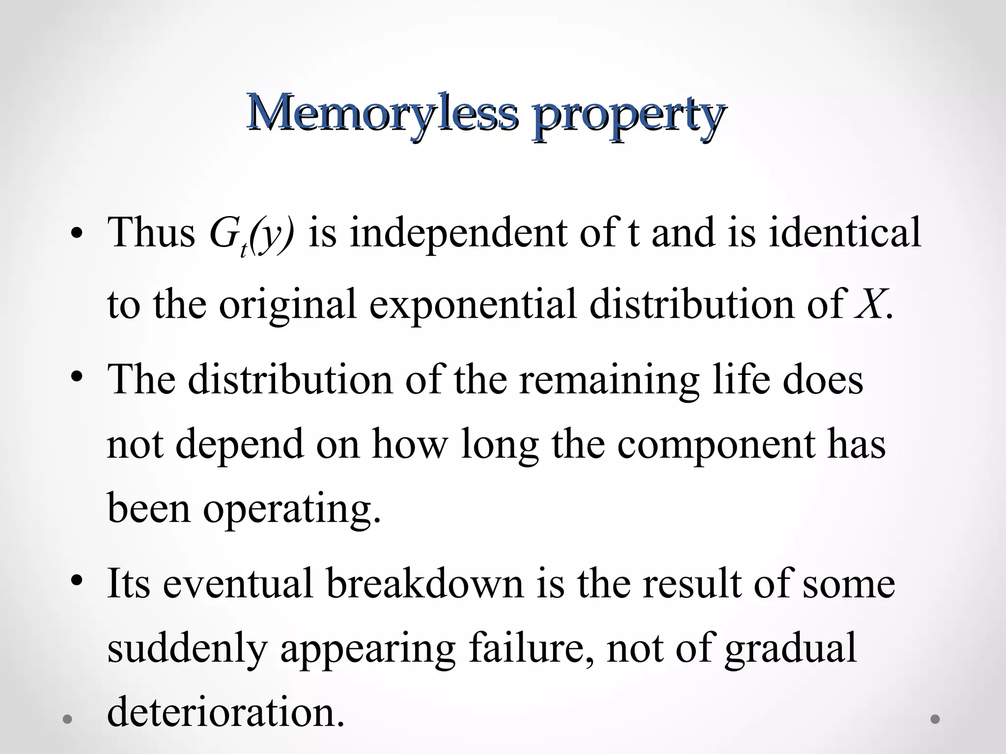
Explains the memoryless property of exponential distributions, related to residual lifetime.
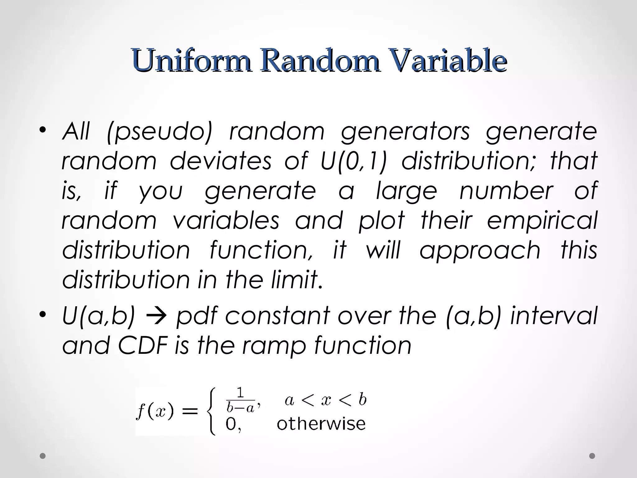
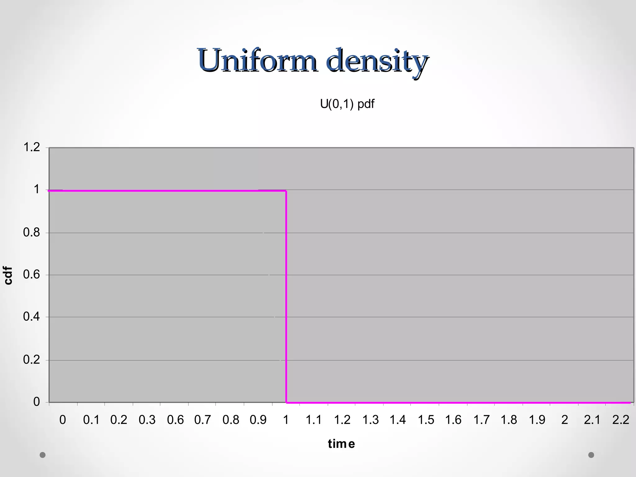
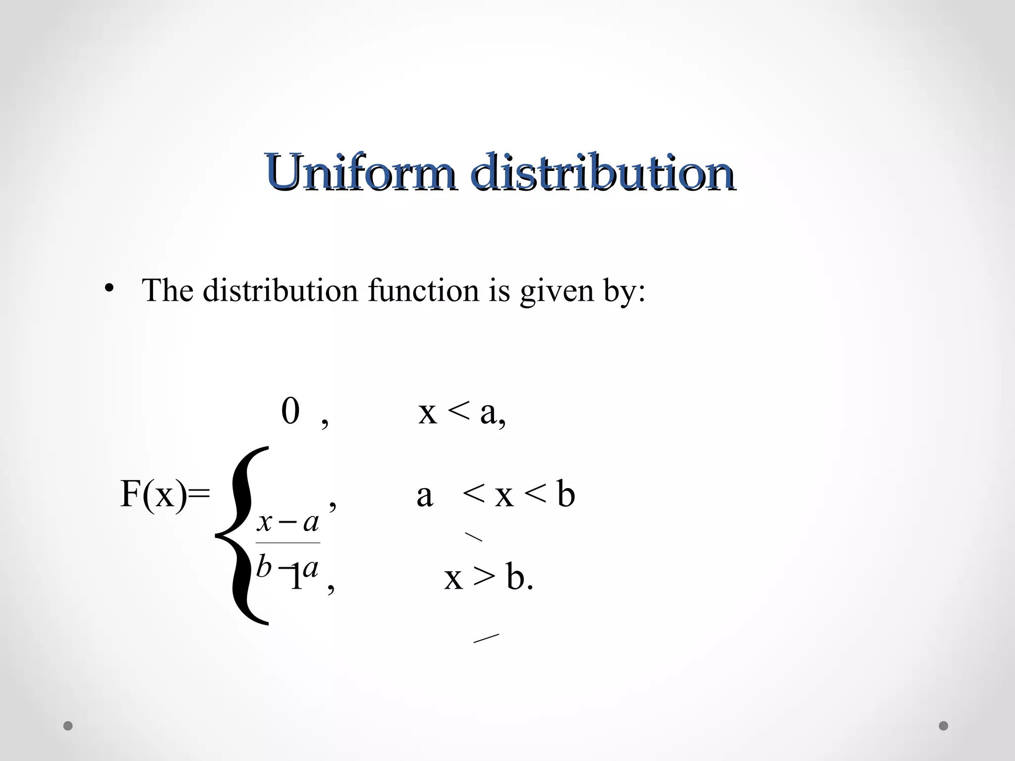
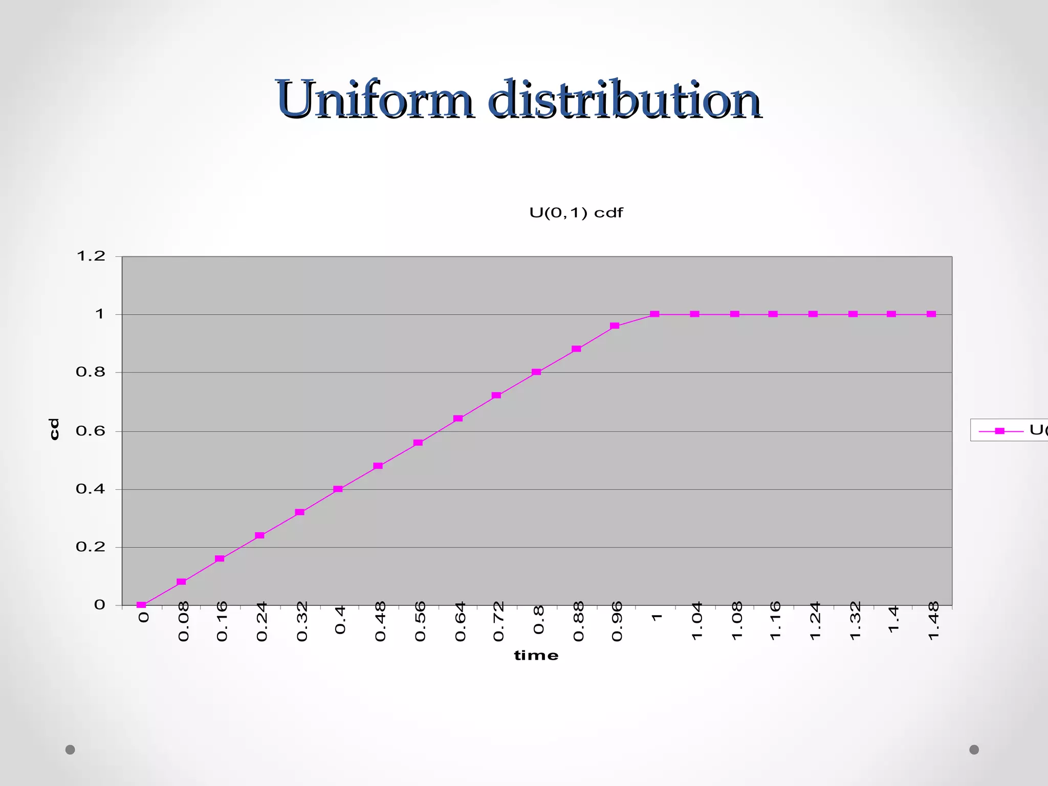
Describes uniform random variables, their random generation properties, pdf, and cdf.
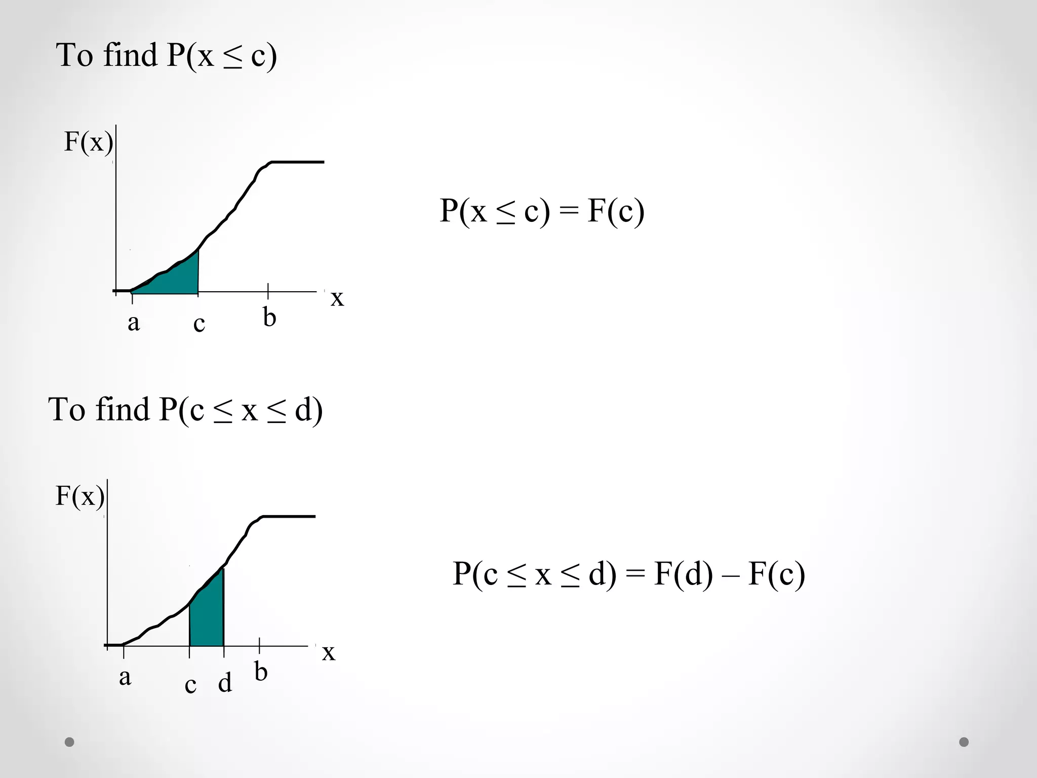
Demonstrates how to use cumulative distribution function (CDF) for probability calculations.


![ANPARA THERMAL POWER STATION[1] sangam.pdf](https://cdn.slidesharecdn.com/ss_thumbnails/anparathermalpowerstation1sangam-251121115219-9261cde4-thumbnail.jpg?width=640&height=640&fit=bounds)


