Downloaded 30 times
![Snehal Patel Soft Computing Research Paper En. No: 090330131025
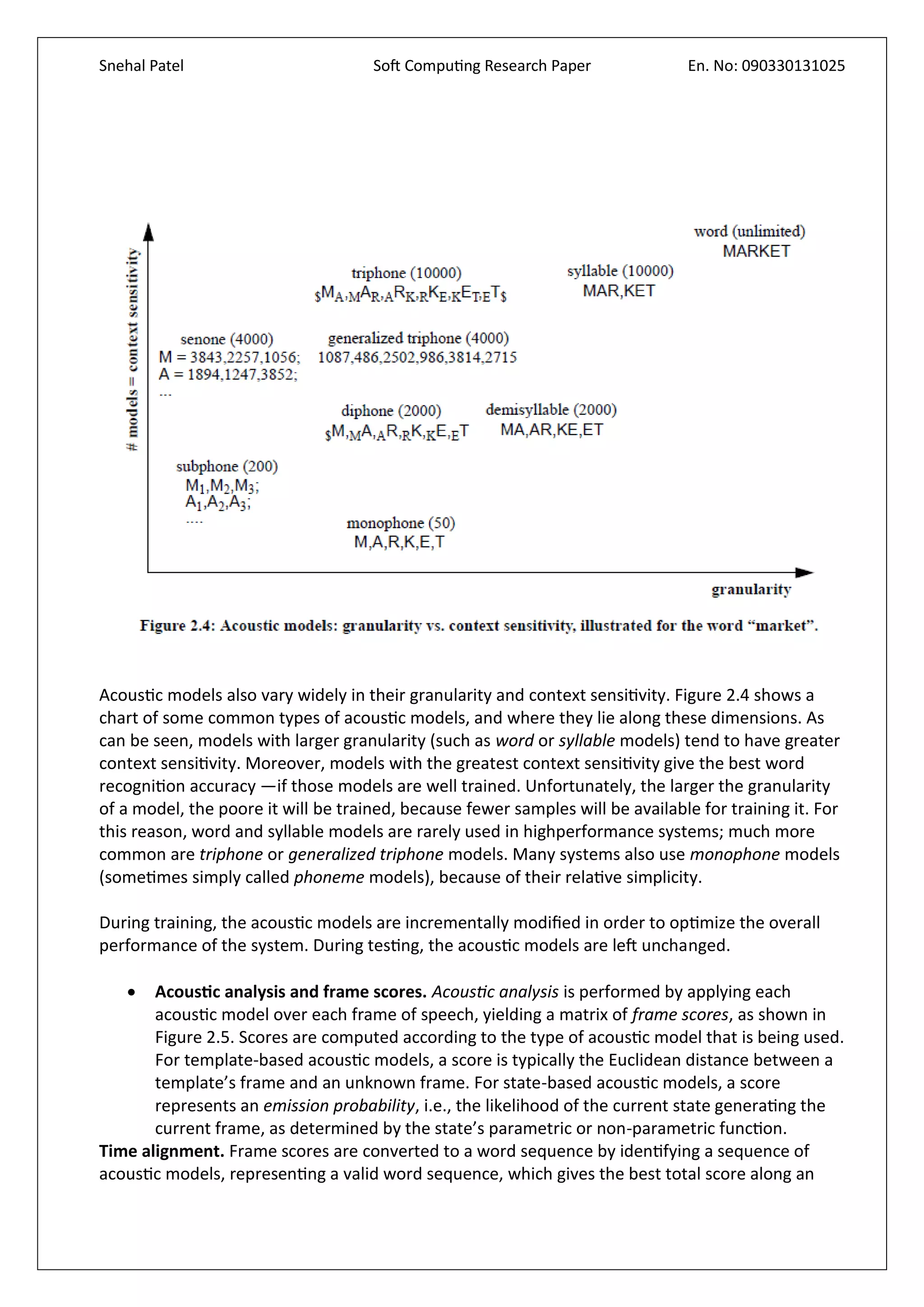
Pre-processing and Feature Extraction
Human speech can be represented as an analog wave that varies over time. The height of the
wave represents intensity (loudness), and the shape of the wave represents frequency (pitch). The
properties of the speech signal changes relatively slowly with time. This allows examination of a
Short-time window of speech to extract parameters presumed to remain fixed for the duration of
the window. The signal must be divided into successive windows or analysis frames so that the
parameters can be calculated often enough to follow the relevant changes. The result of signal
analysis is a sequence of speech frames. To extract the features from the speech signal, the signal
must be preprocessed and divided into successive windows or analysis frames.
Each sentence was taken through different stages of preprocessing which included Preemphasis,
Frame Processing and Windowing [5, 8]. The higher frequencies of the speech signal are
generally weak. As a result there may not be high frequency energy present to extract features at
the upper end of the frequency range. Pre-emphasis is used to boost the energy of the high
frequency signals. Frame blocking is a process adopted to split the speech signal into frames
The speech samples are segmented into 32 ms frames with each frame having 50% overlap
with the adjacent frames. The next step in preprocessing is to window each individual frame so as
to minimize the signal discontinuities at the beginning and end of the frame. To minimize the
signal discontinuities Hamming window is used which has the form.
The purpose of feature extraction is to represent the speech signal by a finite number of
measures of the signal. It gives the invariant representations in the signal. The features selected
are the Short Time Average Zero Crossing Rate [7], Pitch Period Computation, Mel Frequency
Cepstral Coefficients (MFCC), Formants and Modulation Index. The more features we use, the
better the representation.](https://image.slidesharecdn.com/speechrecognitionusingneuralfuzzylogic-161018201804/75/Speech-recognition-using-neural-fuzzy-logic-14-2048.jpg)


![Snehal Patel Soft Computing Research Paper En. No: 090330131025
Pre-processing and Feature Extraction
Human speech can be represented as an analog wave that varies over time. The height of the
wave represents intensity (loudness), and the shape of the wave represents frequency (pitch). The
properties of the speech signal changes relatively slowly with time. This allows examination of a
Short-time window of speech to extract parameters presumed to remain fixed for the duration of
the window. The signal must be divided into successive windows or analysis frames so that the
parameters can be calculated often enough to follow the relevant changes. The result of signal
analysis is a sequence of speech frames. To extract the features from the speech signal, the signal
must be preprocessed and divided into successive windows or analysis frames.
Each sentence was taken through different stages of preprocessing which included Preemphasis,
Frame Processing and Windowing [5, 8]. The higher frequencies of the speech signal are
generally weak. As a result there may not be high frequency energy present to extract features at
the upper end of the frequency range. Pre-emphasis is used to boost the energy of the high
frequency signals. Frame blocking is a process adopted to split the speech signal into frames
The speech samples are segmented into 32 ms frames with each frame having 50% overlap
with the adjacent frames. The next step in preprocessing is to window each individual frame so as
to minimize the signal discontinuities at the beginning and end of the frame. To minimize the
signal discontinuities Hamming window is used which has the form.
The purpose of feature extraction is to represent the speech signal by a finite number of
measures of the signal. It gives the invariant representations in the signal. The features selected
are the Short Time Average Zero Crossing Rate [7], Pitch Period Computation, Mel Frequency
Cepstral Coefficients (MFCC), Formants and Modulation Index. The more features we use, the
better the representation.](https://crownmelresort.com/image.slidesharecdn.com/speechrecognitionusingneuralfuzzylogic-161018201804/75/Speech-recognition-using-neural-fuzzy-logic-14-2048.jpg)


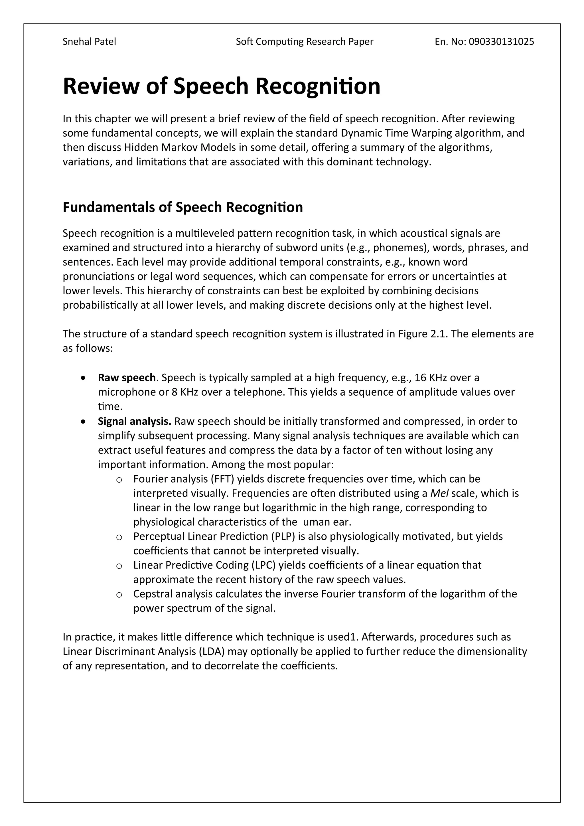
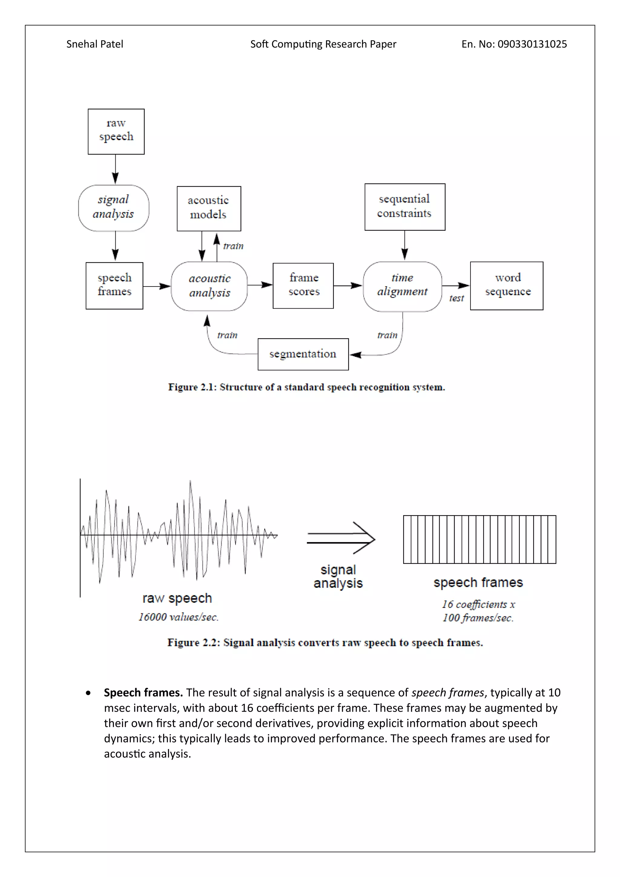
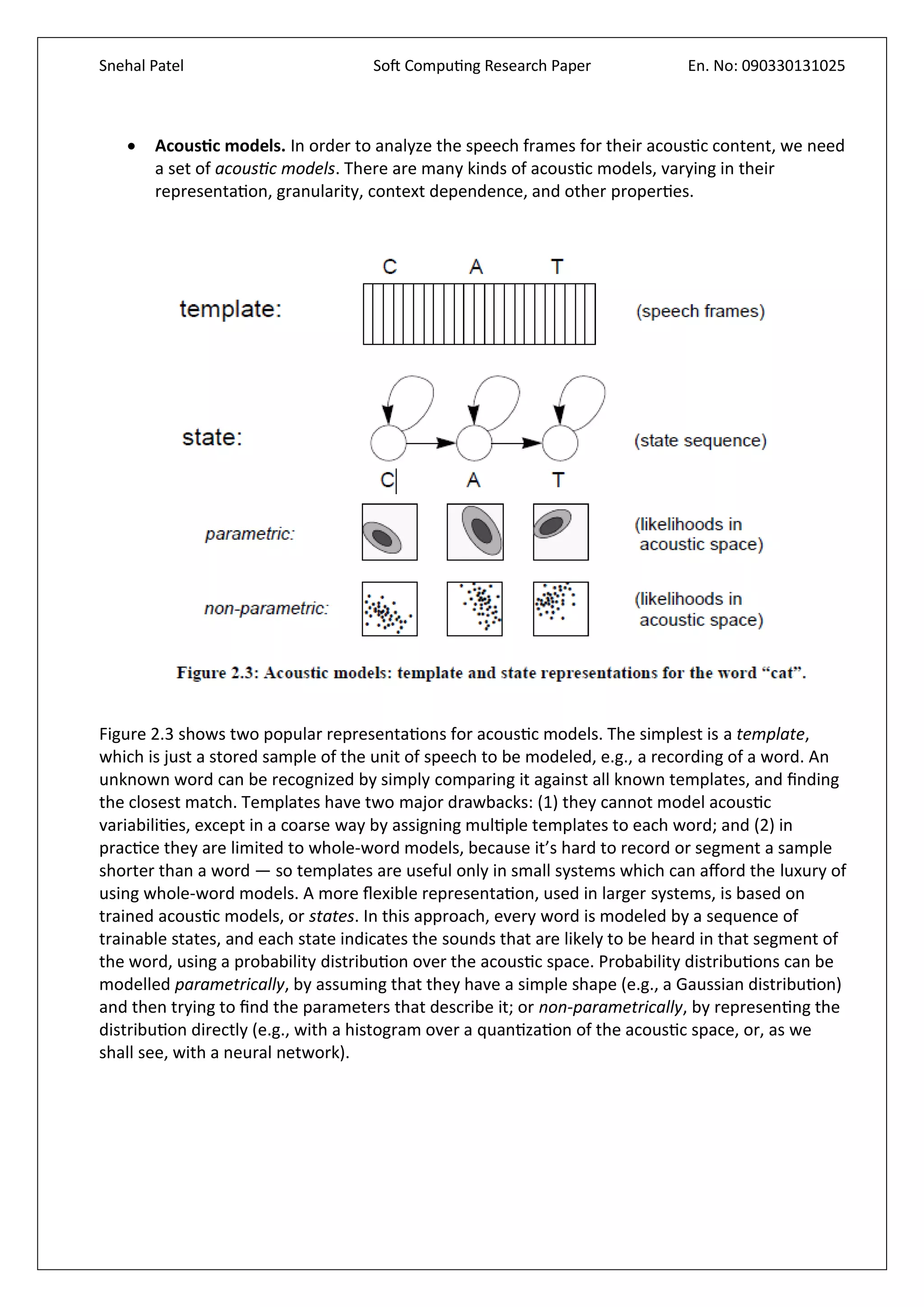
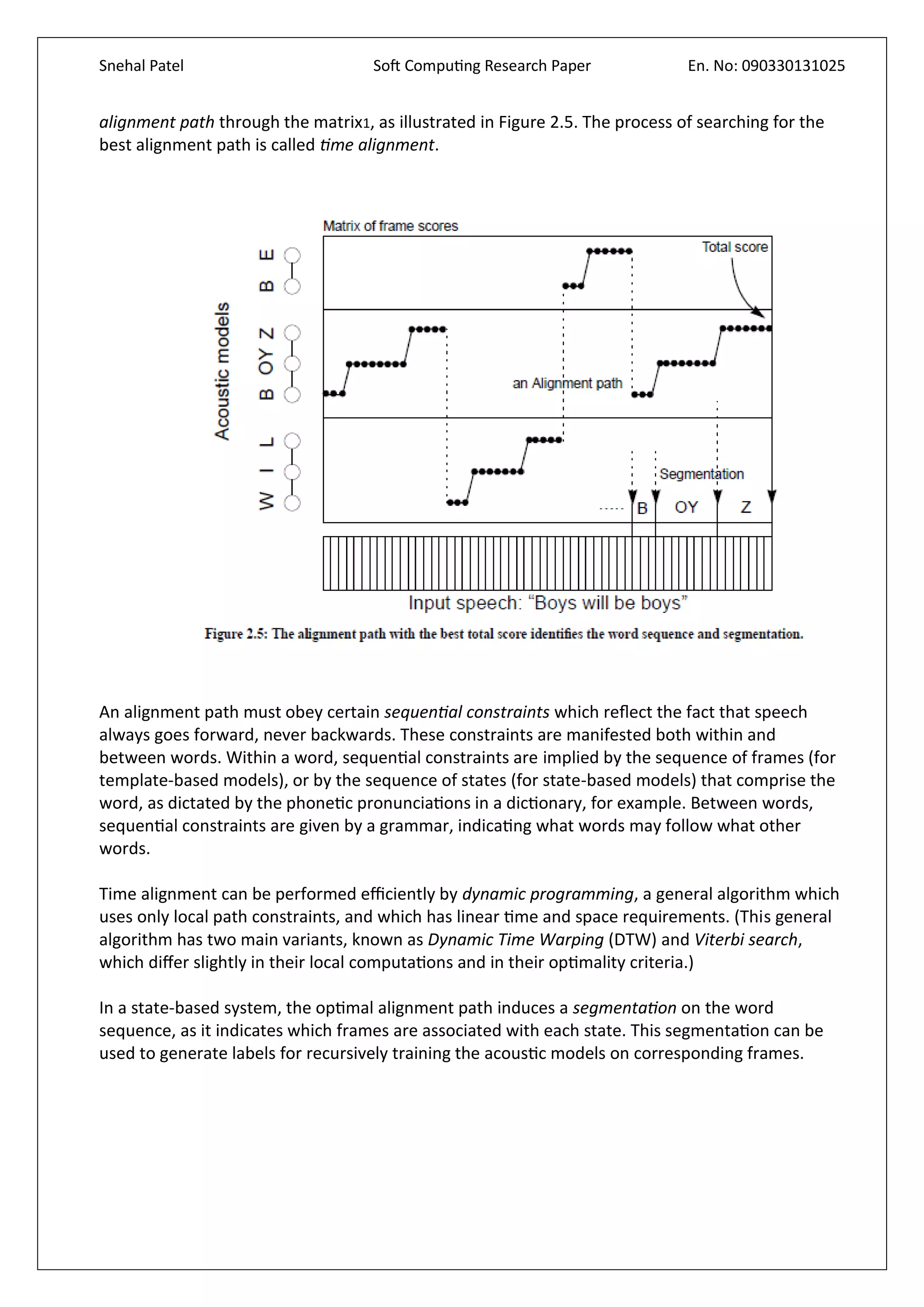
This research paper explores the use of artificial neural networks (ANN) for improving continuous speech recognition systems, traditionally dominated by hidden Markov models (HMM). The thesis presents a hybrid NN-HMM approach, demonstrating superior word accuracy and better modeling capabilities than HMM alone, while also addressing challenges such as speaker variability and environmental noise. Key findings highlight the advantages of neural networks in acoustic modeling and the comparative performance of different recognition models, emphasizing the potential for ANN to enhance speech recognition technology.