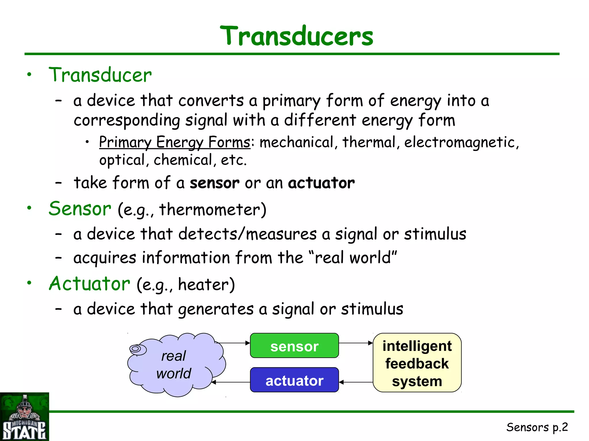
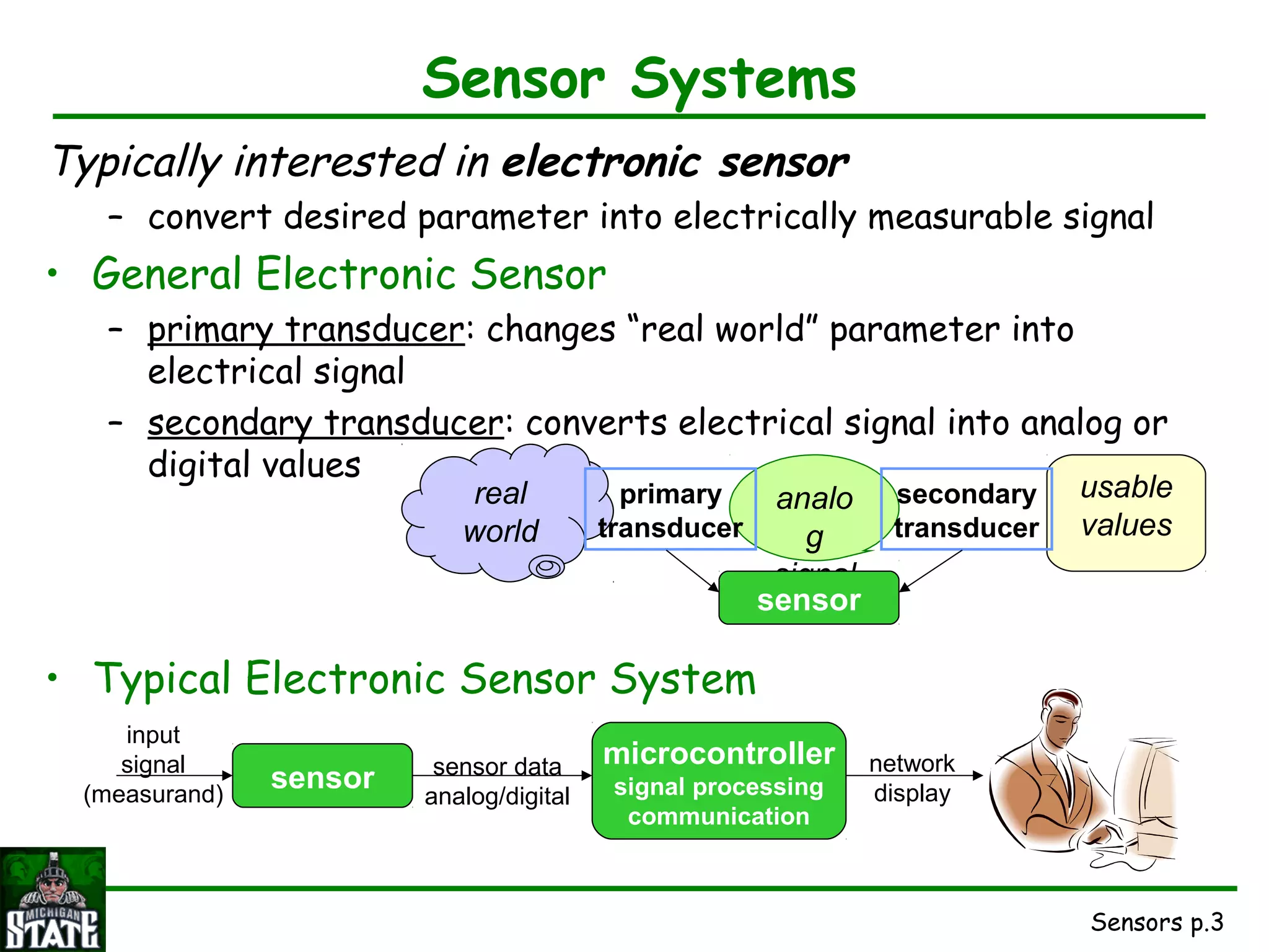
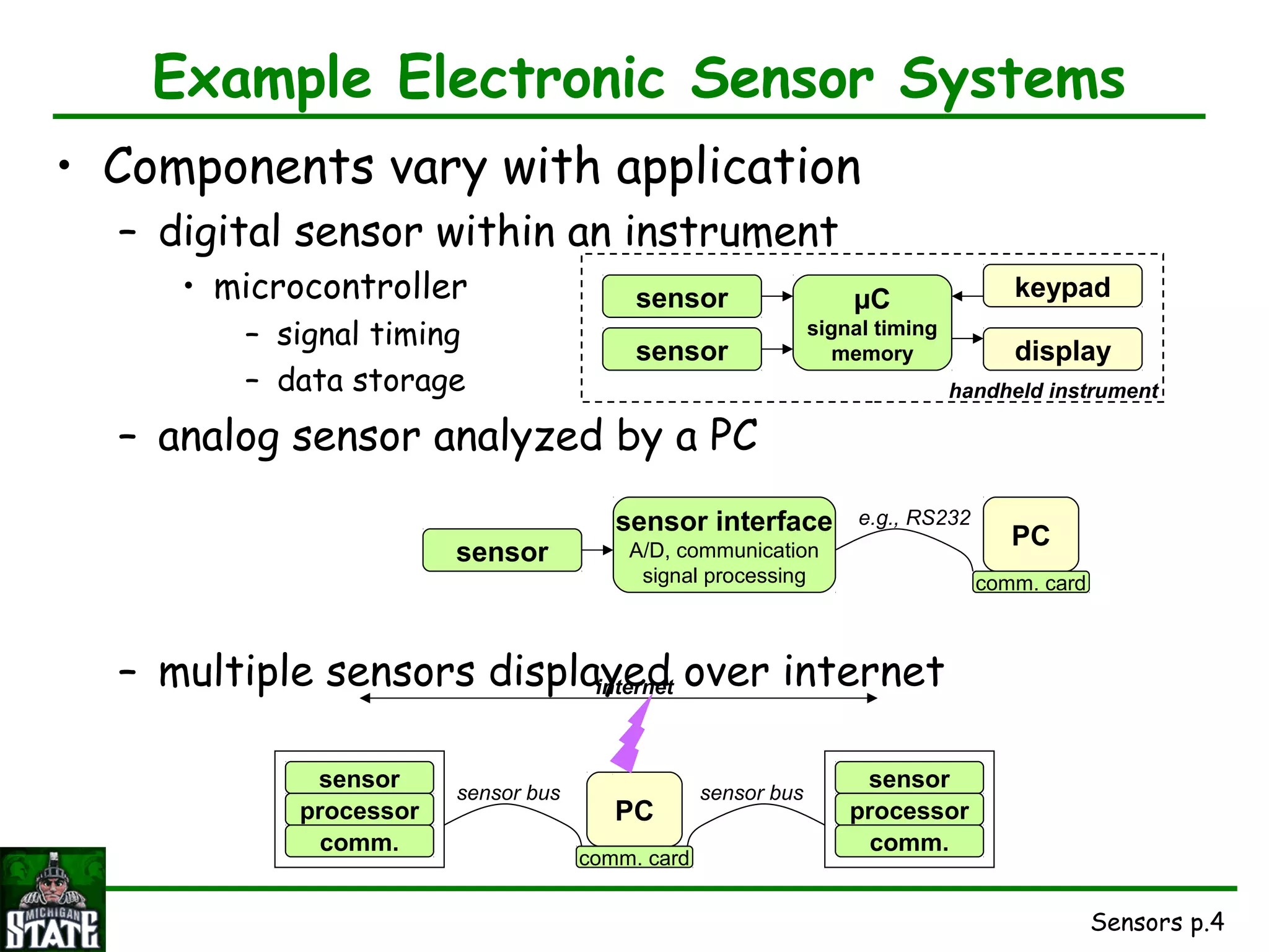
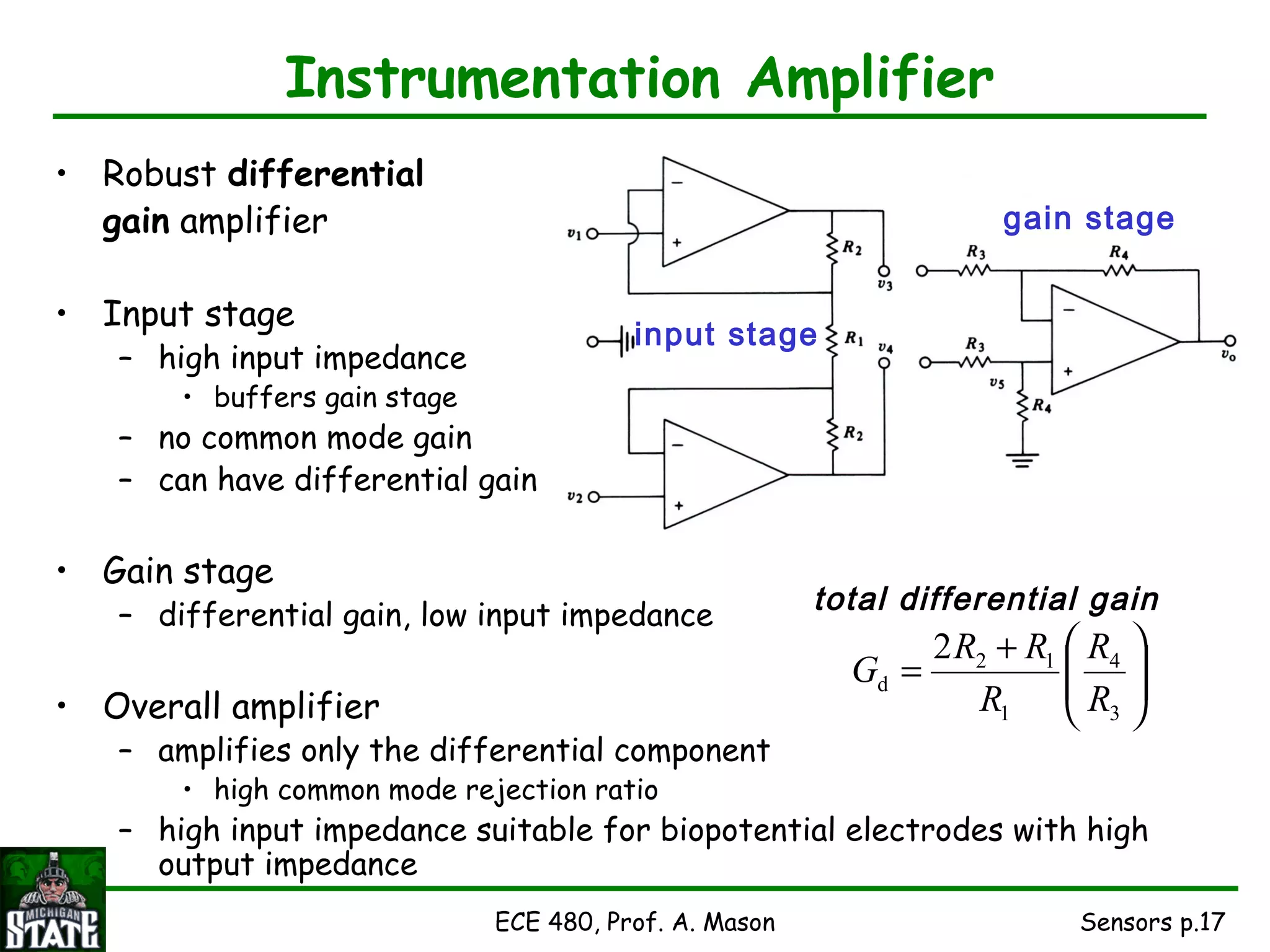
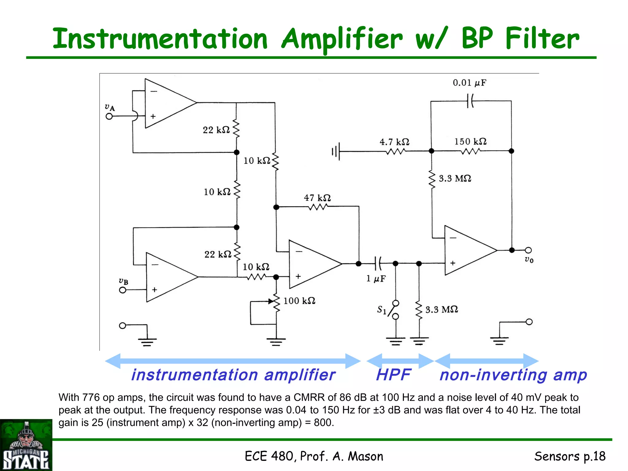
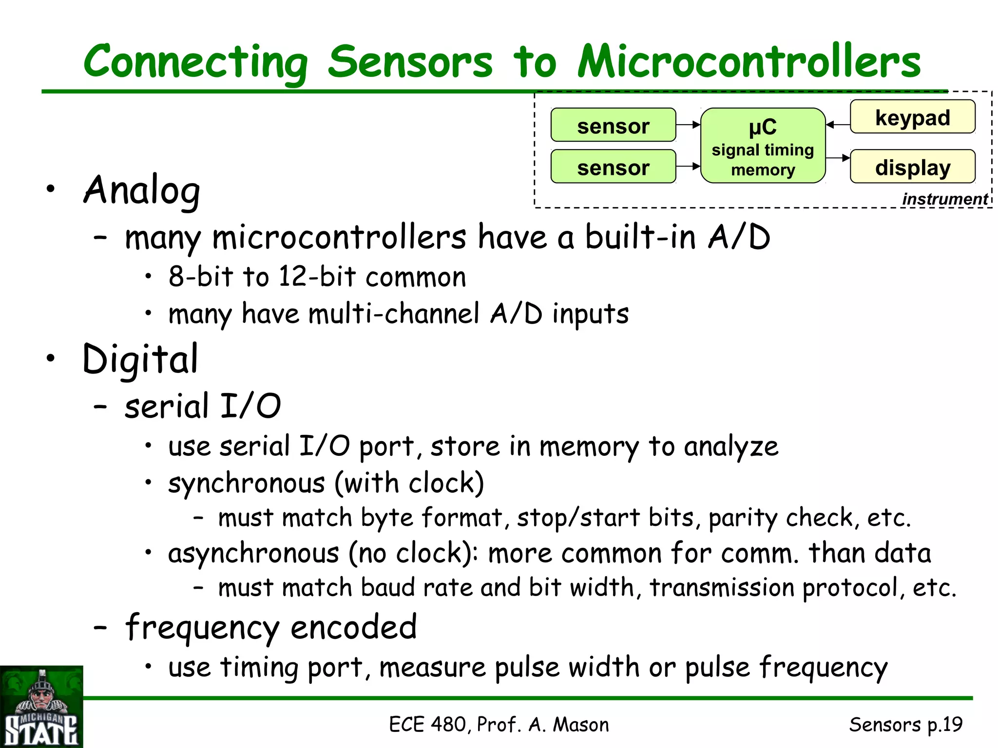
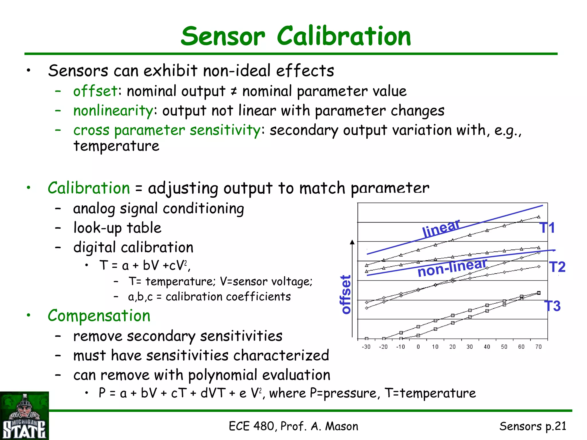
Sensors p.1
SENSORS
Interfacing to the Real World:
Review of Electrical Sensors and Actuators
Sensors p.2
Transducers
• Transducer
– a device that converts a primary form of energy into a
corresponding signal with a different energy form
• Primary Energy Forms: mechanical, thermal, electromagnetic,
optical, chemical, etc.
– take form of a sensor or an actuator
• Sensor (e.g., thermometer)
– a device that detects/measures a signal or stimulus
– acquires information from the “real world”
• Actuator (e.g., heater)
– a device that generates a signal or stimulus
real
world
sensor
actuator
intelligent
feedback
system
Sensors p.3
usable
values
Sensor Systems
Typically interested in electronic sensor
– convert desired parameter into electrically measurable signal
• General Electronic Sensor
– primary transducer: changes “real world” parameter into
electrical signal
– secondary transducer: converts electrical signal into analog or
digital values
• Typical Electronic Sensor System
real
world
analo
g
signal
primary
transducer
secondary
transducer
sensor
sensor
input
signal
(measurand)
microcontroller
signal processing
communication
sensor data
analog/digital
network
display
Sensors p.4
Example Electronic Sensor Systems
• Components vary with application
– digital sensor within an instrument
• microcontroller
– signal timing
– data storage
– analog sensor analyzed by a PC
– multiple sensors displayed over internet
µC
signal timing
memory
keypadsensor
sensor display
handheld instrument
PC
comm. card
sensor interface
A/D, communication
signal processing
sensor
e.g., RS232
PC
comm. card
internet
sensor
processor
comm.
sensor
processor
comm.
sensor bus sensor bus
Sensors p.5
Primary Transducers
• Conventional Transducers
large, but generally reliable, based on older technology
– thermocouple: temperature difference
– compass (magnetic): direction
• Microelectronic Sensors
millimeter sized, highly sensitive, less robust
– photodiode/phototransistor: photon energy (light)
• infrared detectors, proximity/intrusion alarms
– piezoresisitve pressure sensor: air/fluid pressure
– microaccelerometers: vibration, ∆-velocity (car crash)
– chemical senors: O2, CO2, Cl, Nitrates (explosives)
– DNA arrays: match DNA sequences
Sensors p.6ECE 480, Prof. A. Mason
Example Primary Transducers
• Light Sensor
– photoconductor
• light  ∆R
– photodiode
• light  ∆I
– membrane pressure sensor
• resistive (pressure  ∆ R)
• capacitive (pressure  ∆C)
Sensors p.7ECE 480, Prof. A. Mason
Displacement Measurements
• Measurements of size, shape, and position utilize
displacement sensors
• Examples
– diameter of part under stress (direct)
– movement of a microphone diaphragm to quantify liquid
movement through the heart (indirect)
• Primary Transducer Types
– Resistive Sensors (Potentiometers & Strain Gages)
– Inductive Sensors
– Capacitive Sensors
– Piezoelectric Sensors
• Secondary Transducers
– Wheatstone Bridge
– Amplifiers
Sensors p.8ECE 480, Prof. A. Mason
Strain Gage: Gage Factor
• Remember: for a strained thin wire
– ∆R/R = ∆L/L – ∆A/A + ∆ρ/ρ
• A = π (D/2)2
, for circular wire
• Poisson’s ratio, µ: relates change in diameter D to
change in length L
– ∆D/D = - µ ∆L/L
• Thus
– ∆R/R = (1+2µ) ∆L/L + ∆ρ/ρ
• Gage Factor, G, used to compare strain-gate materials
– G = ∆R/R = (1+2µ) + ∆ρ/ρ
∆L/L ∆L/L
LD
dimensional effect piezoresistive effect
Sensors p.9
Temperature Sensor Options
• Resistance Temperature Detectors (RTDs)
– Platinum, Nickel, Copper metals are typically used
– positive temperature coefficients
• Thermistors (“thermally sensitive resistor”)
– formed from semiconductor materials, not metals
• often composite of a ceramic and a metallic oxide (Mn, Co, Cu or Fe)
– typically have negative temperature coefficients
• Thermocouples
– based on the Seebeck effect: dissimilar metals at diff. temps.  signal
Sensors p.10
Fiber-optic Temperature Sensor
• Sensor operation
– small prism-shaped sample of single-crystal undoped GaAs
attached to ends of two optical fibers
– light energy absorbed by the GaAs crystal depends on
temperature
– percentage of received vs. transmitted energy is a function of
temperature
• Can be made small enough for biological implantation
GaAs semiconductor temperature probe
Sensors p.11
Example MEMS Transducers
• MEMS = micro-electro-mechanical system
– miniature transducers created using IC fabrication processes
• Microaccelerometer
– cantilever beam
– suspended mass
• Rotation
– gyroscope
• Pressure
Electrodes
Ring
structure
Diaphragm (Upper electrode)
Lower electrode 5-10mm
Sensors p.12ECE 480, Prof. A. Mason
Passive Sensor Readout Circuit
• Photodiode Circuits
• Thermistor Half-Bridge
– voltage divider
– one element varies
• Wheatstone Bridge
– R3 = resistive sensor
– R4 is matched to nominal value of R3
– If R1 = R2, Vout-nominal = 0
– Vout varies as R3 changes
VCC
R1+R4
Sensors p.13ECE 480, Prof. A. Mason
Operational Amplifiers
• Properties
– open-loop gain: ideally infinite: practical values 20k-200k
•high open-loop gain  virtual short between + and - inputs
– input impedance: ideally infinite: CMOS opamps are close to ideal
– output impedance: ideally zero: practical values 20-100Ω
– zero output offset: ideally zero: practical value <1mV
– gain-bandwidth product (GB): practical values ~MHz
•frequency where open-loop gain drops to 1 V/V
• Commercial opamps provide many different properties
– low noise
– low input current
– low power
– high bandwidth
– low/high supply voltage
– special purpose: comparator, instrumentation amplifier
Sensors p.14
Basic Opamp Configuration
• Voltage Comparator
– digitize input
• Voltage Follower
– buffer
• Non-Inverting Amp • Inverting Amp
Sensors p.15ECE 480, Prof. A. Mason
More Opamp Configurations
• Summing Amp
• Differential Amp
• Integrating Amp
• Differentiating Amp
Sensors p.16ECE 480, Prof. A. Mason
Converting Configuration
• Current-to-Voltage
• Voltage-to-Current
Sensors p.17ECE 480, Prof. A. Mason
Instrumentation Amplifier
• Robust differential
gain amplifier
• Input stage
– high input impedance
• buffers gain stage
– no common mode gain
– can have differential gain
• Gain stage
– differential gain, low input impedance
• Overall amplifier
– amplifies only the differential component
• high common mode rejection ratio
– high input impedance suitable for biopotential electrodes with high
output impedance
input stage
gain stage





+
=
3
4
1
12
d
2
R
R
R
RR
G
total differential gain
Sensors p.18ECE 480, Prof. A. Mason
Instrumentation Amplifier w/ BP Filter
instrumentation amplifier
With 776 op amps, the circuit was found to have a CMRR of 86 dB at 100 Hz and a noise level of 40 mV peak to
peak at the output. The frequency response was 0.04 to 150 Hz for ±3 dB and was flat over 4 to 40 Hz. The total
gain is 25 (instrument amp) x 32 (non-inverting amp) = 800.
HPF non-inverting amp
Sensors p.19ECE 480, Prof. A. Mason
Connecting Sensors to Microcontrollers
• Analog
– many microcontrollers have a built-in A/D
• 8-bit to 12-bit common
• many have multi-channel A/D inputs
• Digital
– serial I/O
• use serial I/O port, store in memory to analyze
• synchronous (with clock)
– must match byte format, stop/start bits, parity check, etc.
• asynchronous (no clock): more common for comm. than data
– must match baud rate and bit width, transmission protocol, etc.
– frequency encoded
• use timing port, measure pulse width or pulse frequency
µC
signal timing
memory
keypadsensor
sensor display
instrument
Sensors p.20ECE 480, Prof. A. Mason
Connecting Smart Sensors to PC/Network
• “Smart sensor” = sensor with built-in signal processing & communication
– e.g., combining a “dumb sensor” and a microcontroller
• Data Acquisition Cards (DAQ)
– PC card with analog and digital I/O
– interface through LabVIEW or user-generated code
• Communication Links Common for Sensors
– asynchronous serial comm.
• universal asynchronous receive and transmit (UART)
– 1 receive line + 1 transmit line. nodes must match baud rate & protocol
• RS232 Serial Port on PCs uses UART format (but at +/- 12V)
– can buy a chip to convert from UART to RS232
– synchronous serial comm.
• serial peripheral interface (SPI)
– 1 clock + 1 bidirectional data + 1 chip select/enable
– I2
C = Inter Integrated Circuit bus
• designed by Philips for comm. inside TVs, used in several commercial sensor systems
– IEEE P1451: Sensor Comm. Standard
• several different sensor comm. protocols for different applications
Sensors p.21ECE 480, Prof. A. Mason
Sensor Calibration
• Sensors can exhibit non-ideal effects
– offset: nominal output ≠ nominal parameter value
– nonlinearity: output not linear with parameter changes
– cross parameter sensitivity: secondary output variation with, e.g.,
temperature
• Calibration = adjusting output to match parameter
– analog signal conditioning
– look-up table
– digital calibration
• T = a + bV +cV2
,
– T= temperature; V=sensor voltage;
– a,b,c = calibration coefficients
• Compensation
– remove secondary sensitivities
– must have sensitivities characterized
– can remove with polynomial evaluation
• P = a + bV + cT + dVT + e V2
, where P=pressure, T=temperature
T1
T2
T3
offset
linear
non-linear

Sensor Lecture Interfacing

  • 1.
    Sensors p.1 SENSORS Interfacing tothe Real World: Review of Electrical Sensors and Actuators
  • 2.
    Sensors p.2 Transducers • Transducer –a device that converts a primary form of energy into a corresponding signal with a different energy form • Primary Energy Forms: mechanical, thermal, electromagnetic, optical, chemical, etc. – take form of a sensor or an actuator • Sensor (e.g., thermometer) – a device that detects/measures a signal or stimulus – acquires information from the “real world” • Actuator (e.g., heater) – a device that generates a signal or stimulus real world sensor actuator intelligent feedback system
  • 3.
    Sensors p.3 usable values Sensor Systems Typicallyinterested in electronic sensor – convert desired parameter into electrically measurable signal • General Electronic Sensor – primary transducer: changes “real world” parameter into electrical signal – secondary transducer: converts electrical signal into analog or digital values • Typical Electronic Sensor System real world analo g signal primary transducer secondary transducer sensor sensor input signal (measurand) microcontroller signal processing communication sensor data analog/digital network display
  • 4.
    Sensors p.4 Example ElectronicSensor Systems • Components vary with application – digital sensor within an instrument • microcontroller – signal timing – data storage – analog sensor analyzed by a PC – multiple sensors displayed over internet µC signal timing memory keypadsensor sensor display handheld instrument PC comm. card sensor interface A/D, communication signal processing sensor e.g., RS232 PC comm. card internet sensor processor comm. sensor processor comm. sensor bus sensor bus
  • 5.
    Sensors p.5 Primary Transducers •Conventional Transducers large, but generally reliable, based on older technology – thermocouple: temperature difference – compass (magnetic): direction • Microelectronic Sensors millimeter sized, highly sensitive, less robust – photodiode/phototransistor: photon energy (light) • infrared detectors, proximity/intrusion alarms – piezoresisitve pressure sensor: air/fluid pressure – microaccelerometers: vibration, ∆-velocity (car crash) – chemical senors: O2, CO2, Cl, Nitrates (explosives) – DNA arrays: match DNA sequences
  • 6.
    Sensors p.6ECE 480,Prof. A. Mason Example Primary Transducers • Light Sensor – photoconductor • light  ∆R – photodiode • light  ∆I – membrane pressure sensor • resistive (pressure  ∆ R) • capacitive (pressure  ∆C)
  • 7.
    Sensors p.7ECE 480,Prof. A. Mason Displacement Measurements • Measurements of size, shape, and position utilize displacement sensors • Examples – diameter of part under stress (direct) – movement of a microphone diaphragm to quantify liquid movement through the heart (indirect) • Primary Transducer Types – Resistive Sensors (Potentiometers & Strain Gages) – Inductive Sensors – Capacitive Sensors – Piezoelectric Sensors • Secondary Transducers – Wheatstone Bridge – Amplifiers
  • 8.
    Sensors p.8ECE 480,Prof. A. Mason Strain Gage: Gage Factor • Remember: for a strained thin wire – ∆R/R = ∆L/L – ∆A/A + ∆ρ/ρ • A = π (D/2)2 , for circular wire • Poisson’s ratio, µ: relates change in diameter D to change in length L – ∆D/D = - µ ∆L/L • Thus – ∆R/R = (1+2µ) ∆L/L + ∆ρ/ρ • Gage Factor, G, used to compare strain-gate materials – G = ∆R/R = (1+2µ) + ∆ρ/ρ ∆L/L ∆L/L LD dimensional effect piezoresistive effect
  • 9.
    Sensors p.9 Temperature SensorOptions • Resistance Temperature Detectors (RTDs) – Platinum, Nickel, Copper metals are typically used – positive temperature coefficients • Thermistors (“thermally sensitive resistor”) – formed from semiconductor materials, not metals • often composite of a ceramic and a metallic oxide (Mn, Co, Cu or Fe) – typically have negative temperature coefficients • Thermocouples – based on the Seebeck effect: dissimilar metals at diff. temps.  signal
  • 10.
    Sensors p.10 Fiber-optic TemperatureSensor • Sensor operation – small prism-shaped sample of single-crystal undoped GaAs attached to ends of two optical fibers – light energy absorbed by the GaAs crystal depends on temperature – percentage of received vs. transmitted energy is a function of temperature • Can be made small enough for biological implantation GaAs semiconductor temperature probe
  • 11.
    Sensors p.11 Example MEMSTransducers • MEMS = micro-electro-mechanical system – miniature transducers created using IC fabrication processes • Microaccelerometer – cantilever beam – suspended mass • Rotation – gyroscope • Pressure Electrodes Ring structure Diaphragm (Upper electrode) Lower electrode 5-10mm
  • 12.
    Sensors p.12ECE 480,Prof. A. Mason Passive Sensor Readout Circuit • Photodiode Circuits • Thermistor Half-Bridge – voltage divider – one element varies • Wheatstone Bridge – R3 = resistive sensor – R4 is matched to nominal value of R3 – If R1 = R2, Vout-nominal = 0 – Vout varies as R3 changes VCC R1+R4
  • 13.
    Sensors p.13ECE 480,Prof. A. Mason Operational Amplifiers • Properties – open-loop gain: ideally infinite: practical values 20k-200k •high open-loop gain  virtual short between + and - inputs – input impedance: ideally infinite: CMOS opamps are close to ideal – output impedance: ideally zero: practical values 20-100Ω – zero output offset: ideally zero: practical value <1mV – gain-bandwidth product (GB): practical values ~MHz •frequency where open-loop gain drops to 1 V/V • Commercial opamps provide many different properties – low noise – low input current – low power – high bandwidth – low/high supply voltage – special purpose: comparator, instrumentation amplifier
  • 14.
    Sensors p.14 Basic OpampConfiguration • Voltage Comparator – digitize input • Voltage Follower – buffer • Non-Inverting Amp • Inverting Amp
  • 15.
    Sensors p.15ECE 480,Prof. A. Mason More Opamp Configurations • Summing Amp • Differential Amp • Integrating Amp • Differentiating Amp
  • 16.
    Sensors p.16ECE 480,Prof. A. Mason Converting Configuration • Current-to-Voltage • Voltage-to-Current
  • 17.
    Sensors p.17ECE 480,Prof. A. Mason Instrumentation Amplifier • Robust differential gain amplifier • Input stage – high input impedance • buffers gain stage – no common mode gain – can have differential gain • Gain stage – differential gain, low input impedance • Overall amplifier – amplifies only the differential component • high common mode rejection ratio – high input impedance suitable for biopotential electrodes with high output impedance input stage gain stage      + = 3 4 1 12 d 2 R R R RR G total differential gain
  • 18.
    Sensors p.18ECE 480,Prof. A. Mason Instrumentation Amplifier w/ BP Filter instrumentation amplifier With 776 op amps, the circuit was found to have a CMRR of 86 dB at 100 Hz and a noise level of 40 mV peak to peak at the output. The frequency response was 0.04 to 150 Hz for ±3 dB and was flat over 4 to 40 Hz. The total gain is 25 (instrument amp) x 32 (non-inverting amp) = 800. HPF non-inverting amp
  • 19.
    Sensors p.19ECE 480,Prof. A. Mason Connecting Sensors to Microcontrollers • Analog – many microcontrollers have a built-in A/D • 8-bit to 12-bit common • many have multi-channel A/D inputs • Digital – serial I/O • use serial I/O port, store in memory to analyze • synchronous (with clock) – must match byte format, stop/start bits, parity check, etc. • asynchronous (no clock): more common for comm. than data – must match baud rate and bit width, transmission protocol, etc. – frequency encoded • use timing port, measure pulse width or pulse frequency µC signal timing memory keypadsensor sensor display instrument
  • 20.
    Sensors p.20ECE 480,Prof. A. Mason Connecting Smart Sensors to PC/Network • “Smart sensor” = sensor with built-in signal processing & communication – e.g., combining a “dumb sensor” and a microcontroller • Data Acquisition Cards (DAQ) – PC card with analog and digital I/O – interface through LabVIEW or user-generated code • Communication Links Common for Sensors – asynchronous serial comm. • universal asynchronous receive and transmit (UART) – 1 receive line + 1 transmit line. nodes must match baud rate & protocol • RS232 Serial Port on PCs uses UART format (but at +/- 12V) – can buy a chip to convert from UART to RS232 – synchronous serial comm. • serial peripheral interface (SPI) – 1 clock + 1 bidirectional data + 1 chip select/enable – I2 C = Inter Integrated Circuit bus • designed by Philips for comm. inside TVs, used in several commercial sensor systems – IEEE P1451: Sensor Comm. Standard • several different sensor comm. protocols for different applications
  • 21.
    Sensors p.21ECE 480,Prof. A. Mason Sensor Calibration • Sensors can exhibit non-ideal effects – offset: nominal output ≠ nominal parameter value – nonlinearity: output not linear with parameter changes – cross parameter sensitivity: secondary output variation with, e.g., temperature • Calibration = adjusting output to match parameter – analog signal conditioning – look-up table – digital calibration • T = a + bV +cV2 , – T= temperature; V=sensor voltage; – a,b,c = calibration coefficients • Compensation – remove secondary sensitivities – must have sensitivities characterized – can remove with polynomial evaluation • P = a + bV + cT + dVT + e V2 , where P=pressure, T=temperature T1 T2 T3 offset linear non-linear