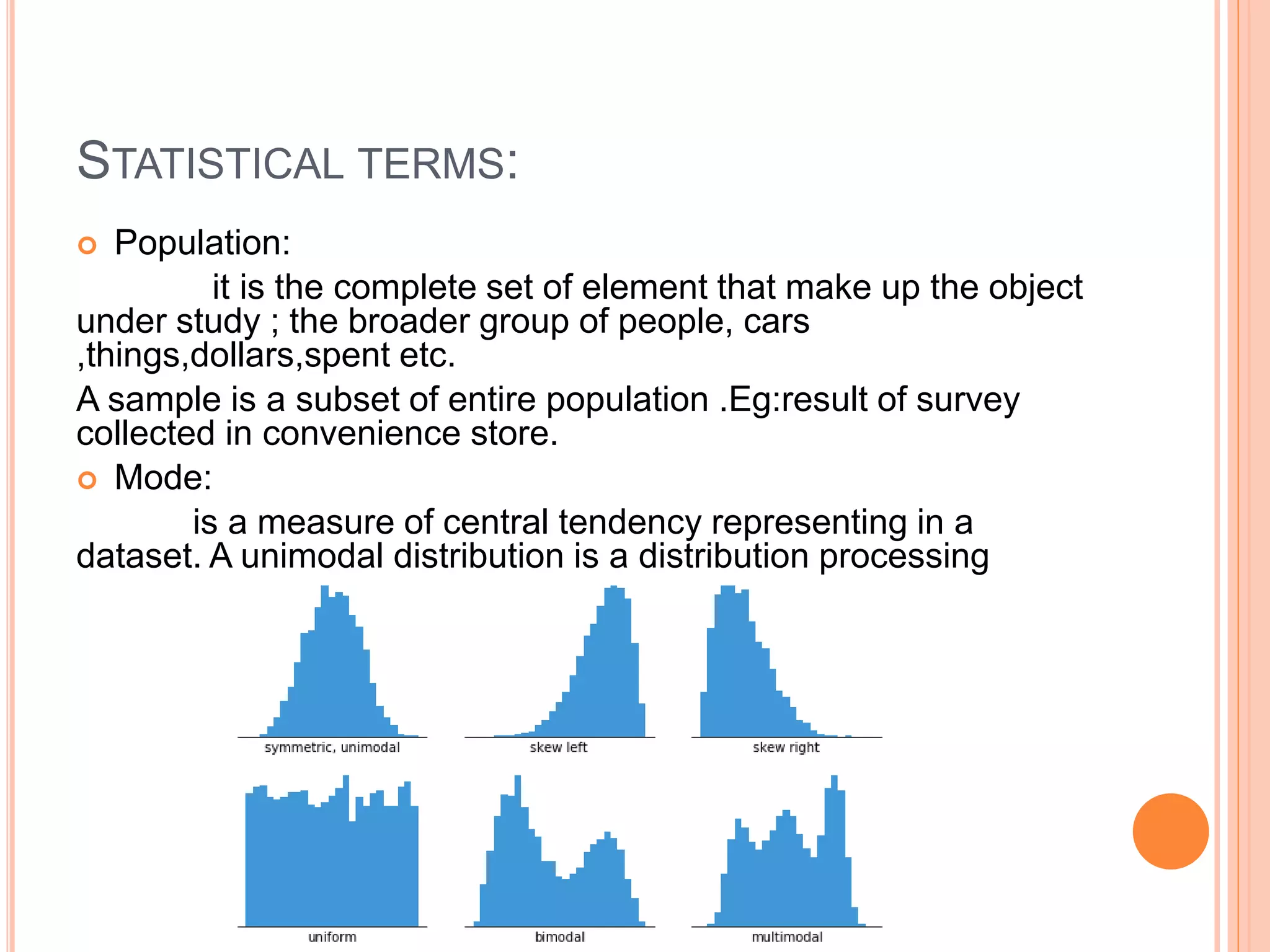
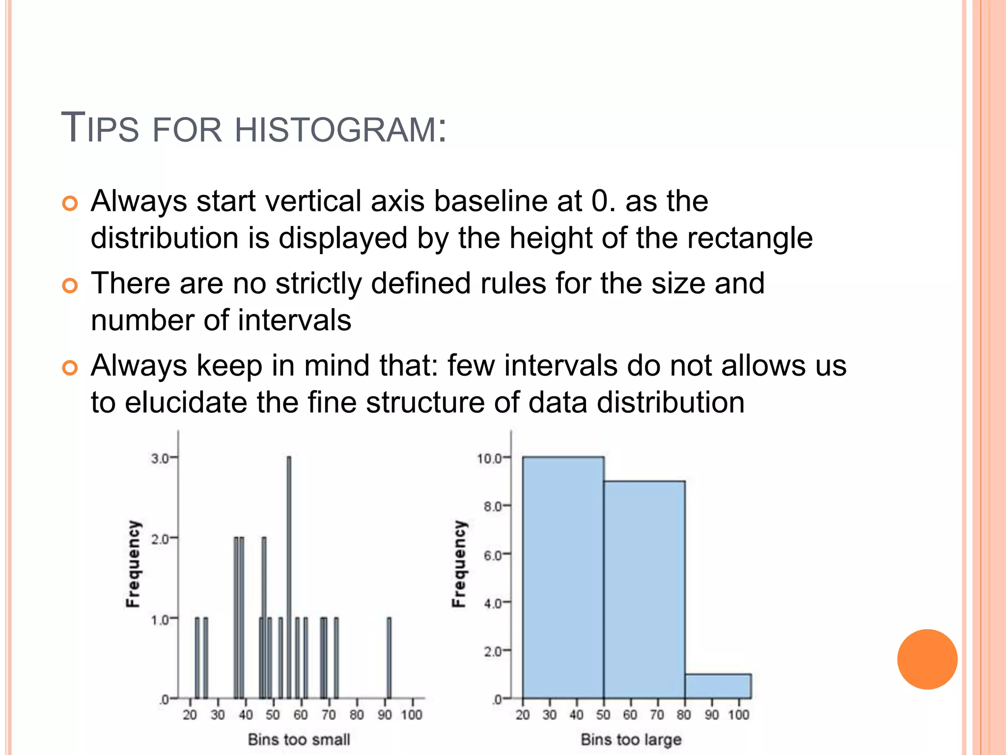
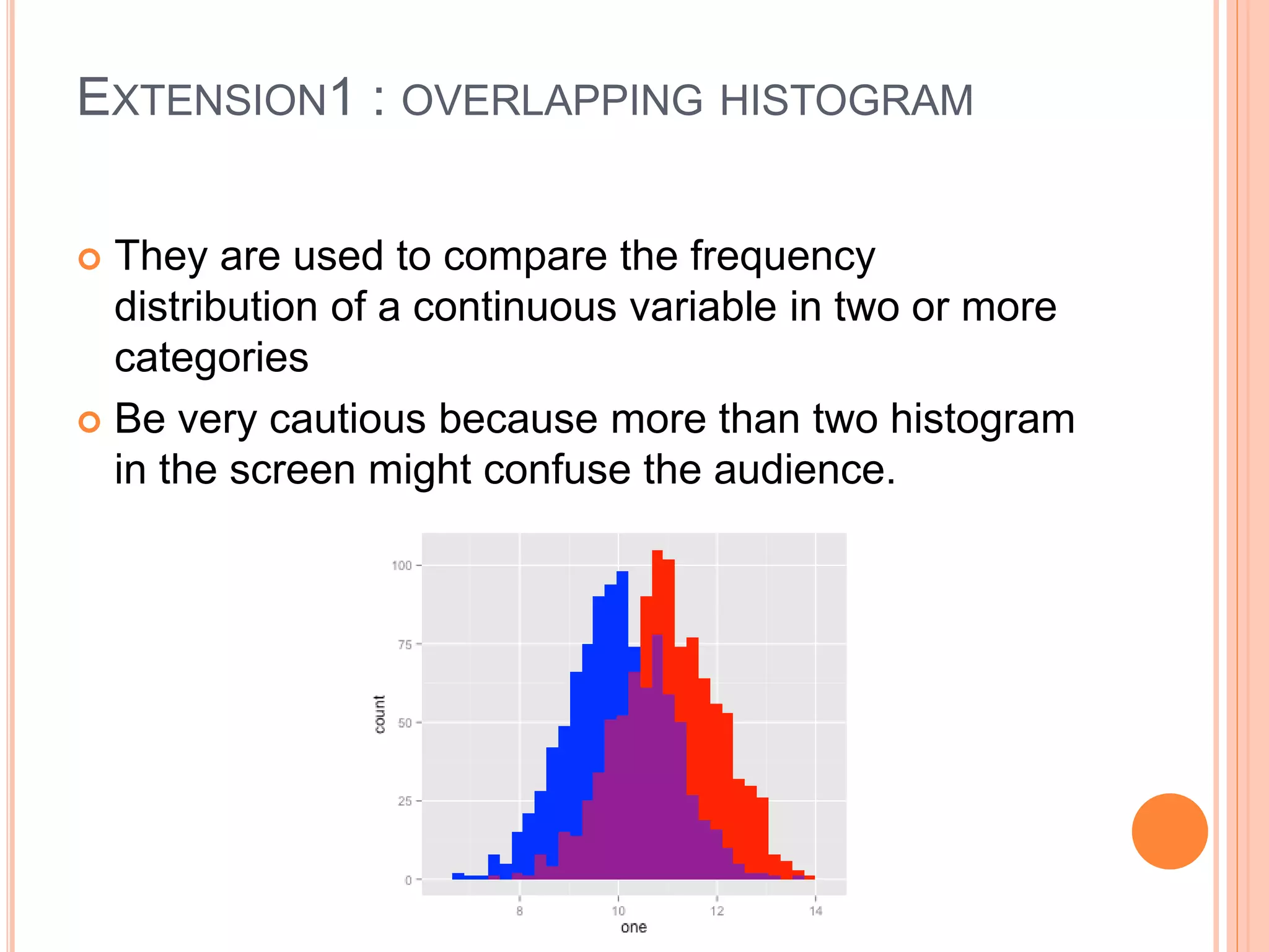
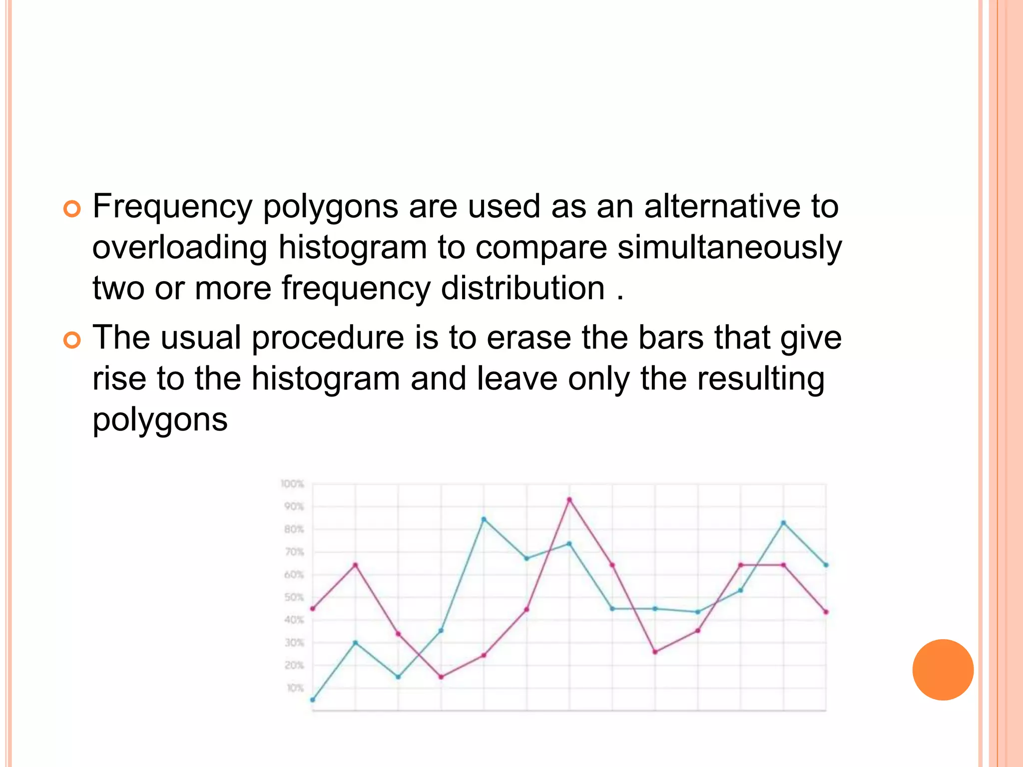
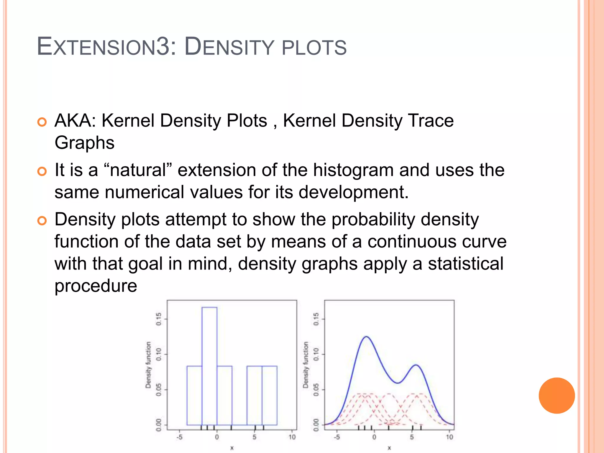
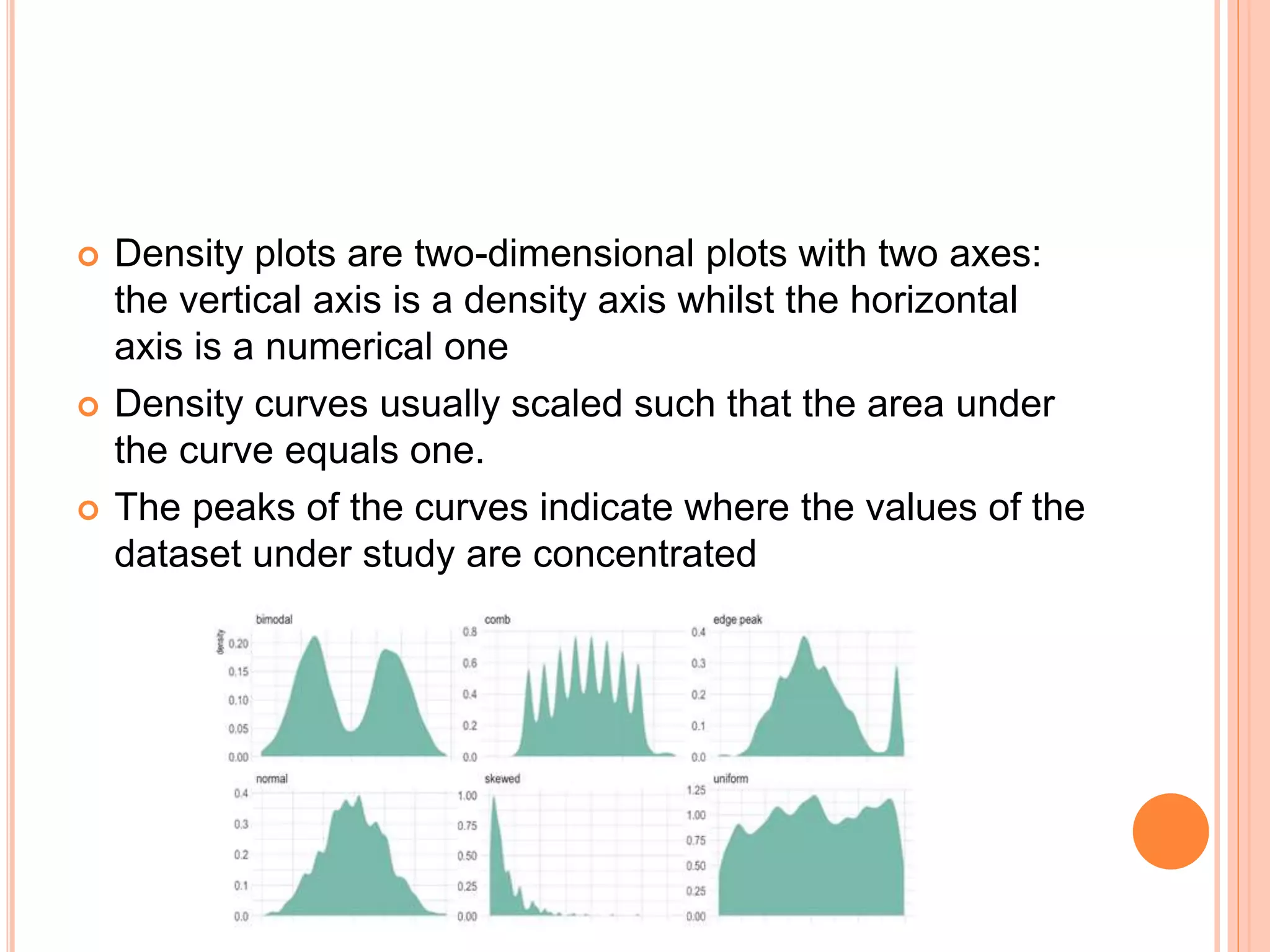
Plotting histogram in bigdata analytics

Plotting histogram in bigdata analytics

• 1.
  PLOTTING HISTOGRAM INBIG DATA ANALYTICS by., K.RAJALAKSHMI II-MSC(IT) Department of CS&IT Nadar saraswathi college of arts and science,theni
• 2.
  SYNOPSIS:  Introduction  HowHistogram works  Schematic diagram  Storytelling  Statistical terms  Tips for histogram  DW HG & BC  Extension1 : overlapping histogram  Exension2: Frequency polygon  Extension3: Density plots
• 3.
  INTRODUCTION:  A histogramis a graphical representation of the distribution of a dataset.  Although its appearance is similar to that of a standard bar graph , instead of making comparisons between different items or categories trends over time , a histogram is plot that lets show probability distribution of a single continuous numerical variable Column histogram 
• 4.
  HOW HISTOGRAM WORKS: Histogram are two-dimensional plots with two axes; the vertical axis is a frequency axis whilst the horizontal axis is divided into a range of numeric values or time intervals .  The frequency of each bin is shown by the area of vertical rectangular bars  Histogram sometimes have bars of unequal width  Collect data from individuals in a population, split the data between bins of 10 years age ranges but accumulation in a single interval data from people over 75 years old binwidth is same for all intervals replace bar area with bar length.
• 5.
  SCHEMATIC DIAGRAM:  Ahistogram shows the frequency distribution that is used to represent the probability distribution of a single continuous quantitative variables  It id not height but the area of the rectangle which is proportional of each range of values in which continuous variable is divided
• 6.
  STORYTELLING:  A histogramis the appropriate graph for the initial exploration of a continuous variable.  By means of a set of vertical bars , it shows how the numerical values of that variable are distributed .  The histogram allows to calculate the probability of representation of any value of the continuous variable  A histogram provides a visual representation of the distribution of a data set : location, spread and skewers of the data  in addition if it is unimodal, bimodal or multimodal
• 7.
  STATISTICAL TERMS:  Population: itis the complete set of element that make up the object under study ; the broader group of people, cars ,things,dollars,spent etc. A sample is a subset of entire population .Eg:result of survey collected in convenience store.  Mode: is a measure of central tendency representing in a dataset. A unimodal distribution is a distribution processing
• 8.
  TIPS FOR HISTOGRAM: Always start vertical axis baseline at 0. as the distribution is displayed by the height of the rectangle  There are no strictly defined rules for the size and number of intervals  Always keep in mind that: few intervals do not allows us to elucidate the fine structure of data distribution
• 9.
  DW HG &BC:  Standard bar chats are used to make numerical comparison amongst categories whilst histogram are used to show frequency distribution of a dataset;  BCs plots categories while HGs graphs quantitative data grouped into intervals;  There are no “gaps” spaces between the bars of a histogram; it is mandatory to leave some space between the bars on a BC to clearly indicate that it refers to discrete groups  All bars in a BC must have same width. Histogram may have bars with different width.
• 10.
  EXTENSION1 : OVERLAPPINGHISTOGRAM  They are used to compare the frequency distribution of a continuous variable in two or more categories  Be very cautious because more than two histogram in the screen might confuse the audience.
• 11.
  EXENSION2: FREQUENCY POLYGON It is a graph derived from a typical histogram.  It consists of connected line segments formed by joining the midpoints of the upper edges of the histogram’s bar.  All bars in a frequency polygon must have the same width
• 12.
   Frequency polygonsare used as an alternative to overloading histogram to compare simultaneously two or more frequency distribution .  The usual procedure is to erase the bars that give rise to the histogram and leave only the resulting polygons
• 13.
  EXTENSION3: DENSITY PLOTS AKA: Kernel Density Plots , Kernel Density Trace Graphs  It is a “natural” extension of the histogram and uses the same numerical values for its development.  Density plots attempt to show the probability density function of the data set by means of a continuous curve with that goal in mind, density graphs apply a statistical procedure
• 14.
   Density plotsare two-dimensional plots with two axes: the vertical axis is a density axis whilst the horizontal axis is a numerical one  Density curves usually scaled such that the area under the curve equals one.  The peaks of the curves indicate where the values of the dataset under study are concentrated
• 15.
  THANK YOU