Downloaded 36 times

![Pointer Jumping –list ranking
Given a single linked list L with n objects,
compute, for each object in L, its distance from the
end of the list.
Formally: suppose next is the pointer field
d[i]= 0 if next[i]=nil
d[next[i]]+1 if next[i]≠nil
Serial algorithm: Θ(n).
5](https://image.slidesharecdn.com/parallelalgorithms-171108090051/75/Parallel-algorithms-5-2048.jpg)
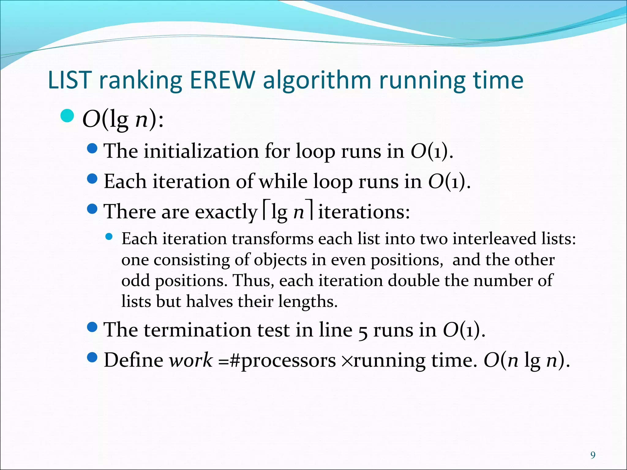
![List ranking –EREW algorithm
LIST-RANK(L) (in O(lg n) time)
1. for each processor i, in parallel
2. do if next[i]=nil
3. then d[i]←0
4. else d[i]←1
5. while there exists an object i such that next[i]≠nil
6. do for each processor i, in parallel
7. do if next[i]≠nil
8. then d[i]← d[i]+ d[next[i]]
9. next[i] ←next[next[i]]
6](https://image.slidesharecdn.com/parallelalgorithms-171108090051/75/Parallel-algorithms-6-2048.jpg)
![List ranking –correctness of EREW algorithm
Loop invariant: for each i, the sum of d values
in the sublist headed by i is the correct
distance from i to the end of the original list L.
Parallel memory must be synchronized: the
reads on the right must occur before the wirtes
on the left. Moreover, read d[i] and then read
d[next[i]].
An EREW algorithm: every read and write is
exclusive. For an object i, its processor reads
d[i], and then its precedent processor reads its
d[i]. Writes are all in distinct locations.
8](https://image.slidesharecdn.com/parallelalgorithms-171108090051/75/Parallel-algorithms-8-2048.jpg)
![Parallel prefix on a list
A prefix computation is defined as:
Input: <x1, x2, …, xn>
Binary associative operation ⊗
Output:<y1, y2, …, yn>
Such that:
y1= x1
yk= yk-1⊗ xkfork=2,3, …,n, i.e, yk= ⊗ x1⊗ x2 …⊗ xk.
Suppose <x1, x2, …, xn> are stored orderly in a list.
Define notation: [i,j]= xi⊗ xi+1 …⊗ xj
10](https://image.slidesharecdn.com/parallelalgorithms-171108090051/75/Parallel-algorithms-10-2048.jpg)
![Prefix computation LIST-PREFIX(L)
1. for each processor i, in parallel
2. do y[i]← x[i]
3. while there exists an object i such that next[i]≠nil
4. do for each processor i, in parallel
5. do if next[i]≠nil
6. then y[next[i]]← y[i] ⊗ y[next[i]]
7. next[i] ←next[next[i]]
11](https://image.slidesharecdn.com/parallelalgorithms-171108090051/75/Parallel-algorithms-11-2048.jpg)
![12
[1,1]
x1
[2,2]
x2
[3,3] [4,4]
x4
[5,5]
x5
[6,6]
x6
(a)
x3
x4
(b)
x1 x2 x5
x6x3
[1,1] [1,2] [2,3] [3,4] [4,5] [5,6]
x1 x2 x5
x6x3
x1 x2 x5
x6x3
(c)
(d)
[1,1] [1,2] [1,3] [1,4] [2,5] [3,6]
[1,1] [1,2] [1,3] [1,4] [1,5] [1,6]](https://image.slidesharecdn.com/parallelalgorithms-171108090051/75/Parallel-algorithms-12-2048.jpg)
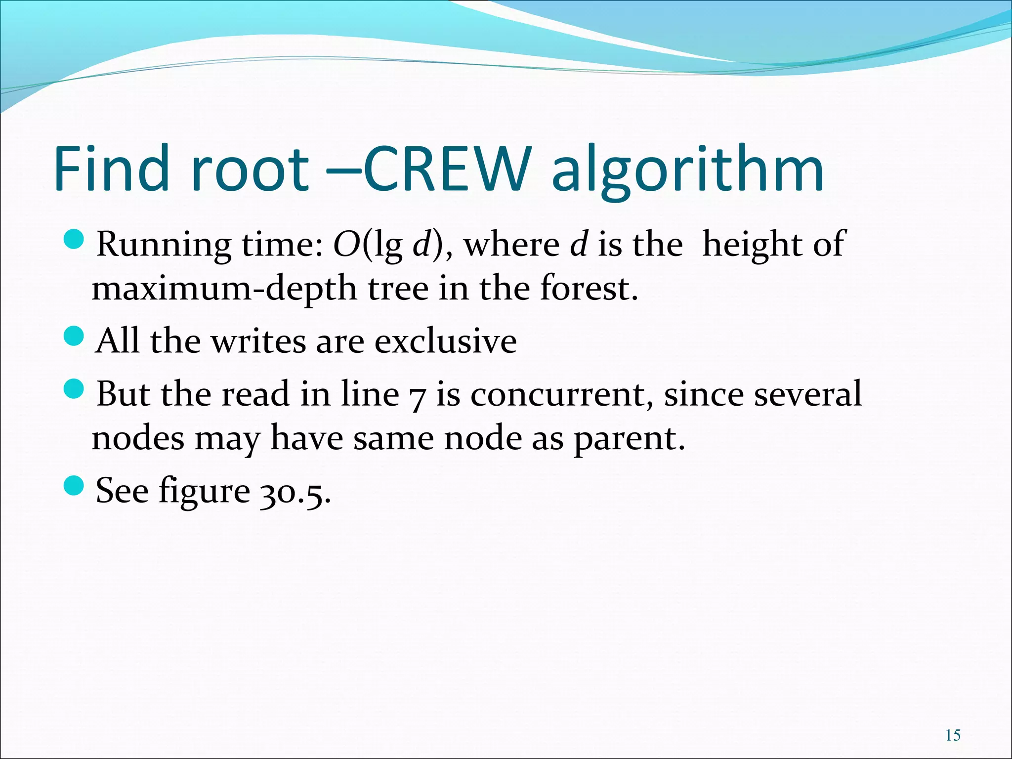
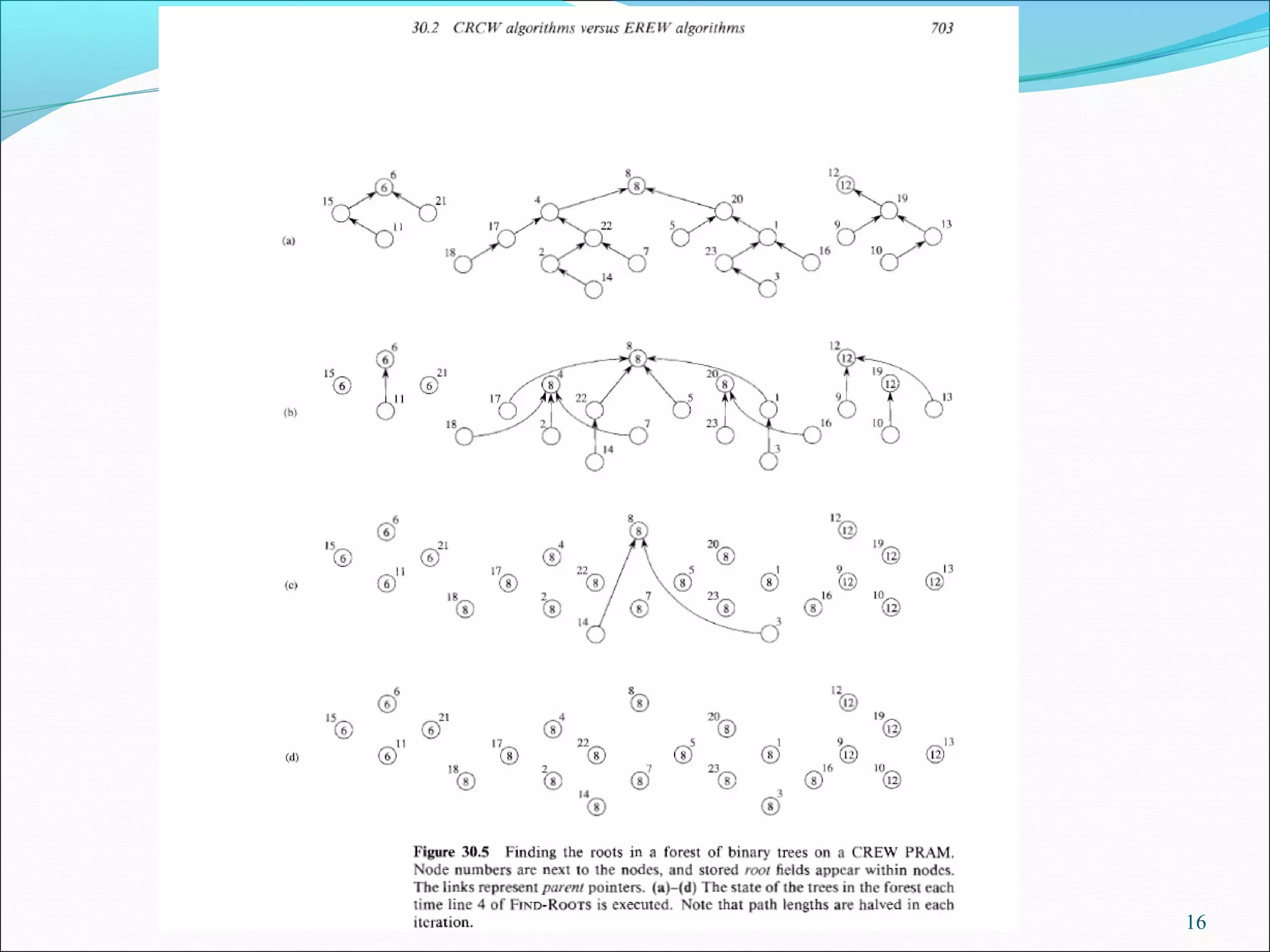
![Find root –CREW algorithm
Suppose a forest of binary trees, each node i has a
pointer parent[i].
Find the identity of the tree of each node.
Assume that each node is associated a processor.
Assume that each node i has a field root[i].
13](https://image.slidesharecdn.com/parallelalgorithms-171108090051/75/Parallel-algorithms-13-2048.jpg)
![Find-roots –CREW algorithm
FIND-ROOTS(F)
1. for each processor i, in parallel
2. do if parent[i] = nil
3. then root[i]←i
4. while there exist a node i such that parent[i] ≠ nil
5. do for each processor i, in parallel
6. do if parent[i] ≠ nil
7. then root[i] ← root[parent[i]]
8. parent[i] ← parent[parent[i]]
14](https://image.slidesharecdn.com/parallelalgorithms-171108090051/75/Parallel-algorithms-14-2048.jpg)
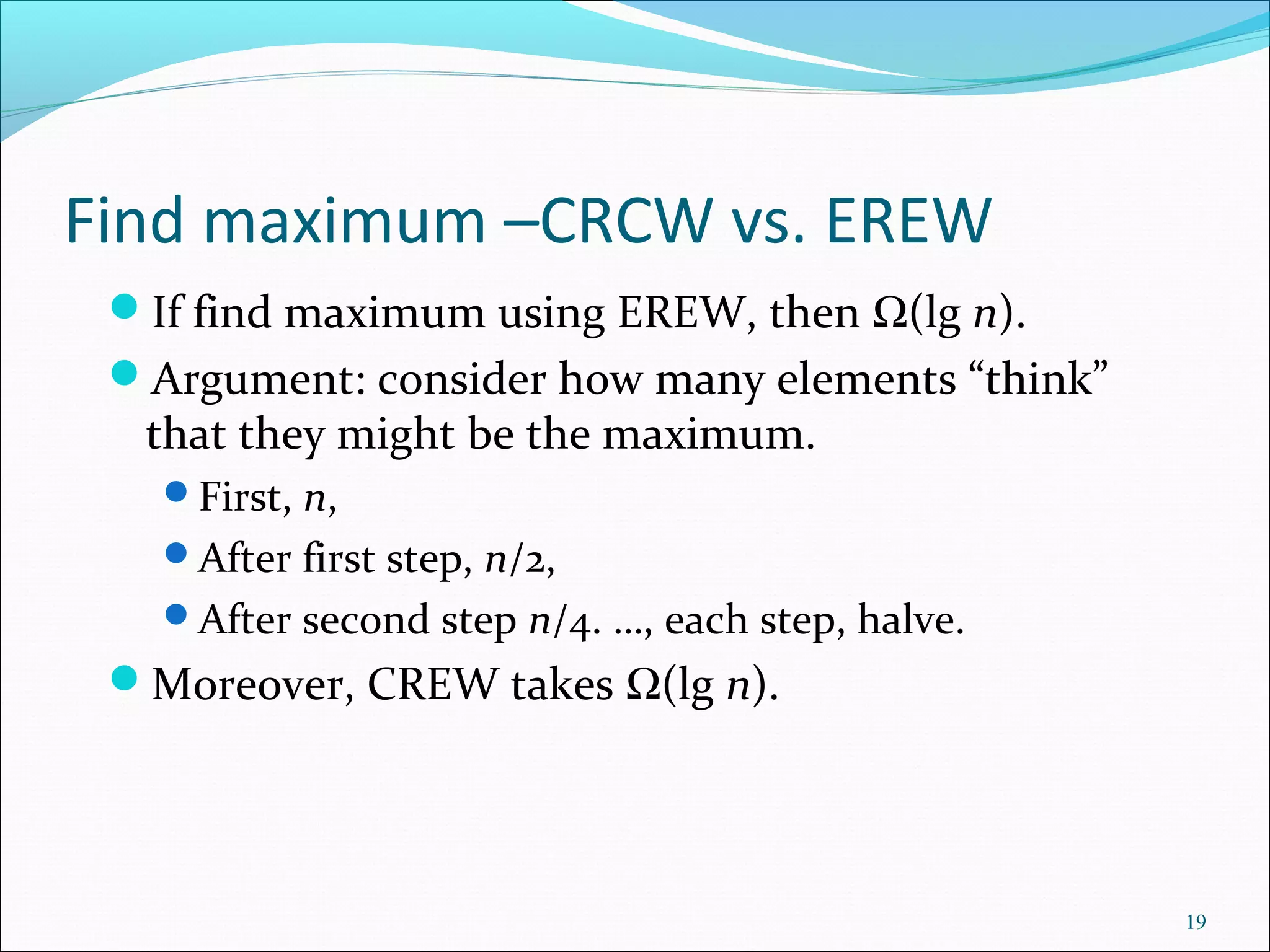
![Find maximum – CRCW algorithm Given n elements A[0,n-1], find the maximum.
Suppose n2
processors, each processor (i,j) compare A[i] and A[j], for 0≤
i, j ≤n-1.
FAST-MAX(A)
1. n←length[A]
2. for i ←0 to n-1, in parallel
3. do m[i] ←true
4. for i ←0 to n-1 and j ←0 to n-1, in parallel
5. do if A[i] < A[j]
6. then m[i] ←false
7. for i ←0 to n-1, in parallel
8. do if m[i] =true
9. then max ← A[i]
10. return max
18
The running time is O(1).
Note: there may be multiple maximum values, so their processors
Will write to max concurrently. Its work = n2
× O(1) =O(n2
).
5 6 9 2 9 m
5 F T T F T F
6 F F T F T F
9 F F F F F T
2 T T T F T F
9 F F F F F T
A[j]
A[i]
max=9](https://image.slidesharecdn.com/parallelalgorithms-171108090051/75/Parallel-algorithms-18-2048.jpg)
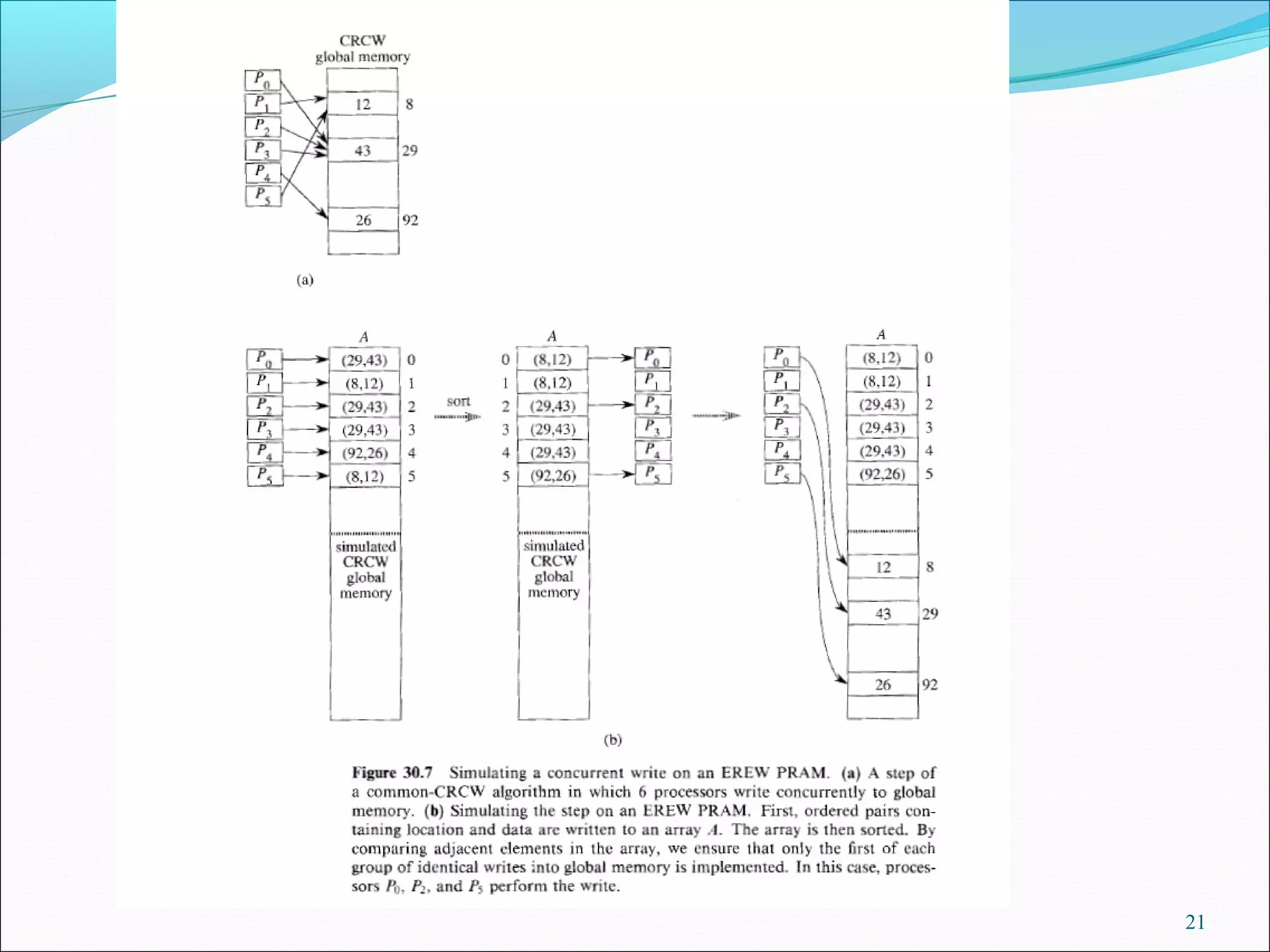
![Stimulating CRCW with EREW
Theorem:
A p-processor CRCW algorithm can be no more than O(lg p)
times faster than a best p-processor EREW algorithm for the same
problem.
Proof: each step of CRCW can be simulated by O(lg p)
computations of EREW.
Suppose concurrent write:
CRCW pi write data xi to location li, (li may be same for multiple pi ‘s).
Corresponding EREW pi write (li, xi) to a location A[i], (different A[i]’s)
so exclusive write.
Sort all (li, xi)’s by li’s, same locations are brought together. in O(lg p).
Each EREW picompares A[i]= (lj, xj), and A[i-1]= (lk, xk). If lj≠ lk or i=0,
then EREW pi writes xj to lj. (exclusive write).
See figure 30.7.
20](https://image.slidesharecdn.com/parallelalgorithms-171108090051/75/Parallel-algorithms-20-2048.jpg)


![Pointer Jumping –list ranking
Given a single linked list L with n objects,
compute, for each object in L, its distance from the
end of the list.
Formally: suppose next is the pointer field
d[i]= 0 if next[i]=nil
d[next[i]]+1 if next[i]≠nil
Serial algorithm: Θ(n).
5](https://crownmelresort.com/image.slidesharecdn.com/parallelalgorithms-171108090051/75/Parallel-algorithms-5-2048.jpg)
![List ranking –EREW algorithm
LIST-RANK(L) (in O(lg n) time)
1. for each processor i, in parallel
2. do if next[i]=nil
3. then d[i]←0
4. else d[i]←1
5. while there exists an object i such that next[i]≠nil
6. do for each processor i, in parallel
7. do if next[i]≠nil
8. then d[i]← d[i]+ d[next[i]]
9. next[i] ←next[next[i]]
6](https://crownmelresort.com/image.slidesharecdn.com/parallelalgorithms-171108090051/75/Parallel-algorithms-6-2048.jpg)

![List ranking –correctness of EREW algorithm
Loop invariant: for each i, the sum of d values
in the sublist headed by i is the correct
distance from i to the end of the original list L.
Parallel memory must be synchronized: the
reads on the right must occur before the wirtes
on the left. Moreover, read d[i] and then read
d[next[i]].
An EREW algorithm: every read and write is
exclusive. For an object i, its processor reads
d[i], and then its precedent processor reads its
d[i]. Writes are all in distinct locations.
8](https://crownmelresort.com/image.slidesharecdn.com/parallelalgorithms-171108090051/75/Parallel-algorithms-8-2048.jpg)

![Parallel prefix on a list
A prefix computation is defined as:
Input: <x1, x2, …, xn>
Binary associative operation ⊗
Output:<y1, y2, …, yn>
Such that:
y1= x1
yk= yk-1⊗ xkfork=2,3, …,n, i.e, yk= ⊗ x1⊗ x2 …⊗ xk.
Suppose <x1, x2, …, xn> are stored orderly in a list.
Define notation: [i,j]= xi⊗ xi+1 …⊗ xj
10](https://crownmelresort.com/image.slidesharecdn.com/parallelalgorithms-171108090051/75/Parallel-algorithms-10-2048.jpg)
![Prefix computation LIST-PREFIX(L)
1. for each processor i, in parallel
2. do y[i]← x[i]
3. while there exists an object i such that next[i]≠nil
4. do for each processor i, in parallel
5. do if next[i]≠nil
6. then y[next[i]]← y[i] ⊗ y[next[i]]
7. next[i] ←next[next[i]]
11](https://crownmelresort.com/image.slidesharecdn.com/parallelalgorithms-171108090051/75/Parallel-algorithms-11-2048.jpg)
![12
[1,1]
x1
[2,2]
x2
[3,3] [4,4]
x4
[5,5]
x5
[6,6]
x6
(a)
x3
x4
(b)
x1 x2 x5
x6x3
[1,1] [1,2] [2,3] [3,4] [4,5] [5,6]
x1 x2 x5
x6x3
x1 x2 x5
x6x3
(c)
(d)
[1,1] [1,2] [1,3] [1,4] [2,5] [3,6]
[1,1] [1,2] [1,3] [1,4] [1,5] [1,6]](https://crownmelresort.com/image.slidesharecdn.com/parallelalgorithms-171108090051/75/Parallel-algorithms-12-2048.jpg)
![Find root –CREW algorithm
Suppose a forest of binary trees, each node i has a
pointer parent[i].
Find the identity of the tree of each node.
Assume that each node is associated a processor.
Assume that each node i has a field root[i].
13](https://crownmelresort.com/image.slidesharecdn.com/parallelalgorithms-171108090051/75/Parallel-algorithms-13-2048.jpg)
![Find-roots –CREW algorithm
FIND-ROOTS(F)
1. for each processor i, in parallel
2. do if parent[i] = nil
3. then root[i]←i
4. while there exist a node i such that parent[i] ≠ nil
5. do for each processor i, in parallel
6. do if parent[i] ≠ nil
7. then root[i] ← root[parent[i]]
8. parent[i] ← parent[parent[i]]
14](https://crownmelresort.com/image.slidesharecdn.com/parallelalgorithms-171108090051/75/Parallel-algorithms-14-2048.jpg)


![Find maximum – CRCW algorithm Given n elements A[0,n-1], find the maximum.
Suppose n2
processors, each processor (i,j) compare A[i] and A[j], for 0≤
i, j ≤n-1.
FAST-MAX(A)
1. n←length[A]
2. for i ←0 to n-1, in parallel
3. do m[i] ←true
4. for i ←0 to n-1 and j ←0 to n-1, in parallel
5. do if A[i] < A[j]
6. then m[i] ←false
7. for i ←0 to n-1, in parallel
8. do if m[i] =true
9. then max ← A[i]
10. return max
18
The running time is O(1).
Note: there may be multiple maximum values, so their processors
Will write to max concurrently. Its work = n2
× O(1) =O(n2
).
5 6 9 2 9 m
5 F T T F T F
6 F F T F T F
9 F F F F F T
2 T T T F T F
9 F F F F F T
A[j]
A[i]
max=9](https://crownmelresort.com/image.slidesharecdn.com/parallelalgorithms-171108090051/75/Parallel-algorithms-18-2048.jpg)

![Stimulating CRCW with EREW
Theorem:
A p-processor CRCW algorithm can be no more than O(lg p)
times faster than a best p-processor EREW algorithm for the same
problem.
Proof: each step of CRCW can be simulated by O(lg p)
computations of EREW.
Suppose concurrent write:
CRCW pi write data xi to location li, (li may be same for multiple pi ‘s).
Corresponding EREW pi write (li, xi) to a location A[i], (different A[i]’s)
so exclusive write.
Sort all (li, xi)’s by li’s, same locations are brought together. in O(lg p).
Each EREW picompares A[i]= (lj, xj), and A[i-1]= (lk, xk). If lj≠ lk or i=0,
then EREW pi writes xj to lj. (exclusive write).
See figure 30.7.
20](https://crownmelresort.com/image.slidesharecdn.com/parallelalgorithms-171108090051/75/Parallel-algorithms-20-2048.jpg)


This document discusses parallel algorithms and models of parallel computation. It begins with an overview of parallelism and the PRAM model of computation. It then discusses different models of concurrent versus exclusive access to shared memory. Several parallel algorithms are presented, including list ranking in O(log n) time using an EREW PRAM algorithm and finding the maximum of n elements in O(1) time using a CRCW PRAM algorithm. It analyzes the performance of EREW versus CRCW models and shows how to simulate a CRCW algorithm using EREW in O(log p) time using p processors.
Introduction to the concept of parallel algorithms by Shashikant V. Athawale, who is an Assistant Professor in Computer Engineering.
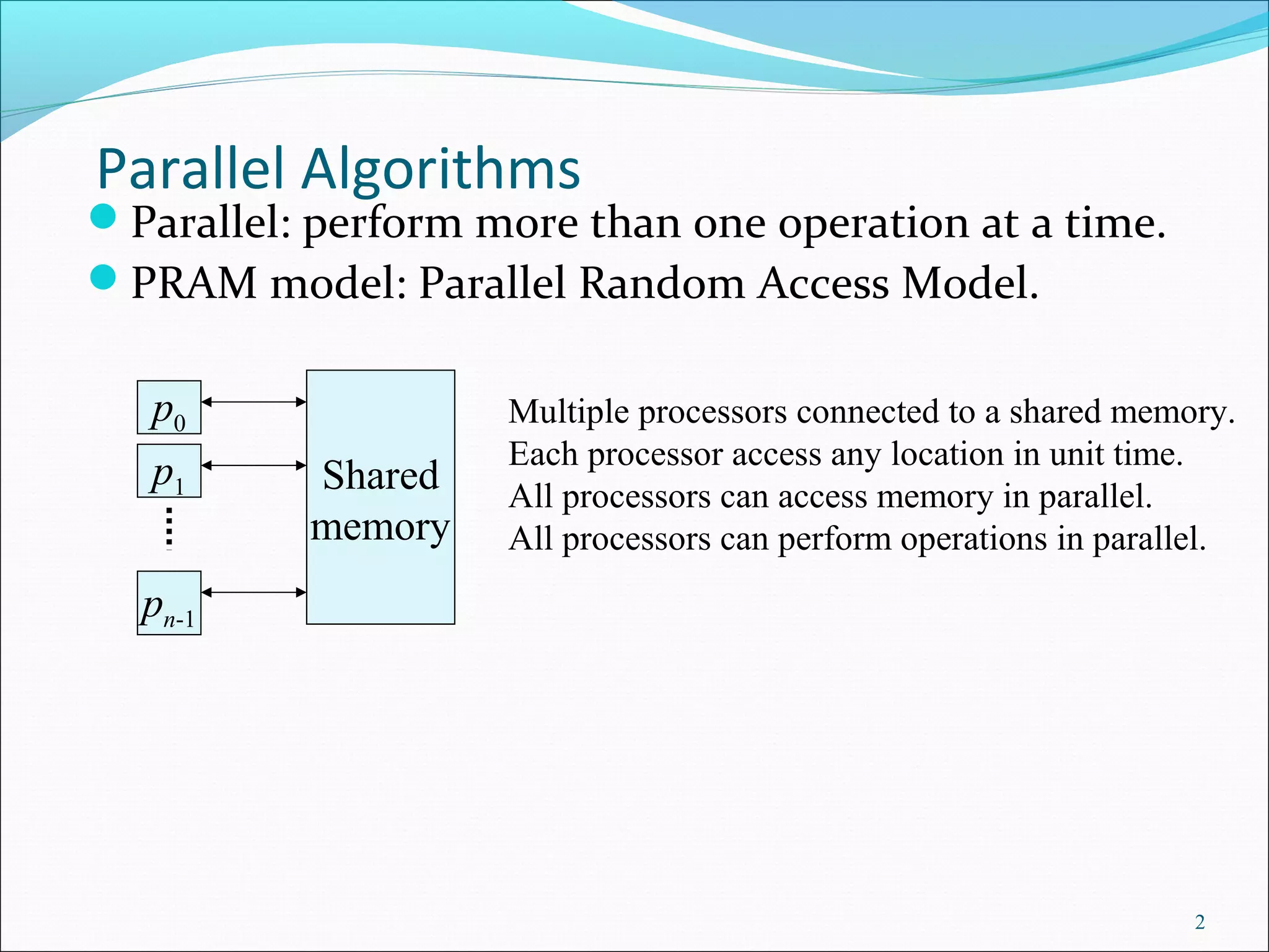
Outline of parallelism, defining a PRAM model with shared memory and operation capabilities for multiple processors.
Four access models (EREW, CREW, ERCW, CRCW) for concurrent and exclusive operations; describes handling write conflicts.
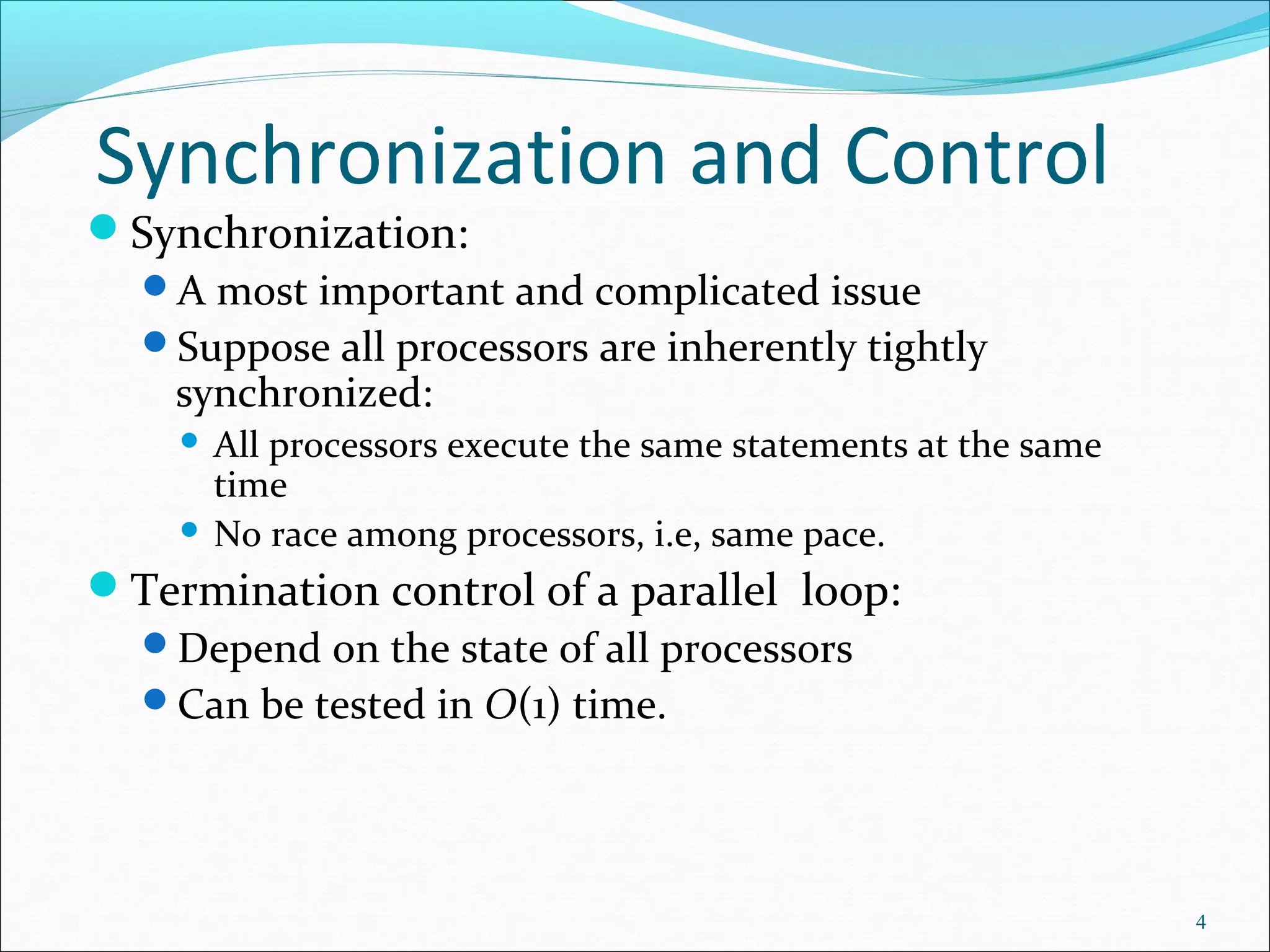
Explains synchronization issues in parallel algorithms and discusses termination control in parallel loops.
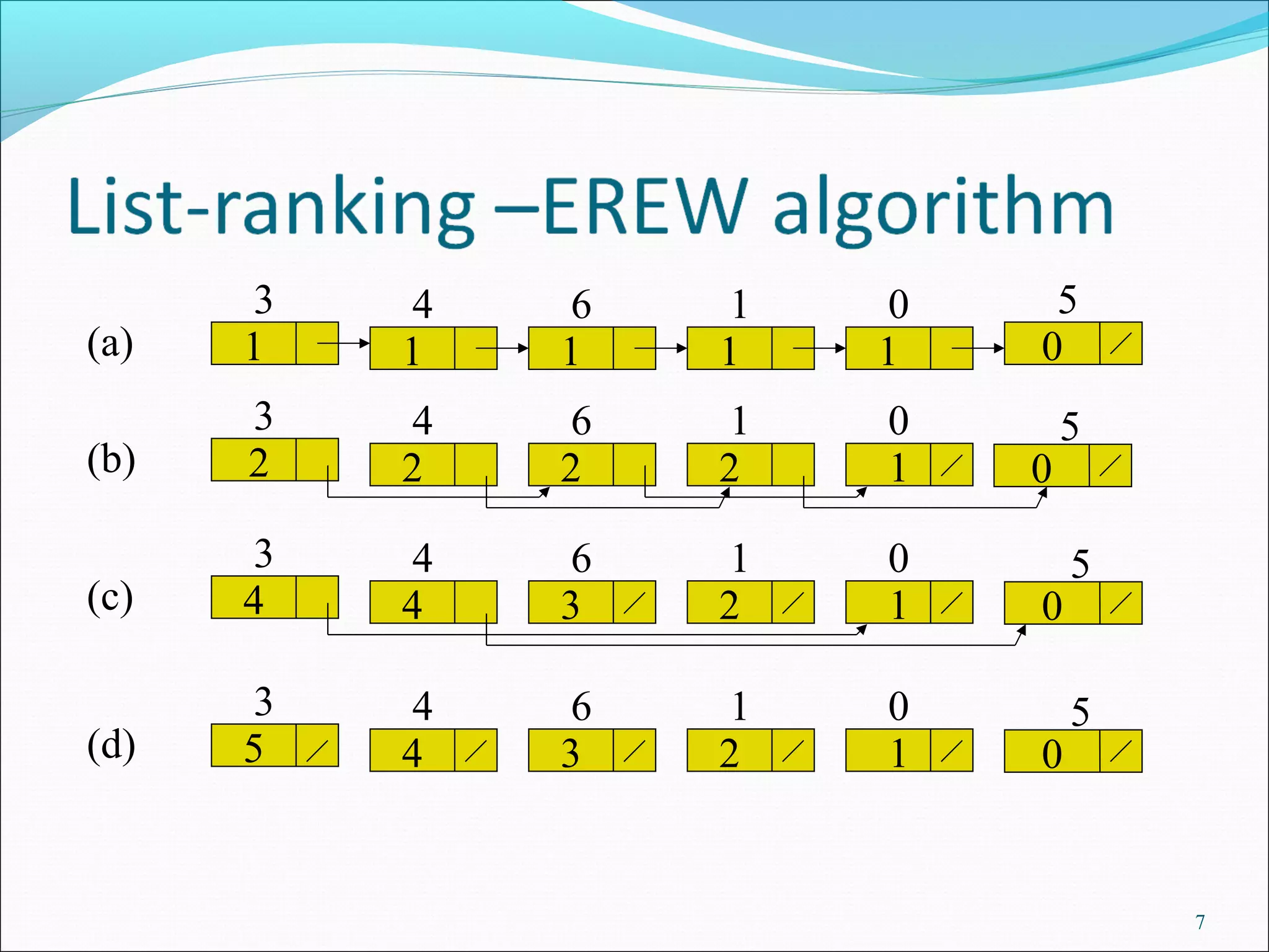
Description of the pointer jumping method for list ranking, calculating distances of linked list objects.
Algorithm outline for LIST-RANK using EREW model to compute distances in a linked list in parallel.
Illustrations showing steps and results of the LIST-RANK algorithm with various data outcomes.
Discussion on the correctness of the EREW algorithm with emphasis on loop invariants and memory synchronization.
Analysis of running time for LIST-RANK EREW algorithm, calculating complexity in terms of work and iterations.
Introduction to prefix computation defined with input, binary associative operation, and the expected output.
Algorithm for LIST-PREFIX using parallel processing to perform prefix computations on lists.
Visual representation of prefix computation stages with sequential examples shown in the slides.
Overview of the CREW approach for finding the root of nodes in a forest of binary trees using parallel processing.
Detailed execution steps of the FIND-ROOTS algorithm using CREW model for tree node processing.
Running time performance evaluation of the FIND-ROOTS algorithm, focusing on the depth of binary trees.
Comparison between CREW and EREW algorithms for finding roots, detailing their time complexities and operational differences.
Describes the CRCW algorithm to find the maximum in an array utilizing n^2 processors in parallel.
Analysis of maximum finding time complexities for EREW and CRCW algorithms, discussing their operational limits.
Theorem about CRCW simulation with EREW algorithms, discussing the implications on computational speed.
Comparative discussion on CRCW and EREW algorithms regarding programming ease, speed, and network requirements.
A closing thank you from the speaker, wrapping up the details about parallel algorithms.


![ANPARA THERMAL POWER STATION[1] sangam.pdf](https://cdn.slidesharecdn.com/ss_thumbnails/anparathermalpowerstation1sangam-251121115219-9261cde4-thumbnail.jpg?width=640&height=640&fit=bounds)


