Downloaded 141 times


![78
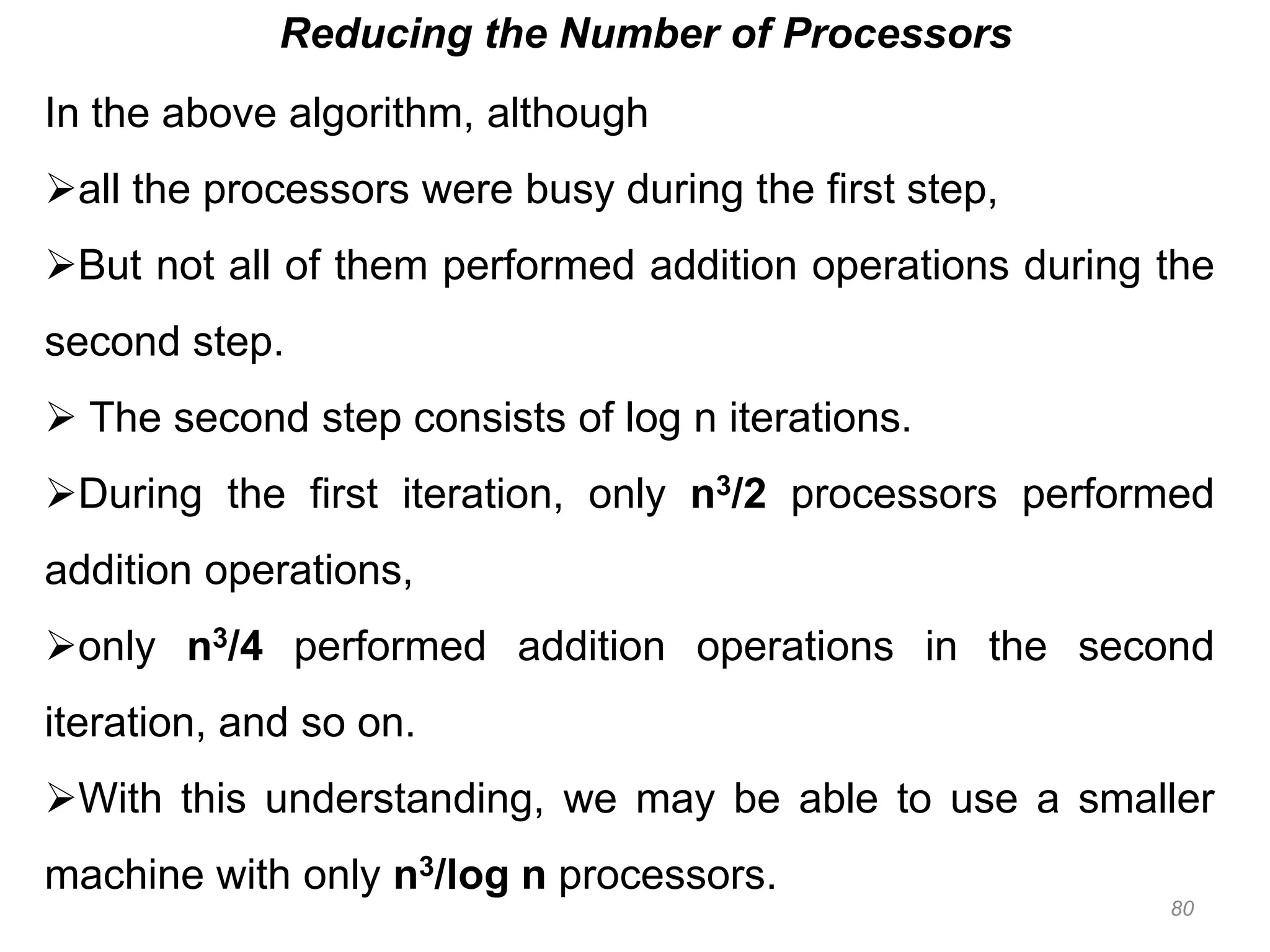
Using n3 Processors
Algorithm MatMult_CREW
/* Step 1 */
Forall Pi,j,k, where do in parallel
C[i,j,k] = A[i,k]*B[k,j]
endfor
/* Step 2 */
For I =1 to log n do
forall Pi,j,k, where do in parallel
if (2k modulo 2l)=0 then
C[i,j,2k] C[i,j,2k] + C[i,j, 2k – 2i-1]
endif
endfor
/* The output matrix is stored in locations C[i,j,n], where */
endfor](https://image.slidesharecdn.com/pa-130427003339-phpapp02/75/Parallel-Algorithms-78-2048.jpg)


![78
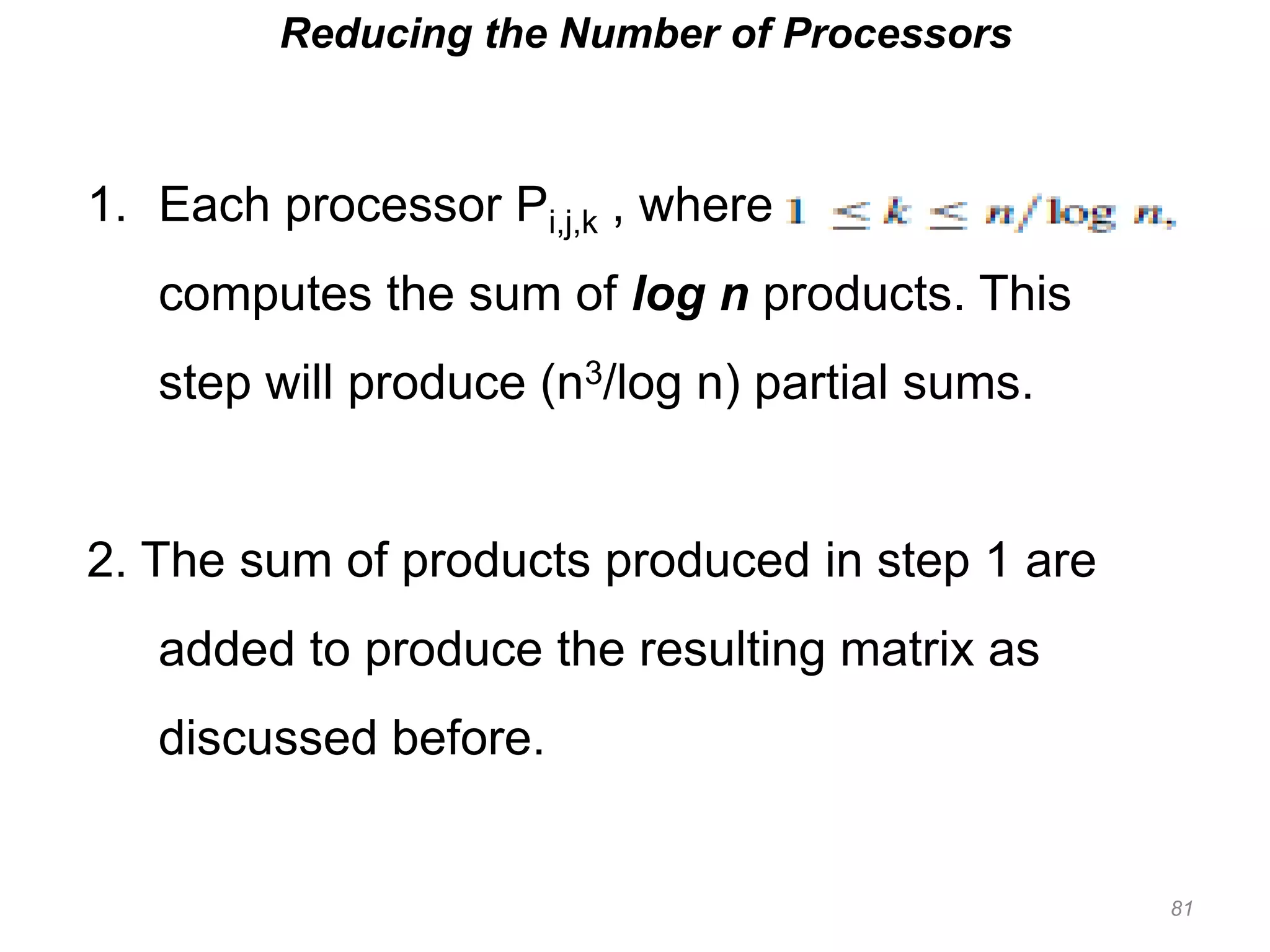
Using n3 Processors
Algorithm MatMult_CREW
/* Step 1 */
Forall Pi,j,k, where do in parallel
C[i,j,k] = A[i,k]*B[k,j]
endfor
/* Step 2 */
For I =1 to log n do
forall Pi,j,k, where do in parallel
if (2k modulo 2l)=0 then
C[i,j,2k] C[i,j,2k] + C[i,j, 2k – 2i-1]
endif
endfor
/* The output matrix is stored in locations C[i,j,n], where */
endfor](https://crownmelresort.com/image.slidesharecdn.com/pa-130427003339-phpapp02/75/Parallel-Algorithms-78-2048.jpg)


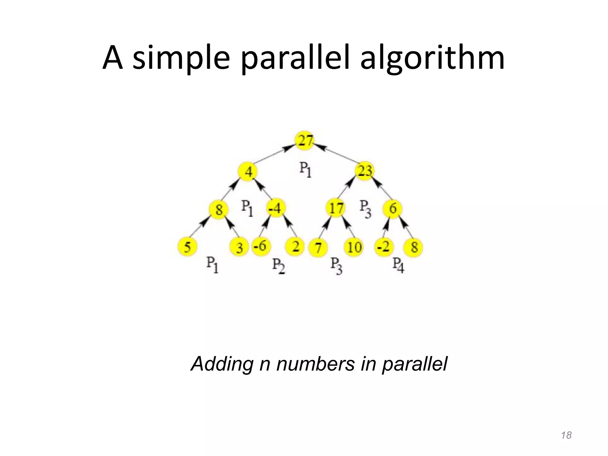
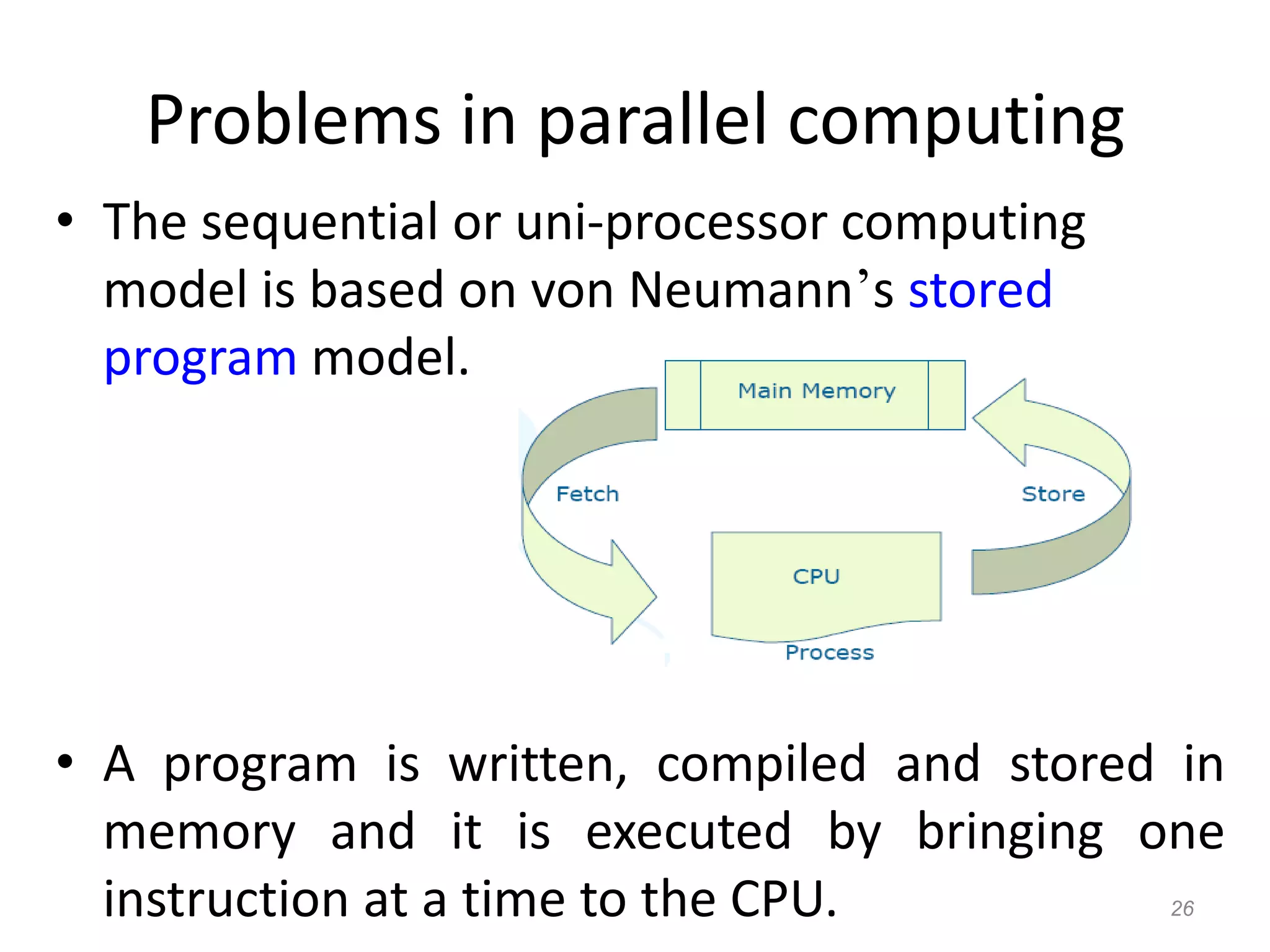
The document discusses parallel algorithms and parallel computing. It begins by defining parallelism in computers as performing more than one task at the same time. Examples of parallelism include I/O chips and pipelining of instructions. Common terms for parallelism are defined, including concurrent processing, distributed processing, and parallel processing. Issues in parallel programming such as task decomposition and synchronization are outlined. Performance issues like scalability and load balancing are also discussed. Different types of parallel machines and their classification are described.


![SHS_Core_CAE_Q3_LE1 FOR THIRD [FINAL].pdf](https://cdn.slidesharecdn.com/ss_thumbnails/shscorecaeq3le1final-251116055110-e3081055-thumbnail.jpg?width=640&height=640&fit=bounds)


