The sky over Titan’s largest colony burned with the light of Saturn’s reflection. Commander Elias Vance stood on the observation deck, gazing at the vast methane seas stretching beyond the dome’s protective barrier. The year was 2178, and humanity had long since spread beyond Earth, establishing outposts on Mars, Europa, and now, Titan. But what they found here was beyond comprehension.
It started with the signal. A faint, rhythmic pulse buried deep beneath Titan’s icy crust, repeating in a sequence no natural phenomenon could explain. The AI systems had confirmed it—this was not random. Something, or someone, was transmitting a message.
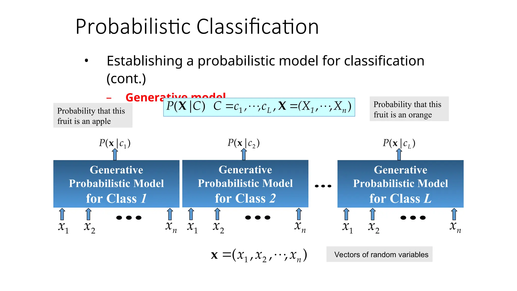

![Naïve Bayes
• Bayes classification
Bayes classification
Difficulty: learning the joint probability
• Naïve Bayes classification
Naïve Bayes classification
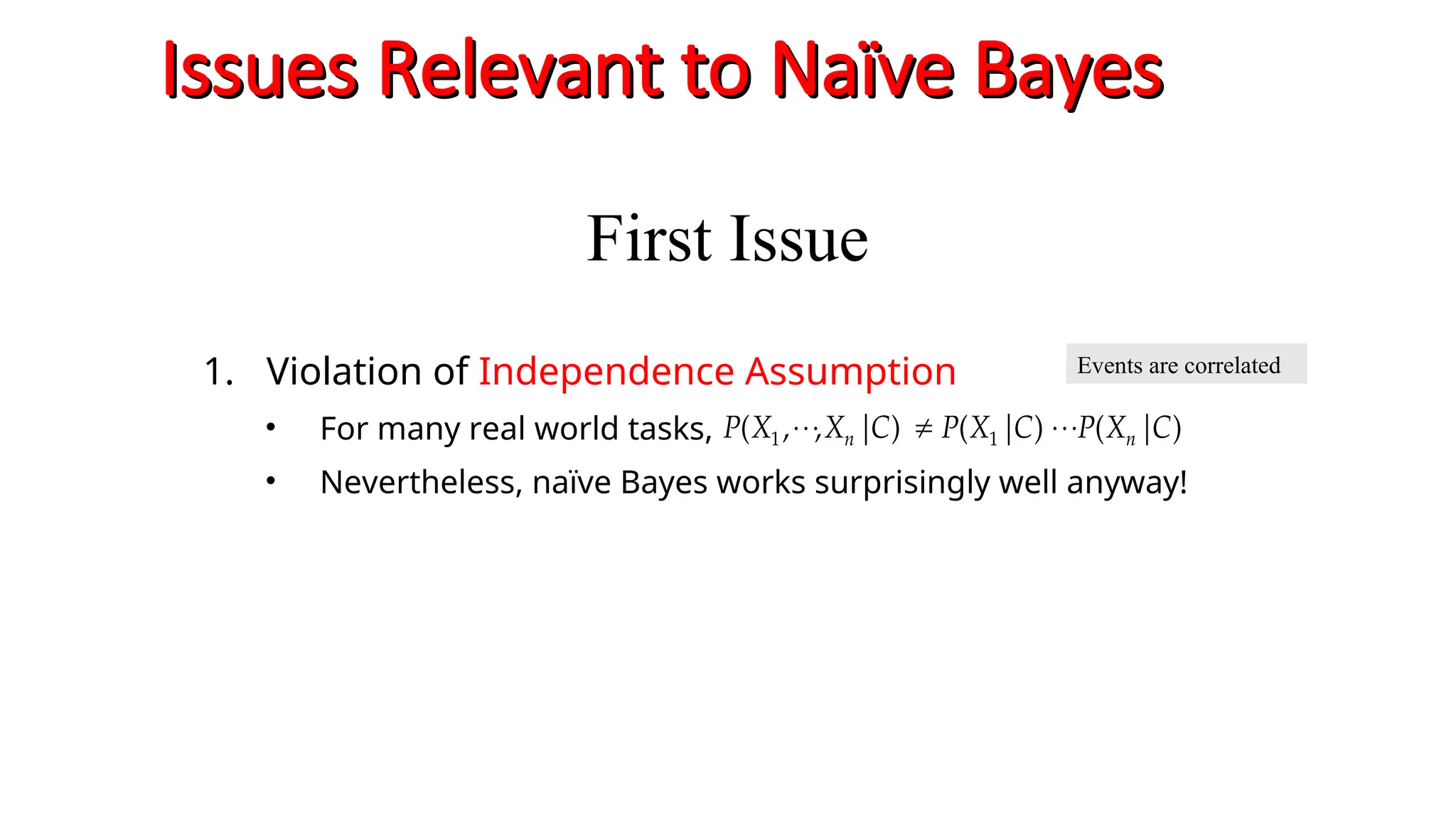
– Assumption that all input attributes are conditionally
independent!
– MAP classification rule: for
)
(
)
|
,
,
(
)
(
)
(
)
( 1 C
P
C
X
X
P
C
P
C
|
P
|
C
P n
X
X
)
|
,
,
( 1 C
X
X
P n
)
|
(
)
|
(
)
|
(
)
|
,
,
(
)
|
(
)
|
,
,
(
)
,
,
,
|
(
)
|
,
,
,
(
2
1
2
1
2
2
1
2
1
C
X
P
C
X
P
C
X
P
C
X
X
P
C
X
P
C
X
X
P
C
X
X
X
P
C
X
X
X
P
n
n
n
n
n
L
n
n c
c
c
c
c
c
P
c
x
P
c
x
P
c
P
c
x
P
c
x
P ,
,
,
),
(
)]
|
(
)
|
(
[
)
(
)]
|
(
)
|
(
[ 1
*
1
*
*
*
1
)
,
,
,
( 2
1 n
x
x
x
x
For a class, the previous generative model can be
decomposed by n
n generative models of a single
input.
Product of
individual
probabilities](https://image.slidesharecdn.com/naivebayesclassifier-250311155450-6f591eef/75/Naive-Bayes-Classifier-ppt-helping-others-by-sharing-the-ppt-10-2048.jpg)
![Naïve Bayes Algorithm
Naïve Bayes Algorithm
• Naïve Bayes Algorithm (for discrete input attributes) has two
phases
– 1. Learning Phase
1. Learning Phase: Given a training set S,
Output: conditional probability tables; for elements
– 2. Test Phase
2. Test Phase: Given an unknown instance ,
Look up tables to assign the label c* to X’ if
;
in
examples
with
)
|
(
estimate
)
|
(
ˆ
)
,
1
;
,
,
1
(
attribute
each
of
value
attribute
every
For
;
in
examples
with
)
(
estimate
)
(
ˆ
of
value
target
each
For 1
S
S
i
jk
j
i
jk
j
j
j
jk
i
i
L
i
i
c
C
x
X
P
c
C
x
X
P
N
,
k
n
j
X
x
c
C
P
c
C
P
)
c
,
,
c
(c
c
L
n
n c
c
c
c
c
c
P
c
a
P
c
a
P
c
P
c
a
P
c
a
P ,
,
,
),
(
ˆ
)]
|
(
ˆ
)
|
(
ˆ
[
)
(
ˆ
)]
|
(
ˆ
)
|
(
ˆ
[ 1
*
1
*
*
*
1
)
,
,
( 1 n
a
a
X
L
N
X j
j
,
Classification is easy, just multiply probabilities
Learning is easy, just
create probability tables.](https://image.slidesharecdn.com/naivebayesclassifier-250311155450-6f591eef/75/Naive-Bayes-Classifier-ppt-helping-others-by-sharing-the-ppt-11-2048.jpg)
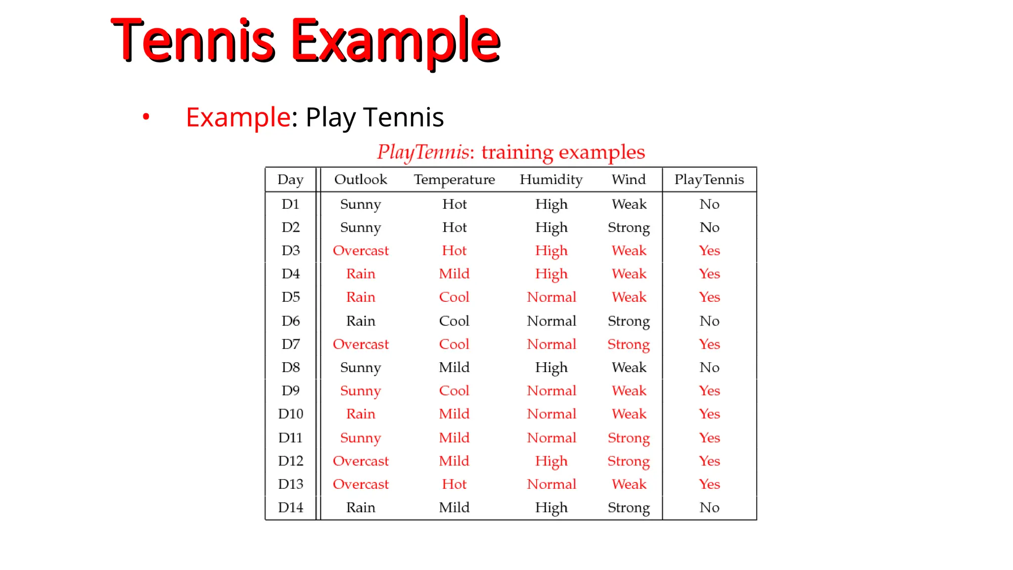
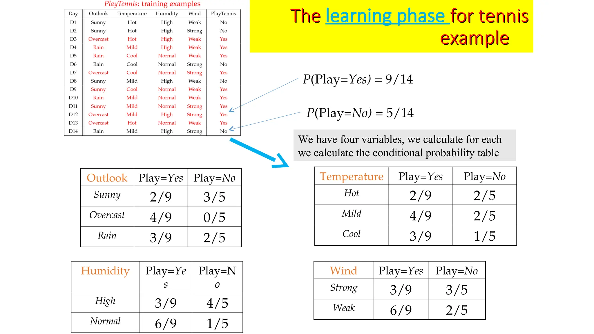
![The test phase
test phase for the tennis example
• Test Phase
– Given a new instance of variable values,
x’=(Outlook=Sunny, Temperature=Cool, Humidity=High, Wind=Strong)
– Given calculated Look up tables
– Use the
Use the MAP rule
MAP rule to calculate Yes or No
to calculate Yes or No
P(Outlook=Sunny|Play=No
No) = 3/5
P(Temperature=Cool|Play==No) = 1/5
P(Huminity=High|Play=No) = 4/5
P(Wind=Strong|Play=No) = 3/5
P(Play=No) = 5/14
P(Outlook=Sunny|Play=Yes
Yes) = 2/9
P(Temperature=Cool|Play=Yes) = 3/9
P(Huminity=High|Play=Yes) = 3/9
P(Wind=Strong|Play=Yes) = 3/9
P(Play=Yes) = 9/14
P(Yes|x’): [P(Sunny|Yes)P(Cool|Yes)P(High|Yes)P(Strong|Yes)]P(Play=Yes) = 0.0053
P(No|x’): [P(Sunny|No) P(Cool|No)P(High|No)P(Strong|No)]P(Play=No) = 0.0206
Given the fact P(
Given the fact P(Yes
Yes|
|x
x’) < P(
’) < P(No
No|
|x
x’), we label
’), we label x
x’ to be “
’ to be “No
No”.
”.](https://image.slidesharecdn.com/naivebayesclassifier-250311155450-6f591eef/75/Naive-Bayes-Classifier-ppt-helping-others-by-sharing-the-ppt-15-2048.jpg)


![• First, we apply a naïve Bayes model with 10-fold cross validation, which gets 83%
accuracy. Considering about 83% of our observations in our training set do not attrit, our
overall accuracy is no better than if we just predicted “No” attrition for every observation.
• There are several packages to apply naïve Bayes (i.e. e1071, klaR, naivebayes, bnclassify).
library(klaR)
# create response and feature data
features <- setdiff(names(train), "Attrition")
x <- train[, features]
y <- train$Attrition
# set up 10-fold cross validation procedure
train_control <- trainControl(
method = "cv",
number = 10
)
# train model
nb.m1 <- train(
x = x,
y = y,
method = "nb",
trControl = train_control
)
# results
confusionMatrix(nb.m1)
Cross-Validated (10 fold) Confusion Matrix
(entries are percentual average cell counts across resamples)
Reference
Prediction No Yes
No 75.2 8.1
Yes 8.6 8.1
Accuracy (average) : 0.833](https://image.slidesharecdn.com/naivebayesclassifier-250311155450-6f591eef/75/Naive-Bayes-Classifier-ppt-helping-others-by-sharing-the-ppt-33-2048.jpg)
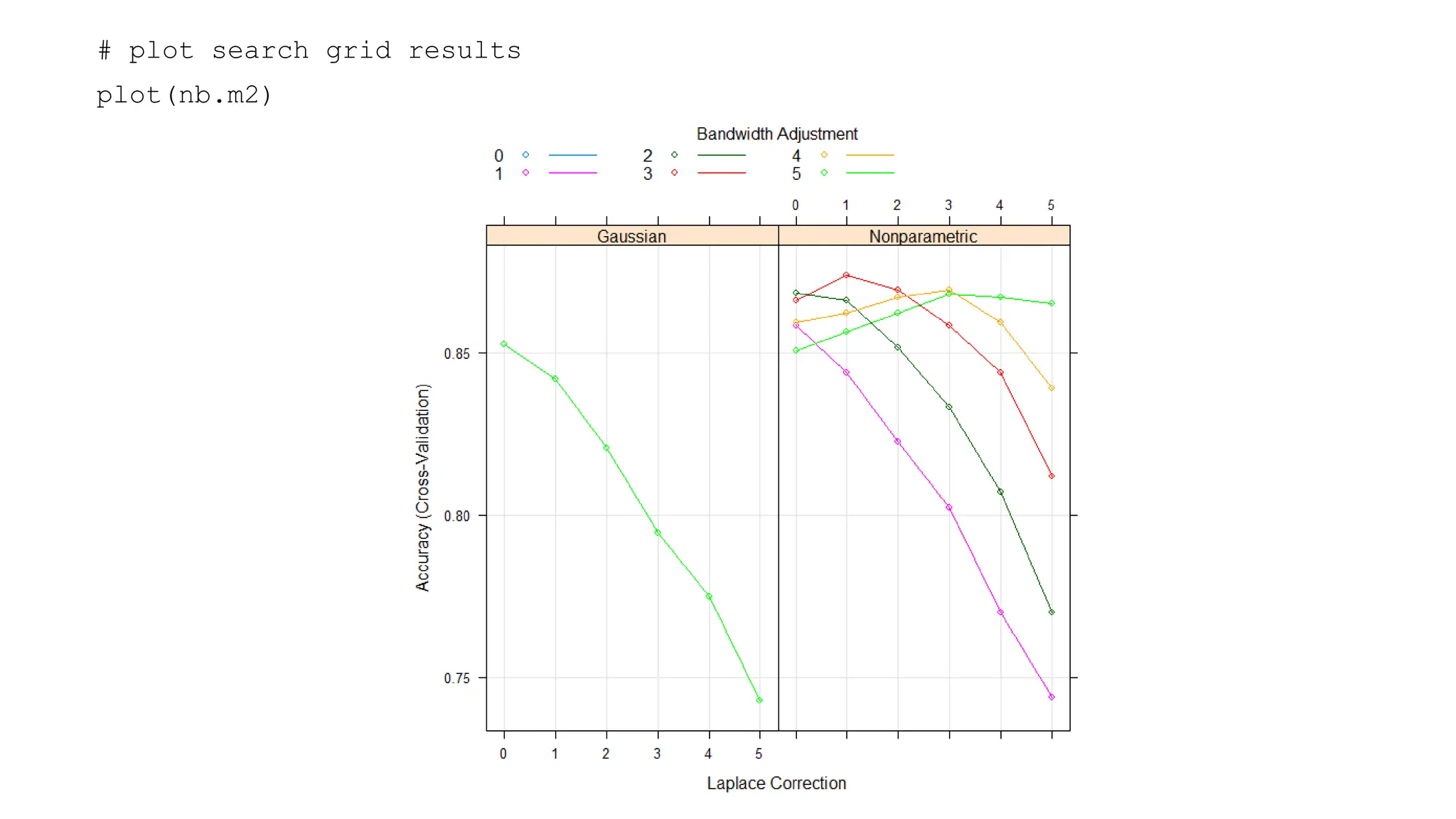
![# results for best model
confusionMatrix(nb.m2)
Cross-Validated (10 fold) Confusion Matrix
(entries are percentual average cell counts across resamples)
Reference
Prediction No Yes
No 81.2 9.9
Yes 2.7 6.2
Accuracy (average) : 0.8738
We can assess the accuracy on our final holdout test set.
pred <- predict(nb.m2, newdata = test)
confusionMatrix(pred, test$Attrition)
Confusion Matrix and Statistics
Reference
Prediction No Yes
No 349 41
Yes 20 30
Accuracy : 0.8614
95% CI : (0.8255, 0.8923)
No Information Rate : 0.8386
P-Value [Acc > NIR] : 0.10756
Kappa : 0.4183
Mcnemar's Test P-Value : 0.01045
Sensitivity : 0.9458
Specificity : 0.4225
Pos Pred Value : 0.8949
Neg Pred Value : 0.6000
Prevalence : 0.8386
Detection Rate : 0.7932
Detection Prevalence : 0.8864
Balanced Accuracy : 0.6842
'Positive' Class : No](https://image.slidesharecdn.com/naivebayesclassifier-250311155450-6f591eef/75/Naive-Bayes-Classifier-ppt-helping-others-by-sharing-the-ppt-37-2048.jpg)


![Naïve Bayes
• Bayes classification
Bayes classification
Difficulty: learning the joint probability
• Naïve Bayes classification
Naïve Bayes classification
– Assumption that all input attributes are conditionally
independent!
– MAP classification rule: for
)
(
)
|
,
,
(
)
(
)
(
)
( 1 C
P
C
X
X
P
C
P
C
|
P
|
C
P n
X
X
)
|
,
,
( 1 C
X
X
P n
)
|
(
)
|
(
)
|
(
)
|
,
,
(
)
|
(
)
|
,
,
(
)
,
,
,
|
(
)
|
,
,
,
(
2
1
2
1
2
2
1
2
1
C
X
P
C
X
P
C
X
P
C
X
X
P
C
X
P
C
X
X
P
C
X
X
X
P
C
X
X
X
P
n
n
n
n
n
L
n
n c
c
c
c
c
c
P
c
x
P
c
x
P
c
P
c
x
P
c
x
P ,
,
,
),
(
)]
|
(
)
|
(
[
)
(
)]
|
(
)
|
(
[ 1
*
1
*
*
*
1
)
,
,
,
( 2
1 n
x
x
x
x
For a class, the previous generative model can be
decomposed by n
n generative models of a single
input.
Product of
individual
probabilities](https://crownmelresort.com/image.slidesharecdn.com/naivebayesclassifier-250311155450-6f591eef/75/Naive-Bayes-Classifier-ppt-helping-others-by-sharing-the-ppt-10-2048.jpg)
![Naïve Bayes Algorithm
Naïve Bayes Algorithm
• Naïve Bayes Algorithm (for discrete input attributes) has two
phases
– 1. Learning Phase
1. Learning Phase: Given a training set S,
Output: conditional probability tables; for elements
– 2. Test Phase
2. Test Phase: Given an unknown instance ,
Look up tables to assign the label c* to X’ if
;
in
examples
with
)
|
(
estimate
)
|
(
ˆ
)
,
1
;
,
,
1
(
attribute
each
of
value
attribute
every
For
;
in
examples
with
)
(
estimate
)
(
ˆ
of
value
target
each
For 1
S
S
i
jk
j
i
jk
j
j
j
jk
i
i
L
i
i
c
C
x
X
P
c
C
x
X
P
N
,
k
n
j
X
x
c
C
P
c
C
P
)
c
,
,
c
(c
c
L
n
n c
c
c
c
c
c
P
c
a
P
c
a
P
c
P
c
a
P
c
a
P ,
,
,
),
(
ˆ
)]
|
(
ˆ
)
|
(
ˆ
[
)
(
ˆ
)]
|
(
ˆ
)
|
(
ˆ
[ 1
*
1
*
*
*
1
)
,
,
( 1 n
a
a
X
L
N
X j
j
,
Classification is easy, just multiply probabilities
Learning is easy, just
create probability tables.](https://crownmelresort.com/image.slidesharecdn.com/naivebayesclassifier-250311155450-6f591eef/75/Naive-Bayes-Classifier-ppt-helping-others-by-sharing-the-ppt-11-2048.jpg)


![The test phase
test phase for the tennis example
• Test Phase
– Given a new instance of variable values,
x’=(Outlook=Sunny, Temperature=Cool, Humidity=High, Wind=Strong)
– Given calculated Look up tables
– Use the
Use the MAP rule
MAP rule to calculate Yes or No
to calculate Yes or No
P(Outlook=Sunny|Play=No
No) = 3/5
P(Temperature=Cool|Play==No) = 1/5
P(Huminity=High|Play=No) = 4/5
P(Wind=Strong|Play=No) = 3/5
P(Play=No) = 5/14
P(Outlook=Sunny|Play=Yes
Yes) = 2/9
P(Temperature=Cool|Play=Yes) = 3/9
P(Huminity=High|Play=Yes) = 3/9
P(Wind=Strong|Play=Yes) = 3/9
P(Play=Yes) = 9/14
P(Yes|x’): [P(Sunny|Yes)P(Cool|Yes)P(High|Yes)P(Strong|Yes)]P(Play=Yes) = 0.0053
P(No|x’): [P(Sunny|No) P(Cool|No)P(High|No)P(Strong|No)]P(Play=No) = 0.0206
Given the fact P(
Given the fact P(Yes
Yes|
|x
x’) < P(
’) < P(No
No|
|x
x’), we label
’), we label x
x’ to be “
’ to be “No
No”.
”.](https://crownmelresort.com/image.slidesharecdn.com/naivebayesclassifier-250311155450-6f591eef/75/Naive-Bayes-Classifier-ppt-helping-others-by-sharing-the-ppt-15-2048.jpg)


![• First, we apply a naïve Bayes model with 10-fold cross validation, which gets 83%
accuracy. Considering about 83% of our observations in our training set do not attrit, our
overall accuracy is no better than if we just predicted “No” attrition for every observation.
• There are several packages to apply naïve Bayes (i.e. e1071, klaR, naivebayes, bnclassify).
library(klaR)
# create response and feature data
features <- setdiff(names(train), "Attrition")
x <- train[, features]
y <- train$Attrition
# set up 10-fold cross validation procedure
train_control <- trainControl(
method = "cv",
number = 10
)
# train model
nb.m1 <- train(
x = x,
y = y,
method = "nb",
trControl = train_control
)
# results
confusionMatrix(nb.m1)
Cross-Validated (10 fold) Confusion Matrix
(entries are percentual average cell counts across resamples)
Reference
Prediction No Yes
No 75.2 8.1
Yes 8.6 8.1
Accuracy (average) : 0.833](https://crownmelresort.com/image.slidesharecdn.com/naivebayesclassifier-250311155450-6f591eef/75/Naive-Bayes-Classifier-ppt-helping-others-by-sharing-the-ppt-33-2048.jpg)


![# results for best model
confusionMatrix(nb.m2)
Cross-Validated (10 fold) Confusion Matrix
(entries are percentual average cell counts across resamples)
Reference
Prediction No Yes
No 81.2 9.9
Yes 2.7 6.2
Accuracy (average) : 0.8738
We can assess the accuracy on our final holdout test set.
pred <- predict(nb.m2, newdata = test)
confusionMatrix(pred, test$Attrition)
Confusion Matrix and Statistics
Reference
Prediction No Yes
No 349 41
Yes 20 30
Accuracy : 0.8614
95% CI : (0.8255, 0.8923)
No Information Rate : 0.8386
P-Value [Acc > NIR] : 0.10756
Kappa : 0.4183
Mcnemar's Test P-Value : 0.01045
Sensitivity : 0.9458
Specificity : 0.4225
Pos Pred Value : 0.8949
Neg Pred Value : 0.6000
Prevalence : 0.8386
Detection Rate : 0.7932
Detection Prevalence : 0.8864
Balanced Accuracy : 0.6842
'Positive' Class : No](https://crownmelresort.com/image.slidesharecdn.com/naivebayesclassifier-250311155450-6f591eef/75/Naive-Bayes-Classifier-ppt-helping-others-by-sharing-the-ppt-37-2048.jpg)


