This document discusses Naive Bayes classifiers. It begins with an overview of probabilistic classification and the Naive Bayes approach. The Naive Bayes classifier makes a strong independence assumption that features are conditionally independent given the class. It then presents the algorithm for Naive Bayes classification with discrete and continuous features. An example of classifying whether to play tennis is used to illustrate the learning and classification phases. The document concludes with a discussion of some relevant issues and a high-level summary of Naive Bayes.
Introduction to Naïve Bayes Classifier in Machine Learning by Ke Chen, including background and outline of presentation topics.
Classification methods categorized: direct rule modeling (k-NN, Decision Trees) and probabilistic models (naïve Bayes), highlighting discriminative vs generative classification.
Basic concepts of probability including prior, conditional, joint probabilities and Bayes' rule, supplemented by a quiz on probabilities with dice.
Establishing probabilistic classification models using both discriminative and generative approaches, and defining MAP classification rule.
Overview of Naïve Bayes classification, focusing on the independence assumption and algorithm for discrete-valued features in learning and testing phases.
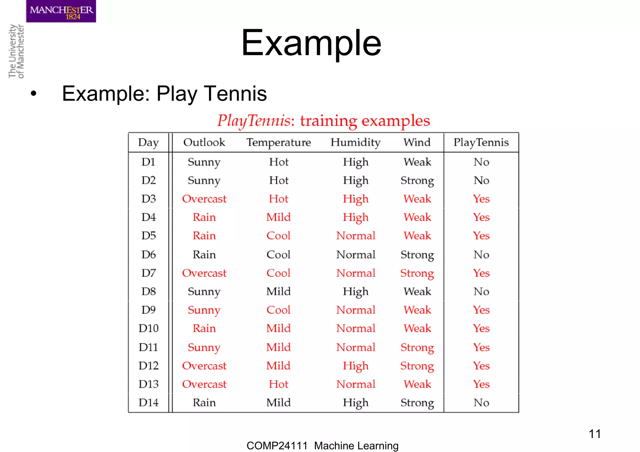
Example of applying Naïve Bayes using a dataset on playing tennis, detailing learning and testing phases, showcasing probability computations.
Application of Naïve Bayes to continuous-valued features using normal distribution for calculations in training and testing phases.
Addressing the issues of independence assumption violations and zero conditional probability in Naïve Bayes, emphasizing its effectiveness and applications.
COMP24111 Machine Learning
2
Outline
•Background
• Probability Basics
• Probabilistic Classification
• Naïve Bayes
– Principle and Algorithms
– Example: Play Tennis
• Relevant Issues
• Summary
3.
COMP24111 Machine Learning
3
Background
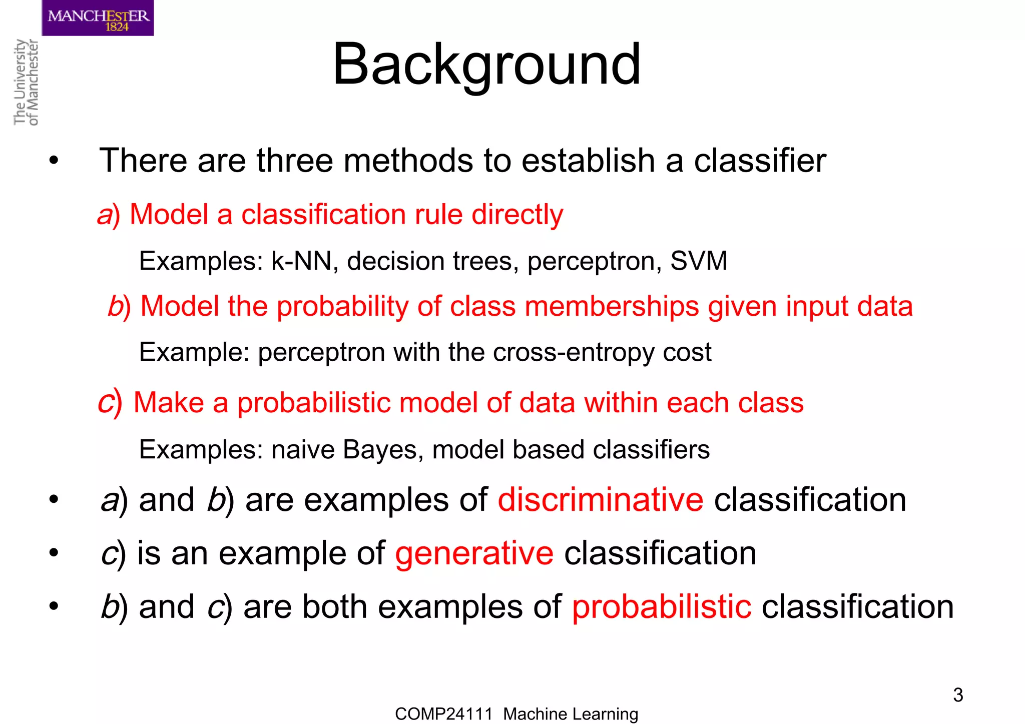
•There are three methods to establish a classifier
a) Model a classification rule directly
Examples: k-NN, decision trees, perceptron, SVM
b) Model the probability of class memberships given input data
Example: perceptron with the cross-entropy cost
c) Make a probabilistic model of data within each class
Examples: naive Bayes, model based classifiers
• a) and b) are examples of discriminative classification
• c) is an example of generative classification
• b) and c) are both examples of probabilistic classification
4.
COMP24111 Machine Learning
4
ProbabilityBasics
• Prior, conditional and joint probability for random variables
– Prior probability:
– Conditional probability:
– Joint probability:
– Relationship:
– Independence:
• Bayesian Rule
)|,)( 121 XP(XX|XP 2
)(
)()(
)(
X
X
X
P
CPC|P
|CP =
)(XP
))(),,( 22 ,XP(XPXX 11 == XX
)()|()()|() 2211122 XPXXPXPXXP,XP(X1 ==
)()()),()|(),()|( 212121212 XPXP,XP(XXPXXPXPXXP 1 ===
Evidence
PriorLikelihood
Posterior
×
=
5.
COMP24111 Machine Learning
5
ProbabilityBasics
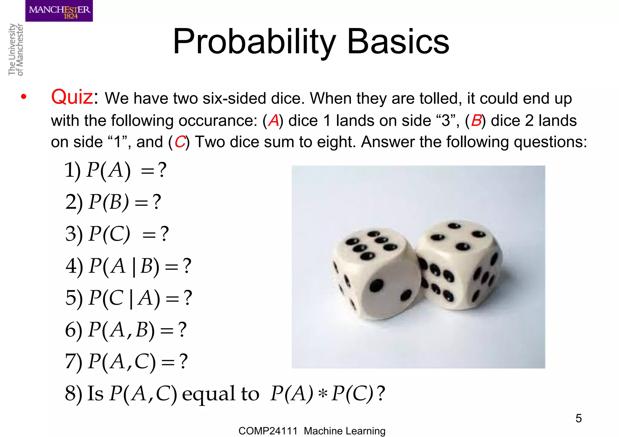
• Quiz: We have two six-sided dice. When they are tolled, it could end up
with the following occurance: (A) dice 1 lands on side “3”, (B) dice 2 lands
on side “1”, and (C) Two dice sum to eight. Answer the following questions:
?toequal),(Is8)
?),(7)
?),(6)
?)|(5)
?)|(4)
?3)
?2)
?)()1
P(C)P(A)CAP
CAP
BAP
ACP
BAP
P(C)
P(B)
AP
∗
=
=
=
=
=
=
=
6.
COMP24111 Machine Learning
6
ProbabilisticClassification
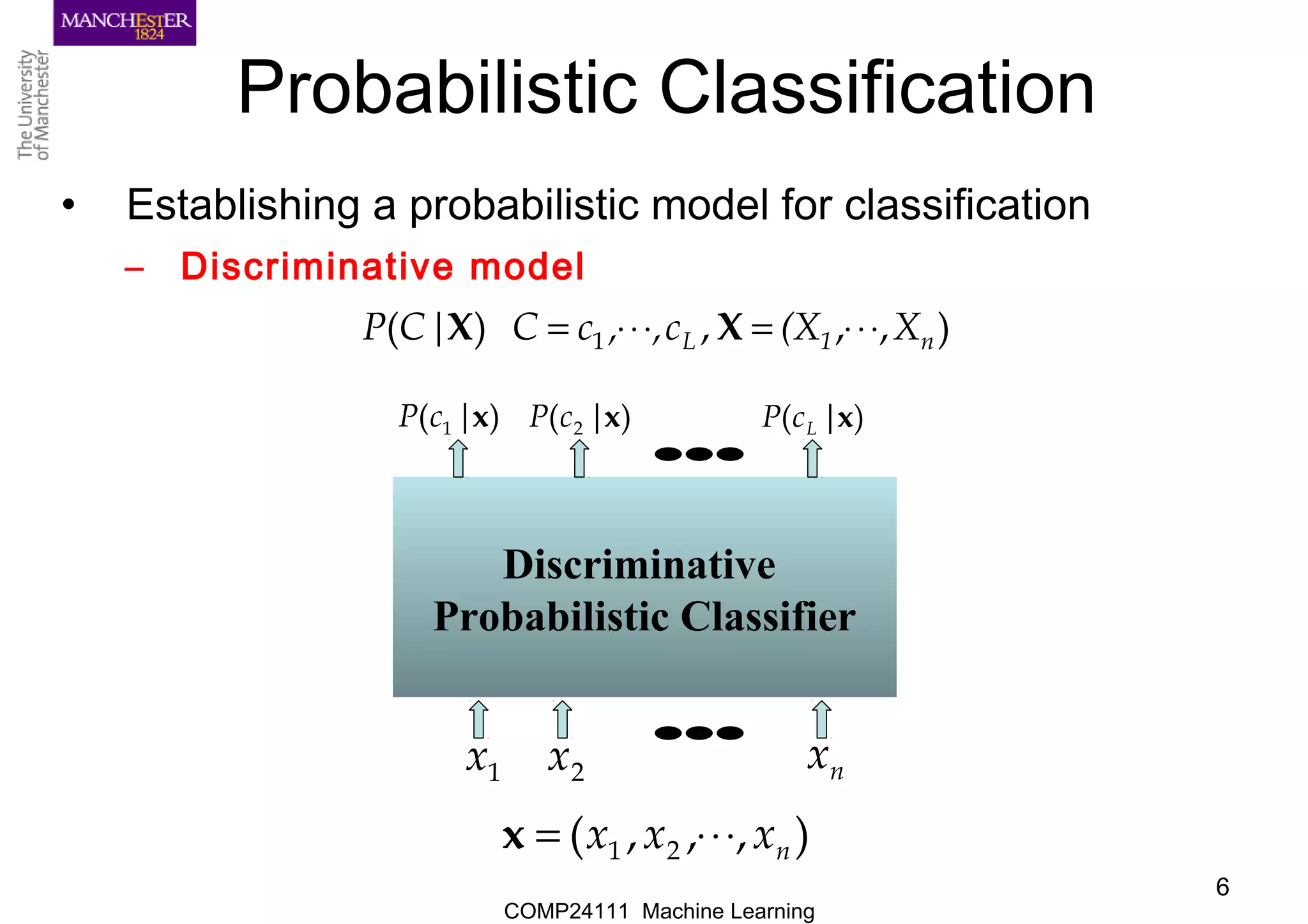
• Establishing a probabilistic model for classification
– Discriminative model
),,,)( 1 n1L X(Xc,,cC|CP ⋅⋅⋅=⋅⋅⋅= XX
),,,( 21 nxxx ⋅⋅⋅=x
Discriminative
Probabilistic Classifier
1x 2x nx
)|( 1 xcP )|( 2 xcP )|( xLcP
•••
•••
7.
COMP24111 Machine Learning
7
ProbabilisticClassification
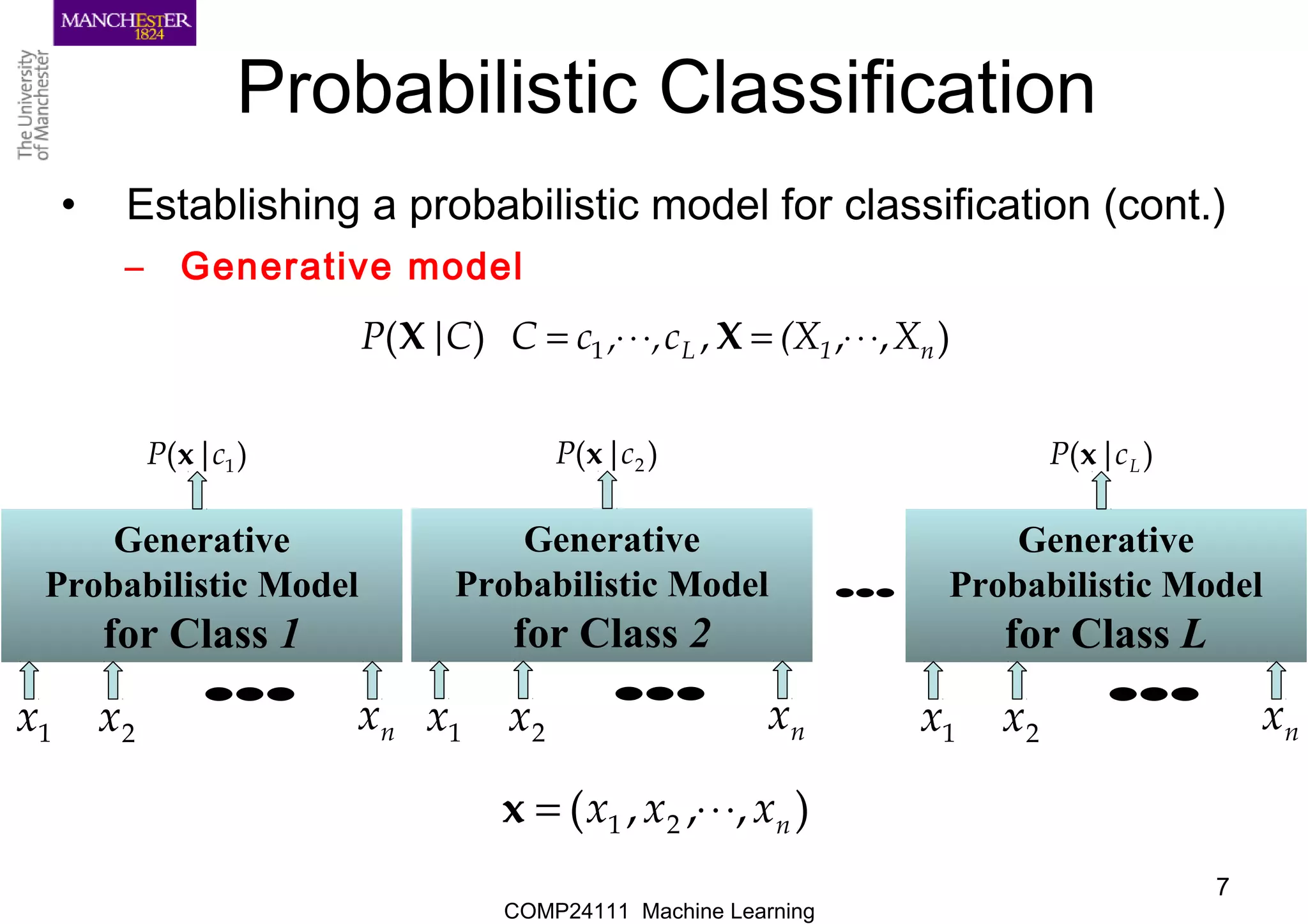
• Establishing a probabilistic model for classification (cont.)
– Generative model
),,,)( 1 n1L X(Xc,,cCC|P ⋅⋅⋅=⋅⋅⋅= XX
Generative
Probabilistic Model
for Class 1
)|( 1cP x
1x 2x nx
•••
Generative
Probabilistic Model
for Class 2
)|( 2cP x
1x 2x nx
•••
Generative
Probabilistic Model
for Class L
)|( LcP x
1x 2x nx
•••
•••
),,,( 21 nxxx ⋅⋅⋅=x
8.
COMP24111 Machine Learning
8
ProbabilisticClassification
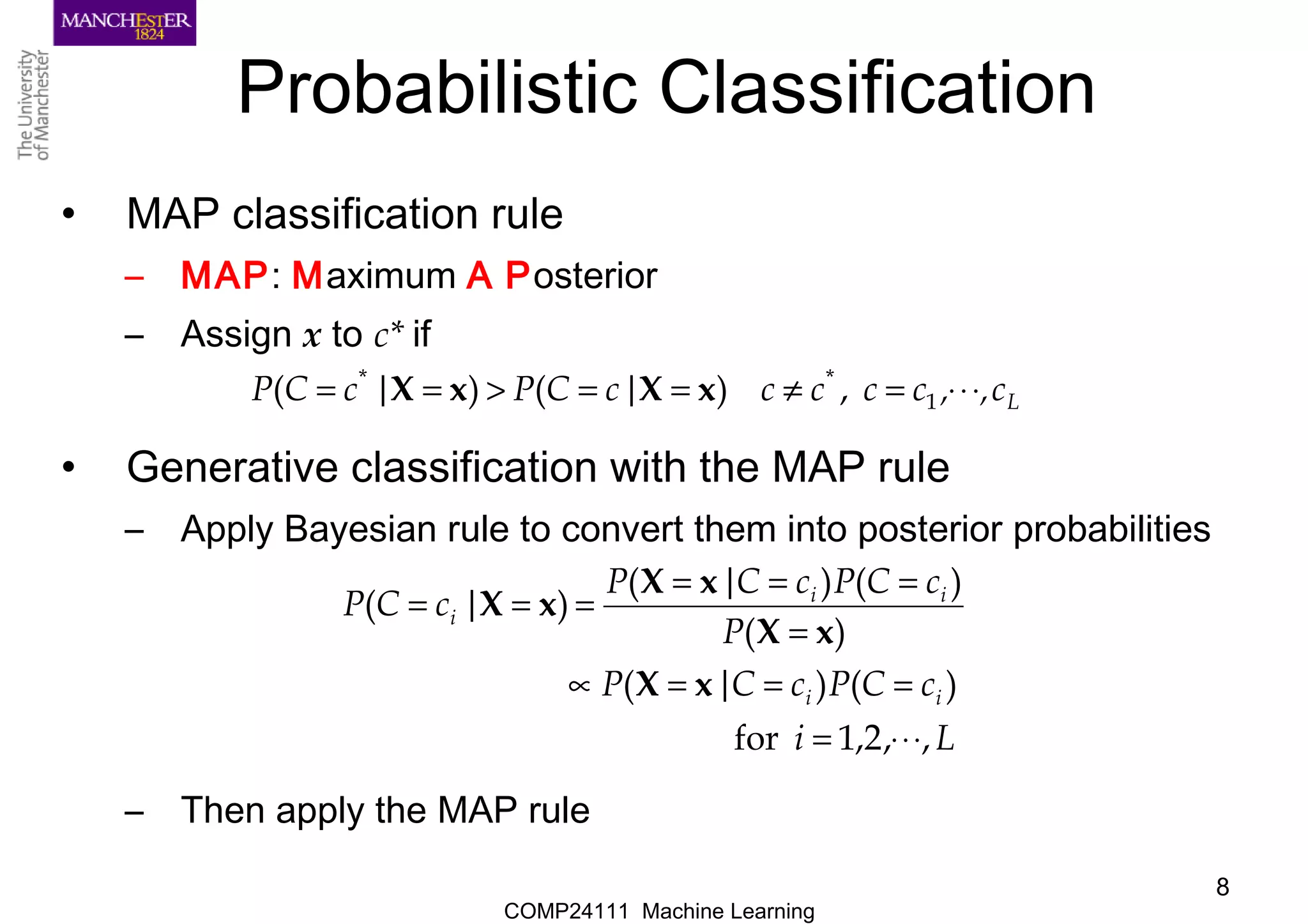
• MAP classification rule
– MAP: Maximum A Posterior
– Assign x to c* if
• Generative classification with the MAP rule
– Apply Bayesian rule to convert them into posterior probabilities
– Then apply the MAP rule
Lc,,cccc|cCP|cCP ⋅⋅⋅=≠==>== 1
**
,)()( xXxX
Li
cCPcC|P
P
cCPcC|P
|cCP
ii
ii
i
,,2,1for
)()(
)(
)()(
)(
⋅⋅⋅=
===∝
=
===
===
xX
xX
xX
xX
9.
COMP24111 Machine Learning
9
NaïveBayes
• Bayes classification
Difficulty: learning the joint probability
• Naïve Bayes classification
– Assumption that all input features are conditionally independent!
– MAP classification rule: for
)()|,,()()()( 1 CPCXXPCPC|P|CP n⋅⋅⋅=∝ XX
)|,,( 1 CXXP n⋅⋅⋅
)|()|()|(
)|,,()|(
)|,,(),,,|()|,,,(
21
21
22121
CXPCXPCXP
CXXPCXP
CXXPCXXXPCXXXP
n
n
nnn
⋅⋅⋅=
⋅⋅⋅=
⋅⋅⋅⋅⋅⋅=⋅⋅⋅
Lnn ccccccPcxPcxPcPcxPcxP ,,,),()]|()|([)()]|()|([ 1
*
1
***
1 ⋅⋅⋅=≠⋅⋅⋅>⋅⋅⋅
),,,( 21 nxxx ⋅⋅⋅=x
10.
COMP24111 Machine Learning
10
NaïveBayes
• Algorithm: Discrete-Valued Features
– Learning Phase: Given a training set S,
Output: conditional probability tables; for elements
– Test Phase: Given an unknown instance ,
Look up tables to assign the label c* to X’ if
;inexampleswith)|(estimate)|(ˆ
),1;,,1(featureeachofvaluefeatureeveryFor
;inexampleswith)(estimate)(ˆ
ofvaluetargeteachFor 1
S
S
ijkjijkj
jjjk
ii
Lii
cCxXPcCxXP
N,knjXx
cCPcCP
)c,,c(cc
==←==
⋅⋅⋅=⋅⋅⋅=
=←=
⋅⋅⋅=
Lnn ccccccPcaPcaPcPcaPcaP ,,,),(ˆ)]|(ˆ)|(ˆ[)(ˆ)]|(ˆ)|(ˆ[ 1
*
1
***
1 ⋅⋅⋅=≠′⋅⋅⋅′>′⋅⋅⋅′
),,( 1 naa ′⋅⋅⋅′=′X
LNX jj ×,
COMP24111 Machine Learning
12
Example
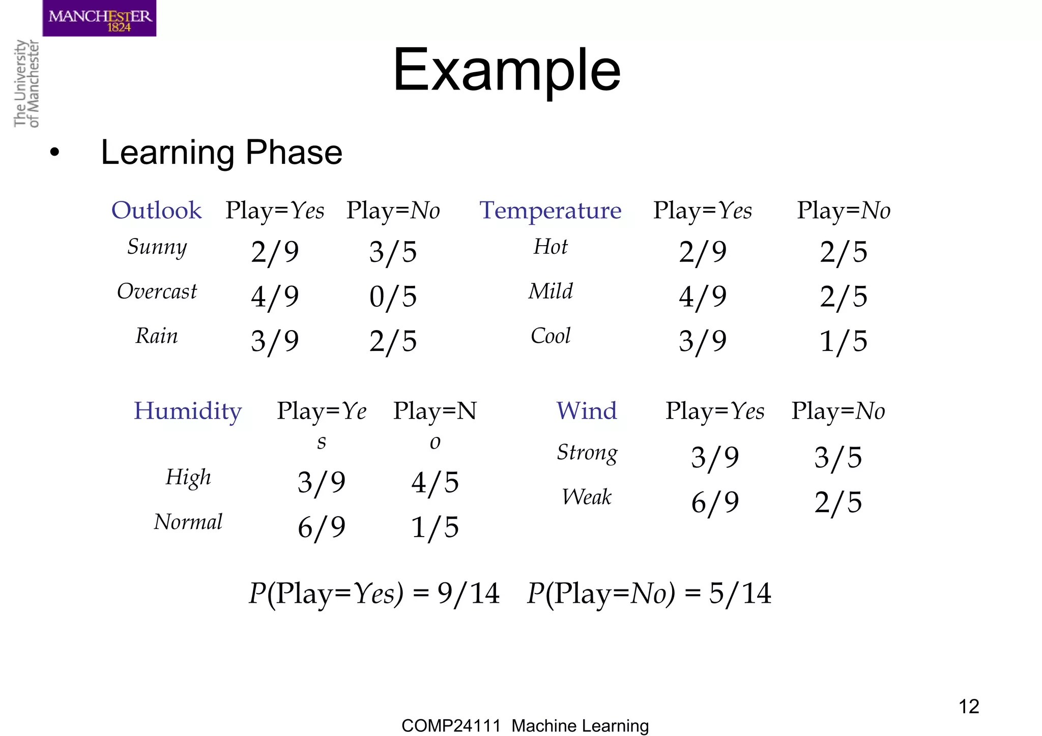
•Learning Phase
Outlook Play=Yes Play=No
Sunny 2/9 3/5
Overcast 4/9 0/5
Rain 3/9 2/5
Temperature Play=Yes Play=No
Hot 2/9 2/5
Mild 4/9 2/5
Cool 3/9 1/5
Humidity Play=Ye
s
Play=N
o
High 3/9 4/5
Normal 6/9 1/5
Wind Play=Yes Play=No
Strong 3/9 3/5
Weak 6/9 2/5
P(Play=Yes) = 9/14 P(Play=No) = 5/14
13.
COMP24111 Machine Learning
13
Example
•Test Phase
– Given a new instance, predict its label
x’=(Outlook=Sunny, Temperature=Cool, Humidity=High, Wind=Strong)
– Look up tables achieved in the learning phrase
– Decision making with the MAP rule
P(Outlook=Sunny|Play=No) = 3/5
P(Temperature=Cool|Play==No) = 1/5
P(Huminity=High|Play=No) = 4/5
P(Wind=Strong|Play=No) = 3/5
P(Play=No) = 5/14
P(Outlook=Sunny|Play=Yes) = 2/9
P(Temperature=Cool|Play=Yes) = 3/9
P(Huminity=High|Play=Yes) = 3/9
P(Wind=Strong|Play=Yes) = 3/9
P(Play=Yes) = 9/14
P(Yes|x’): [P(Sunny|Yes)P(Cool|Yes)P(High|Yes)P(Strong|Yes)]P(Play=Yes) =
0.0053
P(No|x’): [P(Sunny|No) P(Cool|No)P(High|No)P(Strong|No)]P(Play=No) = 0.0206
Given the fact P(Yes|x’) < P(No|x’), we label x’ to be “No”.
14.
COMP24111 Machine Learning
14
Example
•Test Phase
– Given a new instance,
x’=(Outlook=Sunny, Temperature=Cool, Humidity=High, Wind=Strong)
– Look up tables
– MAP rule
P(Outlook=Sunny|Play=No) = 3/5
P(Temperature=Cool|Play==No) = 1/5
P(Huminity=High|Play=No) = 4/5
P(Wind=Strong|Play=No) = 3/5
P(Play=No) = 5/14
P(Outlook=Sunny|Play=Yes) = 2/9
P(Temperature=Cool|Play=Yes) = 3/9
P(Huminity=High|Play=Yes) = 3/9
P(Wind=Strong|Play=Yes) = 3/9
P(Play=Yes) = 9/14
P(Yes|x’): [P(Sunny|Yes)P(Cool|Yes)P(High|Yes)P(Strong|Yes)]P(Play=Yes) =
0.0053
P(No|x’): [P(Sunny|No) P(Cool|No)P(High|No)P(Strong|No)]P(Play=No) = 0.0206
Given the fact P(Yes|x’) < P(No|x’), we label x’ to be “No”.
15.
COMP24111 Machine Learning
15
NaïveBayes
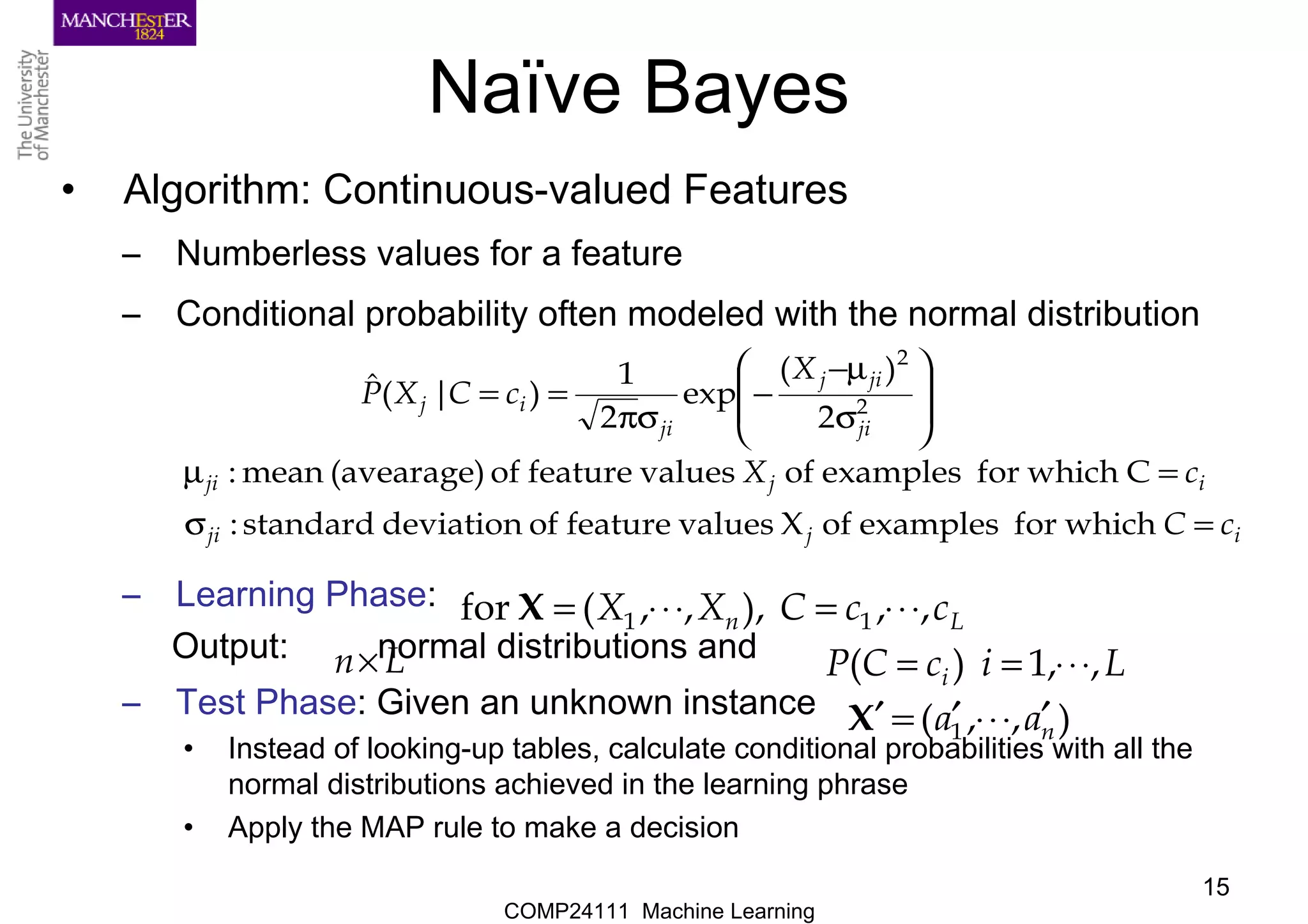
• Algorithm: Continuous-valued Features
– Numberless values for a feature
– Conditional probability often modeled with the normal distribution
– Learning Phase:
Output: normal distributions and
– Test Phase: Given an unknown instance
• Instead of looking-up tables, calculate conditional probabilities with all the
normal distributions achieved in the learning phrase
• Apply the MAP rule to make a decision
ijji
ijji
ji
jij
ji
ij
cC
cX
X
cCXP
=σ
=µ
σ
µ−
−
σπ
==
whichforexamplesofXvaluesfeatureofdeviationstandard:
Cwhichforexamplesofvaluesfeatureof(avearage)mean:
2
)(
exp
2
1
)|(ˆ
2
2
Ln ccCXX ,,),,,(for 11 ⋅⋅⋅=⋅⋅⋅=X
Ln× LicCP i ,,1)( ⋅⋅⋅==
),,( 1 naa ′⋅⋅⋅′=′X
16.
COMP24111 Machine Learning
16
NaïveBayes
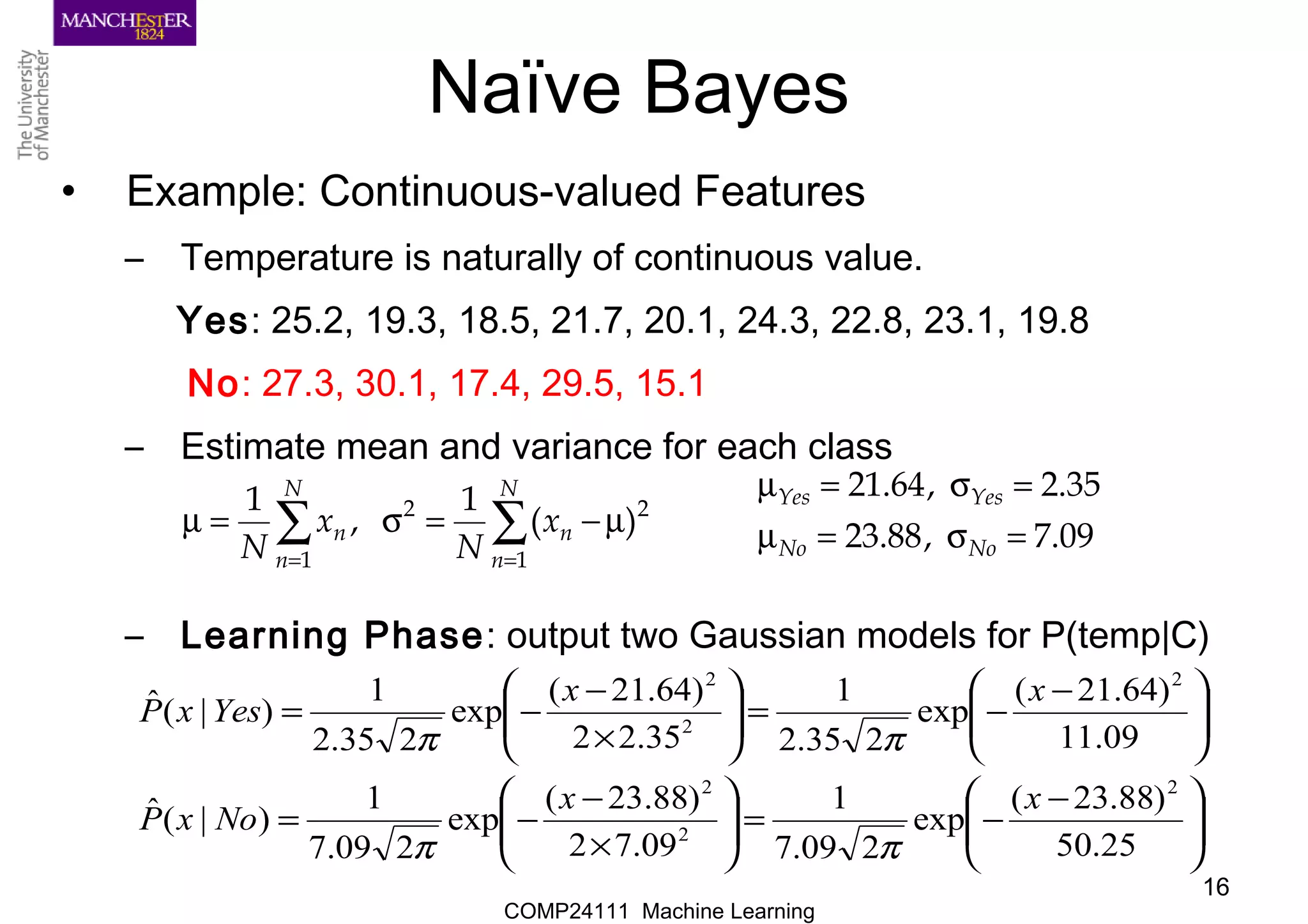
• Example: Continuous-valued Features
– Temperature is naturally of continuous value.
Yes: 25.2, 19.3, 18.5, 21.7, 20.1, 24.3, 22.8, 23.1, 19.8
No: 27.3, 30.1, 17.4, 29.5, 15.1
– Estimate mean and variance for each class
– Learning Phase: output two Gaussian models for P(temp|C)
∑∑
==
µ−=σ=µ
N
n
n
N
n
n x
N
x
N 1
22
1
)(
1
,
1
09.7,88.23
35.2,64.21
=σ=µ
=σ=µ
NoNo
YesYes
−
−=
×
−
−=
−
−=
×
−
−=
25.50
)88.23(
exp
209.7
1
09.72
)88.23(
exp
209.7
1
)|(ˆ
09.11
)64.21(
exp
235.2
1
35.22
)64.21(
exp
235.2
1
)|(ˆ
2
2
2
2
2
2
xx
NoxP
xx
YesxP
ππ
ππ
17.
COMP24111 Machine Learning
17
RelevantIssues
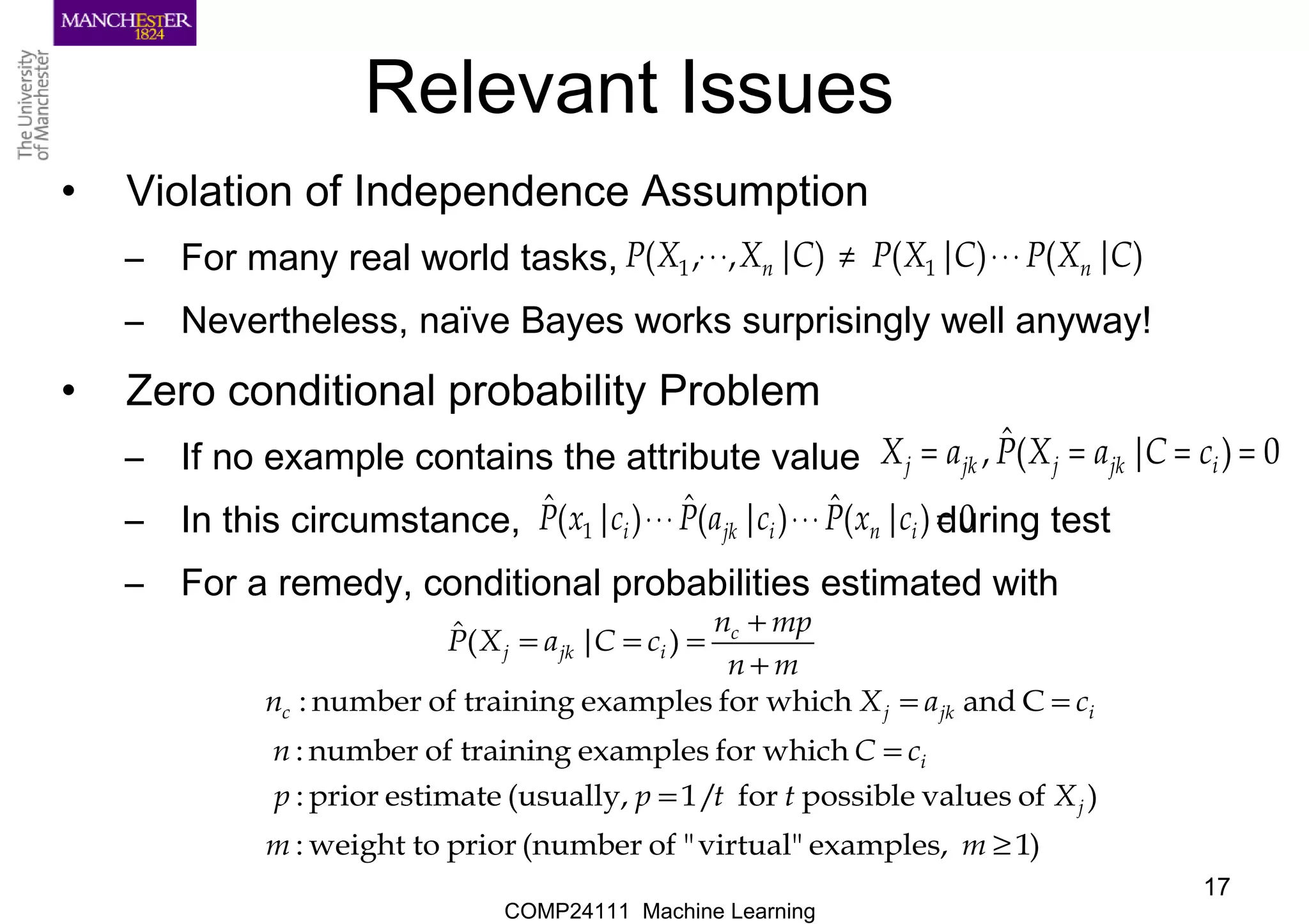
• Violation of Independence Assumption
– For many real world tasks,
– Nevertheless, naïve Bayes works surprisingly well anyway!
• Zero conditional probability Problem
– If no example contains the attribute value
– In this circumstance, during test
– For a remedy, conditional probabilities estimated with
)|()|()|,,( 11 CXPCXPCXXP nn ⋅⋅⋅≠⋅⋅⋅
0)|(ˆ, ==== ijkjjkj cCaXPaX
0)|(ˆ)|(ˆ)|(ˆ
1 =⋅⋅⋅⋅⋅⋅ inijki cxPcaPcxP
)1examples,virtual""of(numberpriortoweight:
)ofvaluespossiblefor/1(usually,estimateprior:
whichforexamplestrainingofnumber:
Candwhichforexamplestrainingofnumber:
)|(ˆ
≥
=
=
==
+
+
===
mm
Xttpp
cCn
caXn
mn
mpn
cCaXP
j
i
ijkjc
c
ijkj
18.
COMP24111 Machine Learning
18
Summary
•Naïve Bayes: the conditional independence assumption
– Training is very easy and fast; just requiring considering each
attribute in each class separately
– Test is straightforward; just looking up tables or calculating
conditional probabilities with estimated distributions
• A popular generative model
– Performance competitive to most of state-of-the-art classifiers
even in presence of violating independence assumption
– Many successful applications, e.g., spam mail filtering
– A good candidate of a base learner in ensemble learning
– Apart from classification, naïve Bayes can do more…
Editor's Notes
#10 For a class, the previous generative model can be decomposed by n generative models of a single input.


![COMP24111 Machine Learning
9
Naïve Bayes
• Bayes classification
Difficulty: learning the joint probability
• Naïve Bayes classification
– Assumption that all input features are conditionally independent!
– MAP classification rule: for
)()|,,()()()( 1 CPCXXPCPC|P|CP n⋅⋅⋅=∝ XX
)|,,( 1 CXXP n⋅⋅⋅
)|()|()|(
)|,,()|(
)|,,(),,,|()|,,,(
21
21
22121
CXPCXPCXP
CXXPCXP
CXXPCXXXPCXXXP
n
n
nnn
⋅⋅⋅=
⋅⋅⋅=
⋅⋅⋅⋅⋅⋅=⋅⋅⋅
Lnn ccccccPcxPcxPcPcxPcxP ,,,),()]|()|([)()]|()|([ 1
*
1
***
1 ⋅⋅⋅=≠⋅⋅⋅>⋅⋅⋅
),,,( 21 nxxx ⋅⋅⋅=x](https://image.slidesharecdn.com/naive-bayes-150514165844-lva1-app6891/75/Naive-bayes-9-2048.jpg)
![COMP24111 Machine Learning
10
Naïve Bayes
• Algorithm: Discrete-Valued Features
– Learning Phase: Given a training set S,
Output: conditional probability tables; for elements
– Test Phase: Given an unknown instance ,
Look up tables to assign the label c* to X’ if
;inexampleswith)|(estimate)|(ˆ
),1;,,1(featureeachofvaluefeatureeveryFor
;inexampleswith)(estimate)(ˆ
ofvaluetargeteachFor 1
S
S
ijkjijkj
jjjk
ii
Lii
cCxXPcCxXP
N,knjXx
cCPcCP
)c,,c(cc
==←==
⋅⋅⋅=⋅⋅⋅=
=←=
⋅⋅⋅=
Lnn ccccccPcaPcaPcPcaPcaP ,,,),(ˆ)]|(ˆ)|(ˆ[)(ˆ)]|(ˆ)|(ˆ[ 1
*
1
***
1 ⋅⋅⋅=≠′⋅⋅⋅′>′⋅⋅⋅′
),,( 1 naa ′⋅⋅⋅′=′X
LNX jj ×,](https://image.slidesharecdn.com/naive-bayes-150514165844-lva1-app6891/75/Naive-bayes-10-2048.jpg)
![COMP24111 Machine Learning
13
Example
• Test Phase
– Given a new instance, predict its label
x’=(Outlook=Sunny, Temperature=Cool, Humidity=High, Wind=Strong)
– Look up tables achieved in the learning phrase
– Decision making with the MAP rule
P(Outlook=Sunny|Play=No) = 3/5
P(Temperature=Cool|Play==No) = 1/5
P(Huminity=High|Play=No) = 4/5
P(Wind=Strong|Play=No) = 3/5
P(Play=No) = 5/14
P(Outlook=Sunny|Play=Yes) = 2/9
P(Temperature=Cool|Play=Yes) = 3/9
P(Huminity=High|Play=Yes) = 3/9
P(Wind=Strong|Play=Yes) = 3/9
P(Play=Yes) = 9/14
P(Yes|x’): [P(Sunny|Yes)P(Cool|Yes)P(High|Yes)P(Strong|Yes)]P(Play=Yes) =
0.0053
P(No|x’): [P(Sunny|No) P(Cool|No)P(High|No)P(Strong|No)]P(Play=No) = 0.0206
Given the fact P(Yes|x’) < P(No|x’), we label x’ to be “No”.](https://image.slidesharecdn.com/naive-bayes-150514165844-lva1-app6891/75/Naive-bayes-13-2048.jpg)
![COMP24111 Machine Learning
14
Example
• Test Phase
– Given a new instance,
x’=(Outlook=Sunny, Temperature=Cool, Humidity=High, Wind=Strong)
– Look up tables
– MAP rule
P(Outlook=Sunny|Play=No) = 3/5
P(Temperature=Cool|Play==No) = 1/5
P(Huminity=High|Play=No) = 4/5
P(Wind=Strong|Play=No) = 3/5
P(Play=No) = 5/14
P(Outlook=Sunny|Play=Yes) = 2/9
P(Temperature=Cool|Play=Yes) = 3/9
P(Huminity=High|Play=Yes) = 3/9
P(Wind=Strong|Play=Yes) = 3/9
P(Play=Yes) = 9/14
P(Yes|x’): [P(Sunny|Yes)P(Cool|Yes)P(High|Yes)P(Strong|Yes)]P(Play=Yes) =
0.0053
P(No|x’): [P(Sunny|No) P(Cool|No)P(High|No)P(Strong|No)]P(Play=No) = 0.0206
Given the fact P(Yes|x’) < P(No|x’), we label x’ to be “No”.](https://image.slidesharecdn.com/naive-bayes-150514165844-lva1-app6891/75/Naive-bayes-14-2048.jpg)


![COMP24111 Machine Learning
9
Naïve Bayes
• Bayes classification
Difficulty: learning the joint probability
• Naïve Bayes classification
– Assumption that all input features are conditionally independent!
– MAP classification rule: for
)()|,,()()()( 1 CPCXXPCPC|P|CP n⋅⋅⋅=∝ XX
)|,,( 1 CXXP n⋅⋅⋅
)|()|()|(
)|,,()|(
)|,,(),,,|()|,,,(
21
21
22121
CXPCXPCXP
CXXPCXP
CXXPCXXXPCXXXP
n
n
nnn
⋅⋅⋅=
⋅⋅⋅=
⋅⋅⋅⋅⋅⋅=⋅⋅⋅
Lnn ccccccPcxPcxPcPcxPcxP ,,,),()]|()|([)()]|()|([ 1
*
1
***
1 ⋅⋅⋅=≠⋅⋅⋅>⋅⋅⋅
),,,( 21 nxxx ⋅⋅⋅=x](https://crownmelresort.com/image.slidesharecdn.com/naive-bayes-150514165844-lva1-app6891/75/Naive-bayes-9-2048.jpg)
![COMP24111 Machine Learning
10
Naïve Bayes
• Algorithm: Discrete-Valued Features
– Learning Phase: Given a training set S,
Output: conditional probability tables; for elements
– Test Phase: Given an unknown instance ,
Look up tables to assign the label c* to X’ if
;inexampleswith)|(estimate)|(ˆ
),1;,,1(featureeachofvaluefeatureeveryFor
;inexampleswith)(estimate)(ˆ
ofvaluetargeteachFor 1
S
S
ijkjijkj
jjjk
ii
Lii
cCxXPcCxXP
N,knjXx
cCPcCP
)c,,c(cc
==←==
⋅⋅⋅=⋅⋅⋅=
=←=
⋅⋅⋅=
Lnn ccccccPcaPcaPcPcaPcaP ,,,),(ˆ)]|(ˆ)|(ˆ[)(ˆ)]|(ˆ)|(ˆ[ 1
*
1
***
1 ⋅⋅⋅=≠′⋅⋅⋅′>′⋅⋅⋅′
),,( 1 naa ′⋅⋅⋅′=′X
LNX jj ×,](https://crownmelresort.com/image.slidesharecdn.com/naive-bayes-150514165844-lva1-app6891/75/Naive-bayes-10-2048.jpg)


![COMP24111 Machine Learning
13
Example
• Test Phase
– Given a new instance, predict its label
x’=(Outlook=Sunny, Temperature=Cool, Humidity=High, Wind=Strong)
– Look up tables achieved in the learning phrase
– Decision making with the MAP rule
P(Outlook=Sunny|Play=No) = 3/5
P(Temperature=Cool|Play==No) = 1/5
P(Huminity=High|Play=No) = 4/5
P(Wind=Strong|Play=No) = 3/5
P(Play=No) = 5/14
P(Outlook=Sunny|Play=Yes) = 2/9
P(Temperature=Cool|Play=Yes) = 3/9
P(Huminity=High|Play=Yes) = 3/9
P(Wind=Strong|Play=Yes) = 3/9
P(Play=Yes) = 9/14
P(Yes|x’): [P(Sunny|Yes)P(Cool|Yes)P(High|Yes)P(Strong|Yes)]P(Play=Yes) =
0.0053
P(No|x’): [P(Sunny|No) P(Cool|No)P(High|No)P(Strong|No)]P(Play=No) = 0.0206
Given the fact P(Yes|x’) < P(No|x’), we label x’ to be “No”.](https://crownmelresort.com/image.slidesharecdn.com/naive-bayes-150514165844-lva1-app6891/75/Naive-bayes-13-2048.jpg)
![COMP24111 Machine Learning
14
Example
• Test Phase
– Given a new instance,
x’=(Outlook=Sunny, Temperature=Cool, Humidity=High, Wind=Strong)
– Look up tables
– MAP rule
P(Outlook=Sunny|Play=No) = 3/5
P(Temperature=Cool|Play==No) = 1/5
P(Huminity=High|Play=No) = 4/5
P(Wind=Strong|Play=No) = 3/5
P(Play=No) = 5/14
P(Outlook=Sunny|Play=Yes) = 2/9
P(Temperature=Cool|Play=Yes) = 3/9
P(Huminity=High|Play=Yes) = 3/9
P(Wind=Strong|Play=Yes) = 3/9
P(Play=Yes) = 9/14
P(Yes|x’): [P(Sunny|Yes)P(Cool|Yes)P(High|Yes)P(Strong|Yes)]P(Play=Yes) =
0.0053
P(No|x’): [P(Sunny|No) P(Cool|No)P(High|No)P(Strong|No)]P(Play=No) = 0.0206
Given the fact P(Yes|x’) < P(No|x’), we label x’ to be “No”.](https://crownmelresort.com/image.slidesharecdn.com/naive-bayes-150514165844-lva1-app6891/75/Naive-bayes-14-2048.jpg)


![[Redis Released]- FalkorDB - Redis + Graph Agentic Memory’s Secret Sauce](https://cdn.slidesharecdn.com/ss_thumbnails/redisreleased-falkordbslidedeck-1125-251115194922-e1c0046b-thumbnail.jpg?width=640&height=640&fit=bounds)


