MATH 4513 NumericalAnalysis
Chapter 2. Solutions of Equations in One Variable
Xu Zhang
Assistant Professor
Department of Mathematics
Oklahoma State University
Text Book: Numerical Analysis (10th edition)
R. L. Burden, D. J. Faires, A. M. Burden
Xu Zhang (Oklahoma State University) MATH 4513 Numerical Analysis Fall 2020 1 / 70
2.
Chapter 2. Solutionsof Equations in One Variable
Chapter 2. Solutions of Equations in One Variable
Contents
2.1 The Bisection Method
2.2 Fixed-Point Iteration
2.3 Newton’s Method and Its Extensions
2.4 Error Analysis for Iterative Methods
Xu Zhang (Oklahoma State University) MATH 4513 Numerical Analysis Fall 2020 2 / 70
3.
Chapter 2. Solutionsof Equations in One Variable 2.1 The Bisection Method
Section 2.1 The Bisection Method
Starting from this section, we study the most basic mathematics
problem: root-finding problem
f(x) = 0.
The first numerical method, based on the Intermediate Value
Theorem (IVT), is called the Bisection Method.
Suppose that f(x) is continuous on [a, b]. f(a) and f(b) have
opposite sign. By IVT, there exists a number p ∈ (a, b) such that
f(p) = 0. That is, f(x) has a root in (a, b).
Idea of Bisection Method: repeatedly halve the subinterval of
[a, b], and at each step, locating the half containing the root.
Xu Zhang (Oklahoma State University) MATH 4513 Numerical Analysis Fall 2020 3 / 70
4.
Chapter 2. Solutionsof Equations in One Variable 2.1 The Bisection Method
Set a1 ← a, b1 ← b. Calculate the midpoint p1 ← a1+b1
2 .
2.1 The Bisection Method 49
Figure 2.1
x
y
f(a)
f(p2)
f (p1)
f(b)
y f(x)
a a1 b b1
p p1
p2
p3
a1 b1
p1
p2
a2 b2
p3
a3 b3
ALGORITHM
2.1
Bisection
To find a solution to f (x) = 0 given the continuous function f on the interval [a, b], where
f (a) and f (b) have opposite signs:
INPUT endpoints a, b; tolerance TOL; maximum number of iterations N0.
If f(p1) = 0, then p ← p1, done.
If f(p1) 6= 0, then f(p1) has the same sign as either f(a) or f(b).
If f(p1) and f(a) have the same sign, then p ∈ (p1, b1).
Set a2 ← p1, and b2 ← b1.
If f(p1) and f(b) have the same sign, then p ∈ (a1, p1).
Set a2 ← a1, and b2 ← p1.
Repeat the process on [a2, b2].
Xu Zhang (Oklahoma State University) MATH 4513 Numerical Analysis Fall 2020 4 / 70
5.
Chapter 2. Solutionsof Equations in One Variable 2.1 The Bisection Method
ALGORITHM – Bisection (Preliminary Version)
USAGE: to find a solution to f(x) = 0 on the interval [a, b].
p = bisect0 (f, a, b)
For n = 1, 2, 3, · · · , 20, do the following
Step 1 Set p = (a + b)/2;
Step 2 Calculate FA = f(a), FB = f(b), and FP = f(p).
Step 3 If FA · FP 0, set a = p
If FB · FP 0, set b = p.
Go back to Step 1.
Remark
This above algorithm will perform 20 times bisection iterations. The
number 20 is artificial.
Xu Zhang (Oklahoma State University) MATH 4513 Numerical Analysis Fall 2020 5 / 70
6.
Chapter 2. Solutionsof Equations in One Variable 2.1 The Bisection Method
Example 1.
Show that f(x) = x3 + 4x2 − 10 = 0 has a root in [1, 2] and use the
Bisection method to find the approximation root.
Solution.
Because f(1) = −5 and f(2) = 14, the IVT ensures that this
continuous function has a root in [1, 2].
To proceed with the Bisection method, we write a simple MATLAB
code.
Xu Zhang (Oklahoma State University) MATH 4513 Numerical Analysis Fall 2020 6 / 70
7.
Chapter 2. Solutionsof Equations in One Variable 2.1 The Bisection Method
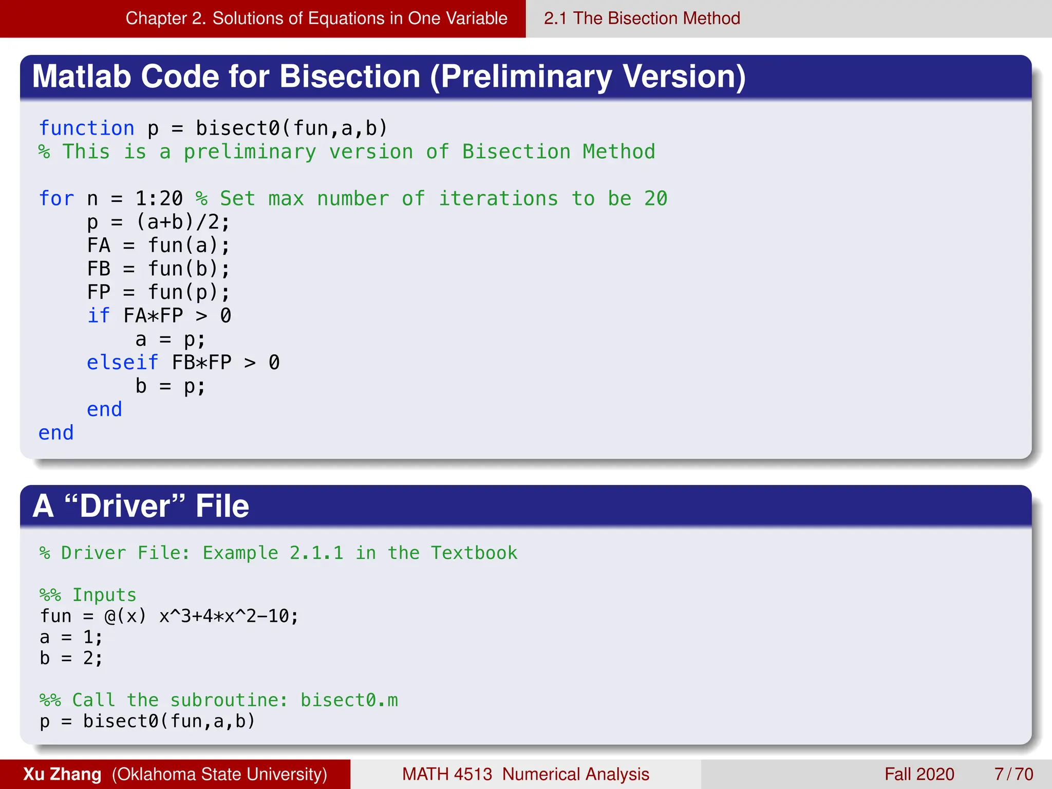
Matlab Code for Bisection (Preliminary Version)
8/21/19 5:28 PM /Users/xuzhang/Dropbox/Teachi.../bisect0.m 1
function p = bisect0(fun,a,b)
% This is a preliminary version of Bisection Method
for n = 1:20 % Set max number of iterations to be 20
p = (a+b)/2;
FA = fun(a);
FB = fun(b);
FP = fun(p);
if FA*FP 0
a = p;
elseif FB*FP 0
b = p;
end
end
A “Driver” File
8/21/19 5:28 PM /Users/xuzhang/Dropbox/Teachi.../ex2_1_0.m 1 of 1
% Driver File: Example 2.1.1 in the Textbook
%% Inputs
fun = @(x) x^3+4*x^2-10;
a = 1;
b = 2;
%% Call the subroutine: bisect0.m
p = bisect0(fun,a,b)
Xu Zhang (Oklahoma State University) MATH 4513 Numerical Analysis Fall 2020 7 / 70
8.
Chapter 2. Solutionsof Equations in One Variable 2.1 The Bisection Method
After 20 iterations, we obtain the solution p ≈ 1.365229606628418.
To display more information from the whole iteration process, we
modify the MATLAB subroutine file.
Matlab Code for Bisection (Preliminary Version with more outputs)
8/21/19 5:39 PM /Users/xuzhang/Dropbox/Teachi.../bisect1.m 1 of 1
function p = bisect1(fun,a,b)
% This is a preliminary version of Bisection Method
% This version displays intermediate outputs nicely
disp('Bisection Methods')
disp('-----------------------------------------------------------------')
disp(' n a_n b_n p_n f(p_n)')
disp('-----------------------------------------------------------------')
formatSpec = '%2d % .9f % .9f % .9f % .9f n';
for n = 1:20 % Set max number of iterations to be 20
p = (a+b)/2;
FA = fun(a);
FB = fun(b);
FP = fun(p);
fprintf(formatSpec,[n,a,b,p,fun(p)]) % Printing output
if FA*FP 0
a = p;
elseif FB*FP 0
b = p;
end
end
Xu Zhang (Oklahoma State University) MATH 4513 Numerical Analysis Fall 2020 8 / 70
9.
Chapter 2. Solutionsof Equations in One Variable 2.1 The Bisection Method
Some Remarks on Bisection Method
To start, an interval [a, b] must be found with f(a) · f(b) 0.
Otherwise, there may be no solutions in that interval.
It is good to set a maximum iteration number “maxit”, in case the
the iteration enters an endless loop.
It is good to set a tolerance or stopping criteria to avoid
unnecessary computational effort, such as
1
bn − an
2
tol
2 |pn − pn+1| tol
3
|pn − pn+1|
|pn|
tol
4 |f(pn)| tol
Xu Zhang (Oklahoma State University) MATH 4513 Numerical Analysis Fall 2020 9 / 70
10.
Chapter 2. Solutionsof Equations in One Variable 2.1 The Bisection Method
A more robust Matlab code for Bisection method
8/27/19 12:00 AM /Users/xuzhang/Dropbox/Teachi.../bisect.m 1 of 1
function [p,flag] = bisect(fun,a,b,tol,maxIt)
%% This is a more robust version of Bisection Method than bisect1.m
flag = 0; % Use a flag to tell if the output is reliable
if fun(a)*fun(b) 0 % Check f(a) and f(b) have different sign
error('f(a) and f(b) must have different signs');
end
disp('Bisection Methods')
disp('-----------------------------------------------------------------')
disp(' n a_n b_n p_n f(p_n)')
disp('-----------------------------------------------------------------')
formatSpec = '%2d % .9f % .9f % .9f % .9f n';
for n = 1:maxIt
p = (a+b)/2;
FA = fun(a);
FP = fun(p);
fprintf(formatSpec,[n,a,b,p,fun(p)]) % Printing output
if abs(FP) = 10^(-15) || (b-a)/2 tol
flag = 1;
break; % Break out the for loop.
else
if FA*FP 0
a = p;
else
b = p;
end
end
end
Xu Zhang (Oklahoma State University) MATH 4513 Numerical Analysis Fall 2020 10 / 70
11.
Chapter 2. Solutionsof Equations in One Variable 2.1 The Bisection Method
Example 2.
Use Bisection method to find a root of f(x) = x3 + 4x2 − 10 = 0 in the
interval [1, 2] that is accurate to at least within 10−4.
Solution.
We write a Matlab driver file for this test problem
8/14/18 2:17 PM /Users/zhang/Dropbox/Teaching.../ex2_1_1.
% Example 2.1.1 in the Textbook
fun = @(x) x^3+4*x^2-10;
a = 1;
b = 2;
tol = 1E-4;
maxIt = 40;
[p,flag] = bisect(fun,a,b,tol,maxIt);
In this driver file, we
specify all five inputs: fun, a, b, tol, maxIt
call the Bisection method code bisect.m.
Xu Zhang (Oklahoma State University) MATH 4513 Numerical Analysis Fall 2020 11 / 70
12.
Chapter 2. Solutionsof Equations in One Variable 2.1 The Bisection Method
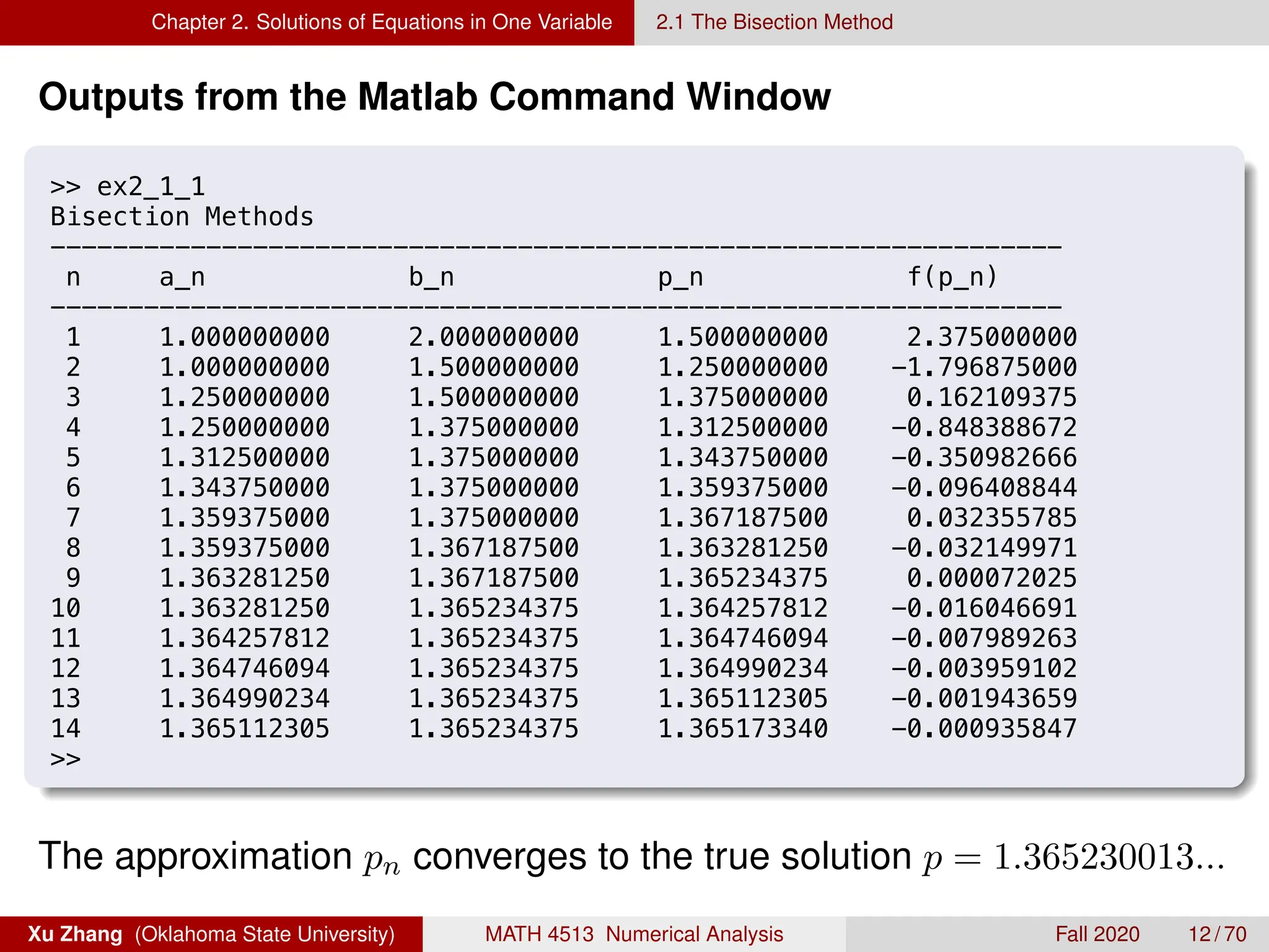
Outputs from the Matlab Command Window
8/27/19 12:08 AM MATLAB Command Window
ex2_1_1
Bisection Methods
-----------------------------------------------------------------
n a_n b_n p_n f(p_n)
-----------------------------------------------------------------
1 1.000000000 2.000000000 1.500000000 2.375000000
2 1.000000000 1.500000000 1.250000000 -1.796875000
3 1.250000000 1.500000000 1.375000000 0.162109375
4 1.250000000 1.375000000 1.312500000 -0.848388672
5 1.312500000 1.375000000 1.343750000 -0.350982666
6 1.343750000 1.375000000 1.359375000 -0.096408844
7 1.359375000 1.375000000 1.367187500 0.032355785
8 1.359375000 1.367187500 1.363281250 -0.032149971
9 1.363281250 1.367187500 1.365234375 0.000072025
10 1.363281250 1.365234375 1.364257812 -0.016046691
11 1.364257812 1.365234375 1.364746094 -0.007989263
12 1.364746094 1.365234375 1.364990234 -0.003959102
13 1.364990234 1.365234375 1.365112305 -0.001943659
14 1.365112305 1.365234375 1.365173340 -0.000935847
The approximation pn converges to the true solution p = 1.365230013...
Xu Zhang (Oklahoma State University) MATH 4513 Numerical Analysis Fall 2020 12 / 70
13.
Chapter 2. Solutionsof Equations in One Variable 2.1 The Bisection Method
Theorem 3 (Convergence of Bisection Method).
Suppose that f ∈ C[a, b] and f(a) · f(b) 0. The Bisection method
generates a sequence {pn}∞
n=1 approximating a zero p of f with
|pn − p| ≤
b − a
2n
, when n ≥ 1.
Proof.
For n ≥ 1, we have p ∈ (an, bn) and
bn − an =
1
2n−1
(b − a).
Since pn = 1
2(an + bn) for all n ≥ 1, then
|pn − p| ≤
1
2
(bn − an) =
b − a
2n
.
Xu Zhang (Oklahoma State University) MATH 4513 Numerical Analysis Fall 2020 13 / 70
14.
Chapter 2. Solutionsof Equations in One Variable 2.1 The Bisection Method
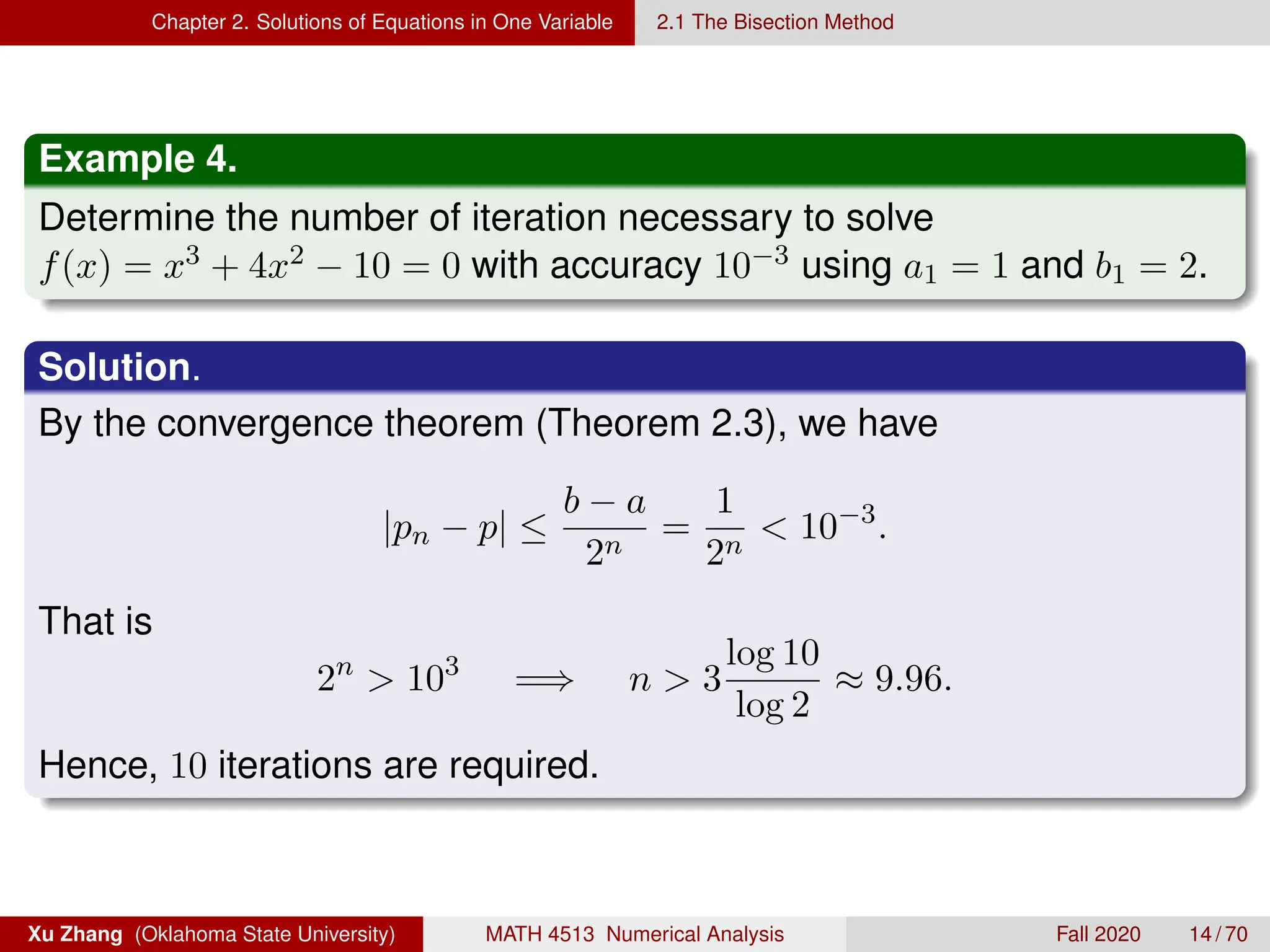
Example 4.
Determine the number of iteration necessary to solve
f(x) = x3 + 4x2 − 10 = 0 with accuracy 10−3 using a1 = 1 and b1 = 2.
Solution.
By the convergence theorem (Theorem 2.3), we have
|pn − p| ≤
b − a
2n
=
1
2n
10−3
.
That is
2n
103
=⇒ n 3
log 10
log 2
≈ 9.96.
Hence, 10 iterations are required.
Xu Zhang (Oklahoma State University) MATH 4513 Numerical Analysis Fall 2020 14 / 70
15.
Chapter 2. Solutionsof Equations in One Variable 2.2 Fixed-Point Iteration
2.2 Fixed-Point Iteration
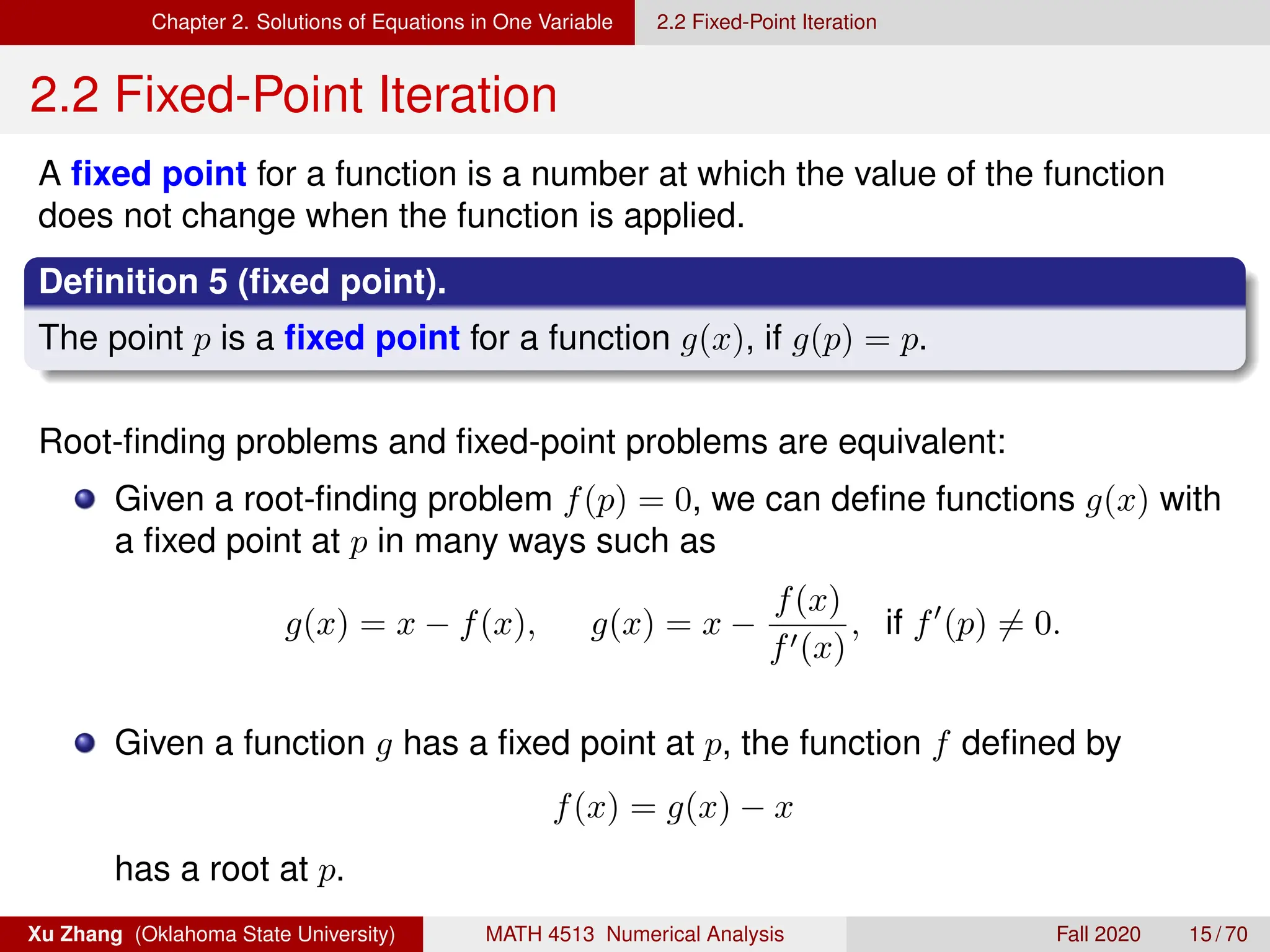
A fixed point for a function is a number at which the value of the function
does not change when the function is applied.
Definition 5 (fixed point).
The point p is a fixed point for a function g(x), if g(p) = p.
Root-finding problems and fixed-point problems are equivalent:
Given a root-finding problem f(p) = 0, we can define functions g(x) with
a fixed point at p in many ways such as
g(x) = x − f(x), g(x) = x −
f(x)
f0(x)
, if f0
(p) 6= 0.
Given a function g has a fixed point at p, the function f defined by
f(x) = g(x) − x
has a root at p.
Xu Zhang (Oklahoma State University) MATH 4513 Numerical Analysis Fall 2020 15 / 70
16.
Chapter 2. Solutionsof Equations in One Variable 2.2 Fixed-Point Iteration
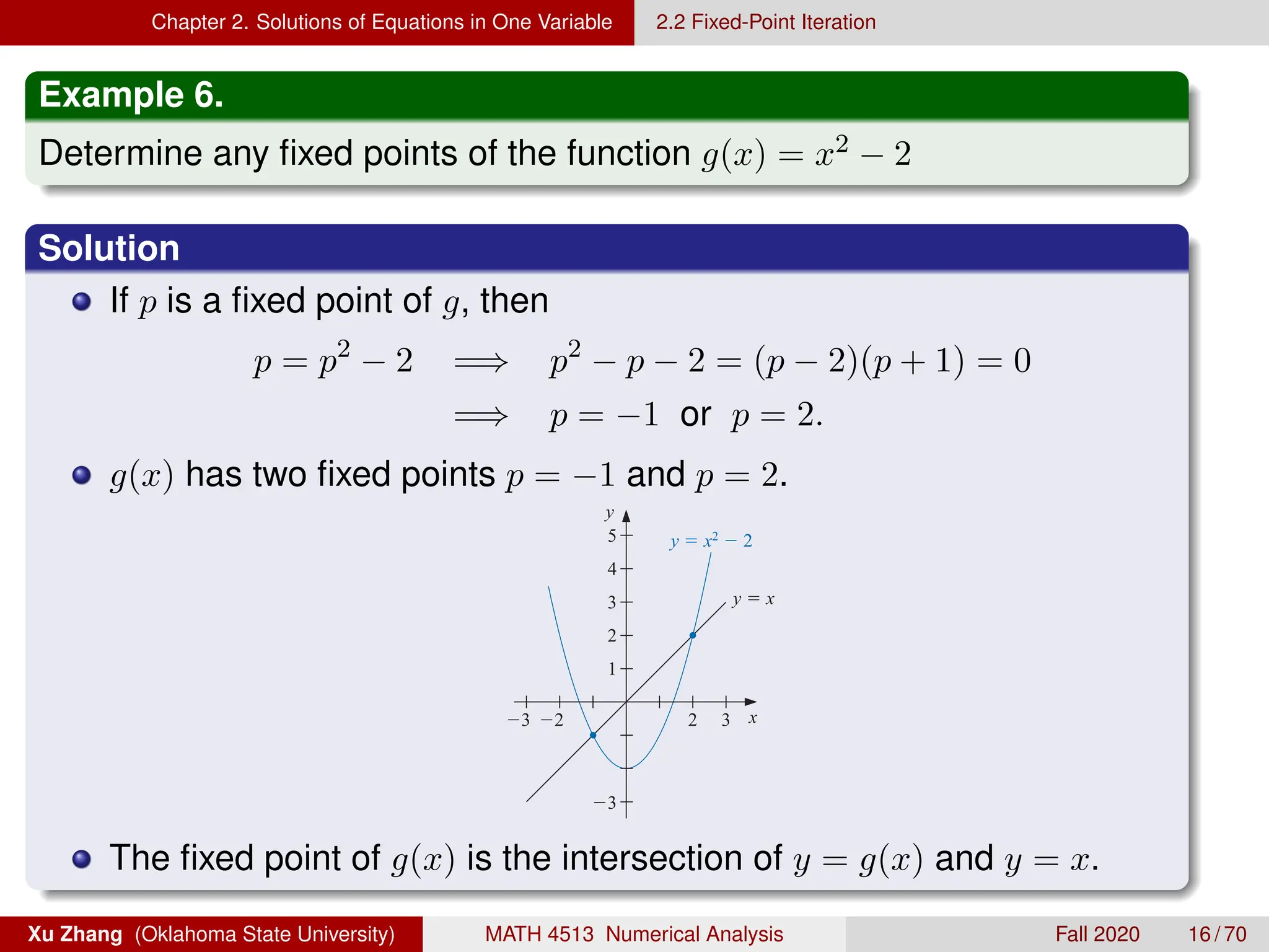
Example 6.
Determine any fixed points of the function g(x) = x2 − 2
Solution
If p is a fixed point of g, then
p = p2
− 2 =⇒ p2
− p − 2 = (p − 2)(p + 1) = 0
=⇒ p = −1 or p = 2.
g(x) has two fixed points p = −1 and p = 2.
2.2 Fixed-Point Iteration 57
Figure 2.3
y
x
3 2 2 3
1
3
2
3
4
5 y x2
2
y x
The following theorem gives sufficient conditions for the existence and uniqueness of
The fixed point of g(x) is the intersection of y = g(x) and y = x.
Xu Zhang (Oklahoma State University) MATH 4513 Numerical Analysis Fall 2020 16 / 70
17.
Chapter 2. Solutionsof Equations in One Variable 2.2 Fixed-Point Iteration
Theorem 7 (Sufficient Conditions for Fixed Points).
(i) (Existence) If g ∈ C[a, b] and g(x) ∈ [a, b] for all x ∈ [a, b], then g
has at least one fixed point in [a, b].
(ii) (Uniqueness) If, in addition, g0(x) exists and satisfies
|g0
(x)| ≤ k 1, for all x ∈ (a, b),
for some positive constant k, there is exactly one fixed-point in [a, b].
x
3 2 2 3
3
The following theorem gives sufficient conditions for the existence and uniqueness of
a fixed point.
Theorem 2.3 (i) If g ∈ C[a, b] and g(x) ∈ [a, b] for all x ∈ [a, b], then g has at least one fixed
point in [a, b].
(ii) If, in addition, g (x) exists on (a, b) and a positive constant k 1 exists with
|g (x)| ≤ k, for all x ∈ (a, b),
then there is exactly one fixed point in [a, b]. (See Figure 2.4.)
Figure 2.4
y
x
y x
y g(x)
p g(p)
a p b
a
b
Proof
(i) If g(a) = a or g(b) = b, then g has a fixed point at an endpoint. If not, then
g(a) a and g(b) b. The function h(x) = g(x)−x is continuous on [a, b], with
Note: the proof of existence uses the Intermediate Value Theorem, and
the proof of uniqueness uses the Mean Value Theorem.
Xu Zhang (Oklahoma State University) MATH 4513 Numerical Analysis Fall 2020 17 / 70
18.
Chapter 2. Solutionsof Equations in One Variable 2.2 Fixed-Point Iteration
Example 8.
Show that g(x) =
1
3
(x2
− 1) has a unique fixed-point on [−1, 1].
Proof (1/2)
(1. Existence). We show that g(x) has at least a fixed point p ∈ [−1, 1].
Taking the derivative,
g0
(x) =
2x
3
, only one critical point x = 0, g(0) = −
1
3
.
At endpoints, x = −1 and 1, we have g(−1) = 0, and g(1) = 0.
Then we have the global extreme values
min
x∈[−1,1]
g(x) = −
1
3
, and max
x∈[−1,1]
g(x) = 0.
Therefore, g(x) ∈ [−1
3 , 0] ⊂ [−1, 1]. By the first part of Theorem 2.7, the
function g has at least one fixed-point on [−1, 1].
Xu Zhang (Oklahoma State University) MATH 4513 Numerical Analysis Fall 2020 18 / 70
19.
Chapter 2. Solutionsof Equations in One Variable 2.2 Fixed-Point Iteration
Proof (2/2)
(2. Uniqueness). We show that g(x) has exactly one fixed point.
Note that
|g0
(x)| =
2x
3
≤
2
3
, ∀x ∈ (−1, 1).
By part (ii) of Theorem 2.7, g has a unique fixed-point on [−1, 1].
Remark
In fact, p =
3 −
√
13
2
is the fixed-point on the interval [−1, 1].
Xu Zhang (Oklahoma State University) MATH 4513 Numerical Analysis Fall 2020 19 / 70
20.
Chapter 2. Solutionsof Equations in One Variable 2.2 Fixed-Point Iteration
Remark
The function g has another fixed point q = 3+
√
13
2 on the interval
[3, 4]. However, it does not satisfy the hypotheses of Theorem 2.7
(why? exercise).
The hypotheses in Theorem 2.7 are sufficient but not necessary.
2.2 Fixed-Point Iteration 59
Figure 2.5
y
x
y
3
x2 1
y
3
x2 1
1
2
3
4
1 2 3 4
1
y x
y
x
1
2
3
4
1 2 3 4
1
y x
Xu Zhang (Oklahoma State University) MATH 4513 Numerical Analysis Fall 2020 20 / 70
21.
Chapter 2. Solutionsof Equations in One Variable 2.2 Fixed-Point Iteration
Fixed-Point Iteration
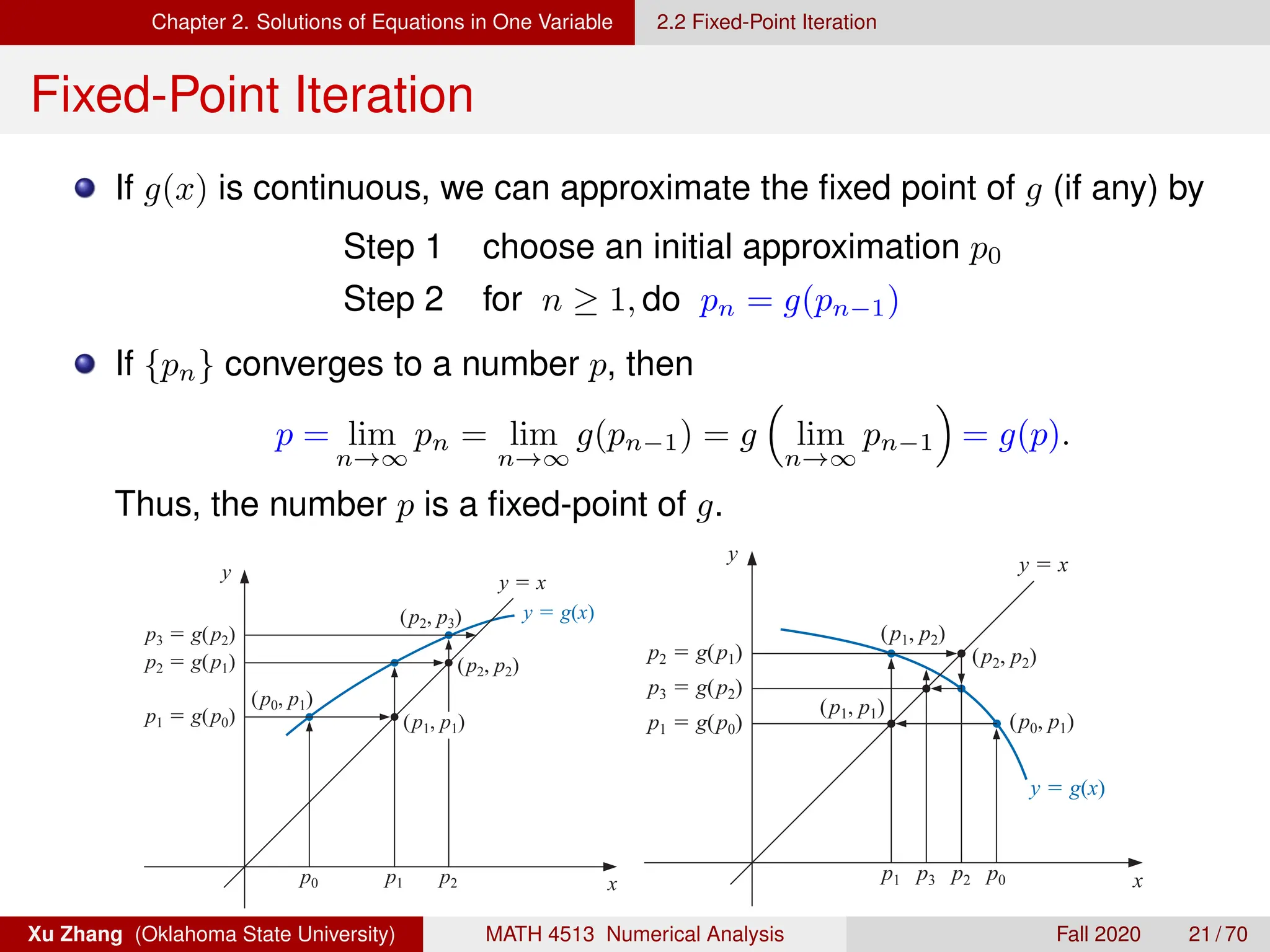
If g(x) is continuous, we can approximate the fixed point of g (if any) by
Step 1 choose an initial approximation p0
Step 2 for n ≥ 1, do pn = g(pn−1)
If {pn} converges to a number p, then
p = lim
n→∞
pn = lim
n→∞
g(pn−1) = g
lim
n→∞
pn−1
= g(p).
Thus, the number p is a fixed-point of g.
in One Variable
eration
itly determine the fixed point in Example 3 because we have no way to
equation p = g( p) = 3−p
. We can, however, determine approximations
t to any specified degree of accuracy. We will now consider how this can
ate the fixed point of a function g, we choose an initial approximation p0
sequence { pn}∞
n=0 by letting pn = g( pn−1), for each n ≥ 1. If the sequence
d g is continuous, then
p = lim
n→∞
pn = lim
n→∞
g( pn−1) = g
lim
n→∞
pn−1
= g( p),
x = g(x) is obtained. This technique is called fixed-point, or functional
ocedure is illustrated in Figure 2.7 and detailed in Algorithm 2.2.
x x
y
x
1)
g(x)
(b)
p0 p1 p2
y g(x)
(p2, p2)
(p0, p1)
(p2, p3)
p1 g(p0)
p3 g(p2)
y x
p2 g(p1)
(p1, p1)
60 C H A P T E R 2 Solutions of Equations in One Variable
Fixed-Point Iteration
We cannot explicitly determine the fix
solve for p in the equation p = g( p) =
to this fixed point to any specified degr
be done.
To approximate the fixed point of a
and generate the sequence { pn}∞
n=0 by le
converges to p and g is continuous, then
p = lim
n→∞
pn = lim
n→∞
g
and a solution to x = g(x) is obtained.
iteration. The procedure is illustrated i
Figure 2.7
x
y
y x
p2 g(p1)
p3 g(p2)
p1 g(p0)
(p1, p2)
(p2, p2)
(p0, p1)
y g(x)
(p1, p1)
p1 p3 p2 p0
(a)
p1 g
p3 g
p2 g
Xu Zhang (Oklahoma State University) MATH 4513 Numerical Analysis Fall 2020 21 / 70
22.
Chapter 2. Solutionsof Equations in One Variable 2.2 Fixed-Point Iteration
Matlab Code of Fixed-Point Iteration
8/28/19 11:02 PM /Users/xuzhang/Dropbox/Te.../fixedpoi
function [p,flag] = fixedpoint(fun,p0,tol,maxIt)
n = 1; flag = 0; % Initialization
disp('Fixed Point Iteration')
disp('----------------------------------')
disp(' n p f(p_n)')
disp('----------------------------------')
formatSpec = '%2d % .9f % .9f n';
fprintf(formatSpec,[n-1,p0,fun(p0)]) % printing output
while n = maxIt
p = fun(p0);
fprintf(formatSpec,[n,p,fun(p)]) % printing output
if abs(p-p0) tol
flag = 1;
break;
else
n = n+1;
p0 = p;
end
end
Note: unlike Bisection method, we don’t need to input an interval [a, b]
to start the fixed-point iteration, but we need an initial guess p0.
Xu Zhang (Oklahoma State University) MATH 4513 Numerical Analysis Fall 2020 22 / 70
23.
Chapter 2. Solutionsof Equations in One Variable 2.2 Fixed-Point Iteration
Example 9.
The equation x3 + 4x2 − 10 = 0 has a unique solution in [1, 2]. There
are many ways to change the equation to a fixed-point problem
x = g(x). For example,
g1(x) = x − x3 − 4x2 + 10
g2(x) =
r
10
x
− 4x
g3(x) =
1
2
√
10 − x3
g4(x) =
r
10
4 + x
g5(x) = x −
x3 + 4x2 − 10
3x2 + 8x
Which one is better?
Xu Zhang (Oklahoma State University) MATH 4513 Numerical Analysis Fall 2020 23 / 70
24.
Chapter 2. Solutionsof Equations in One Variable 2.2 Fixed-Point Iteration
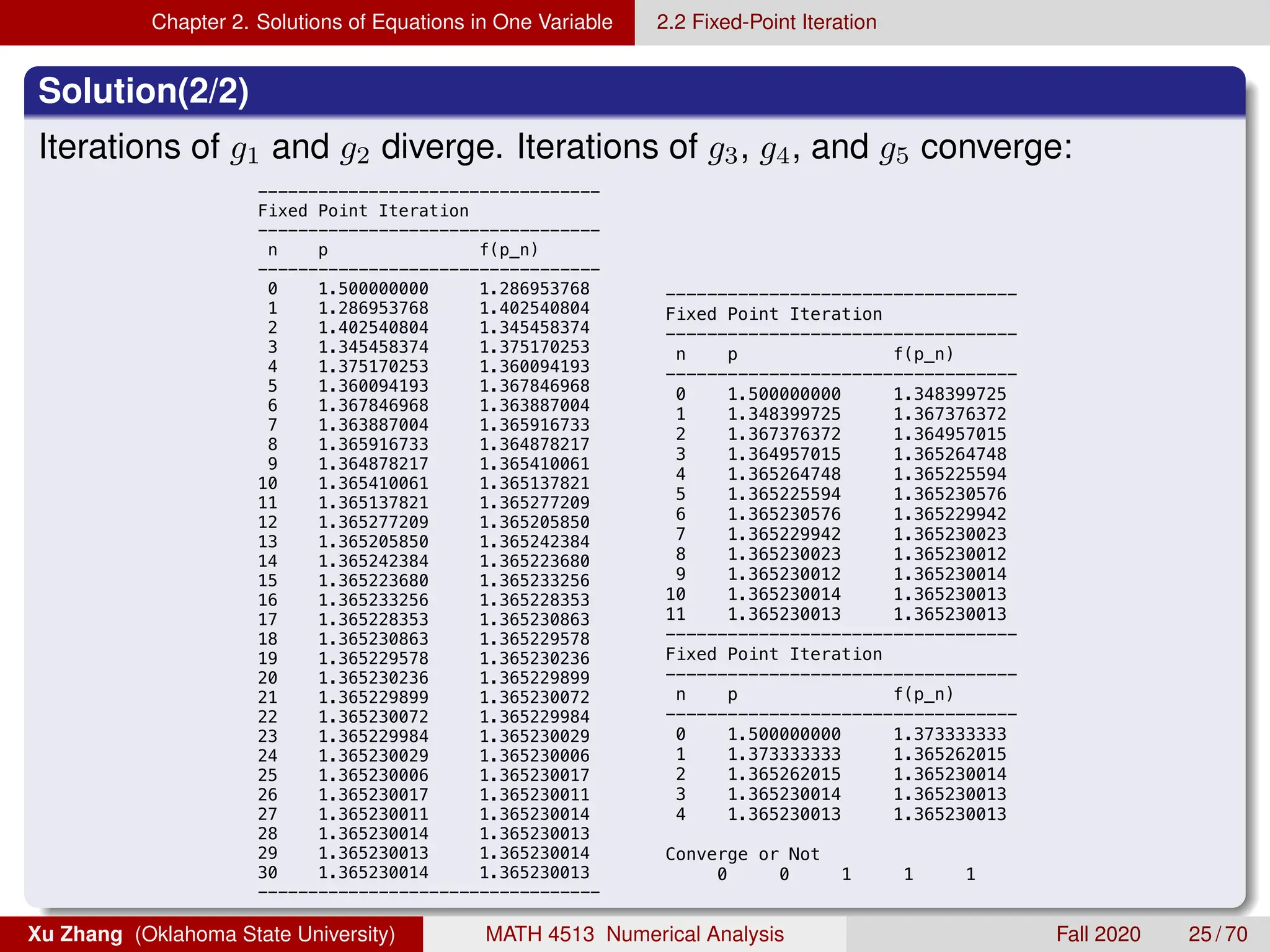
Solution(1/2): Write a Matlab driver file for this example
8/28/19 11:11 PM /Users/xuzhang/Dropbox/Teach.../ex2_2_1.m 1
% Example 2.2.1 in the Textbook
% Compare the convergence of fixed point iteration for five functions
clc % clear the command window
fun = @(x) x^3+4*x^2-10;
funG1 = @(x) x-x^3-4*x^2+10;
funG2 = @(x) sqrt(10/x-4*x);
funG3 = @(x) (1/2)*sqrt(10-x^3);
funG4 = @(x) sqrt(10/(4+x));
funG5 = @(x) x-(x^3+4*x^2-10)/(3*x^2+8*x);
p0 = 1.5;
tol = 1E-9;
maxIt = 40;
disp('--------------Test #1--------------')
[p1,flag1] = fixedpoint(funG1,p0,tol,maxIt);
disp('--------------Test #2--------------')
[p2,flag2] = fixedpoint(funG2,p0,tol,maxIt);
disp('--------------Test #3--------------')
[p3,flag3] = fixedpoint(funG3,p0,tol,maxIt);
disp('--------------Test #4--------------')
[p4,flag4] = fixedpoint(funG4,p0,tol,maxIt);
disp('--------------Test #5--------------')
[p5,flag5] = fixedpoint(funG5,p0,tol,maxIt);
disp(' ')
disp('Converge or Not')
disp([flag1,flag2,flag3,flag4,flag5])
Xu Zhang (Oklahoma State University) MATH 4513 Numerical Analysis Fall 2020 24 / 70
Chapter 2. Solutionsof Equations in One Variable 2.2 Fixed-Point Iteration
Questions
Why do iterations g1 and g2 diverge? but g3, g4, and g5 converge?
Why do g4 and g5 converge more rapidly than g3?
Theorem 10 (Fixed-Point Theorem).
Let g ∈ C[a, b] and g(x) ∈ [a, b] for all x ∈ [a, b]. Suppose that g0
exists on
(a, b) and that a constant 0 k 1 exists with
|g0
(x)| ≤ k 1, ∀x ∈ (a, b).
Then for any number p0 ∈ [a, b], the sequence
pn = g(pn−1), n ≥ 1
converges to the unique fixed point p in [a, b].
Xu Zhang (Oklahoma State University) MATH 4513 Numerical Analysis Fall 2020 26 / 70
27.
Chapter 2. Solutionsof Equations in One Variable 2.2 Fixed-Point Iteration
Proof
The function g satisfies the hypotheses of Theorem 2.7, thus g has a
unique fixed-point p in [a, b]. By Mean Value Theorem,
|pn − p| = |g(pn−1) − g(p)|
= |g0
(ξ)||pn−1 − p|
≤ k|pn−1 − p|
≤ · · ·
≤ kn
|p0 − p|.
Since 0 k 1, then
lim
n→∞
|pn − p| ≤ lim
n→∞
kn
|p0 − p| = 0.
Hence, the sequence {pn} converge to p.
Xu Zhang (Oklahoma State University) MATH 4513 Numerical Analysis Fall 2020 27 / 70
28.
Chapter 2. Solutionsof Equations in One Variable 2.2 Fixed-Point Iteration
Remark
The rate of convergence of the fixed-point iteration depends on the
factor k. The smaller the value of k, the faster the convergence.
To be more precise, we have the following error bounds (Corollary
2.5 in textbook)
|pn − p| ≤ kn
max{p0 − a, b − p0}.
and
|pn − p| ≤
kn
1 − k
|p1 − p0|.
We will see more in Section 2.4.
Xu Zhang (Oklahoma State University) MATH 4513 Numerical Analysis Fall 2020 28 / 70
29.
Chapter 2. Solutionsof Equations in One Variable 2.2 Fixed-Point Iteration
Proof (read if you like)
Since p ∈ [a, b], then
|pn − p| ≤ kn
|p0 − p| ≤ kn
max{p0 − a, b − p0}.
For n ≥ 1,
|pn+1 − pn| = |g(pn) − g(pn−1)| ≤ k|pn − pn−1| ≤ · · · ≤ kn
|p1 − p0|.
For m ≥ n ≥ 1,
|pm − pn| = |pm − pm−1 + pm−1 − · · · − pn+1 + pn+1 − pn|
≤ |pm − pm−1| + |pm1 − pm−2| + · · · + |pn+1 − pn|
≤ km−1
|p1 − p0| + km−2
|p1 − p0| + · · · kn
|p1 − p0|
≤ kn
|p1 − p0| 1 + k + k2
+ km−n−1
.
Xu Zhang (Oklahoma State University) MATH 4513 Numerical Analysis Fall 2020 29 / 70
30.
Chapter 2. Solutionsof Equations in One Variable 2.2 Fixed-Point Iteration
Proof (2/2) (read if you like)
Let m → ∞, we have
|p − pn| = lim
m→∞
|pm − pn|
≤ lim
m→∞
kn
|p1 − p0| 1 + k + k2
+ km−n−1
= kn
|p1 − p0|
∞
X
i=0
ki
=
kn
1 − k
|p1 − p0|.
The last equality is because of the convergence of geometric series
when 0 k 1.
Xu Zhang (Oklahoma State University) MATH 4513 Numerical Analysis Fall 2020 30 / 70
31.
Chapter 2. Solutionsof Equations in One Variable 2.2 Fixed-Point Iteration
A revisit of the fixed-point schemes g1 to g5 in Example 2.9.
For g1(x) = x − x3 − 4x2 + 10, we know that
g1(1) = 6, and g2(2) = −12,
so g1 does not map [1, 2] into itself. Moreover,
|g0
1(x)| = |1 − 3x2
− 8x| 1, for all x ∈ [1, 2].
There is no reason to expect convergence.
For g2(x) =
r
10
x
− 4x, it does not map [1, 2] into [1, 2]. Also, there
is no interval containing the fixed point p ≈ 1.365 such that
|g0
2(x)| 1, because |g0
2(p)| ≈ 3.4 1. There is no reason to
expect it to converge.
Xu Zhang (Oklahoma State University) MATH 4513 Numerical Analysis Fall 2020 31 / 70
32.
Chapter 2. Solutionsof Equations in One Variable 2.2 Fixed-Point Iteration
A revisit of the fixed-point schemes g1 to g5 in Example 2.9.
For g3(x) =
1
2
√
10 − x3, we have
g0
3(x) = −
3
4
x2
(10 − x3
)−1/2
0, on [1, 2]
so g3 is strictly decreasing on [1, 2]. If we start with p0 = 1.5, it suffices to
consider the interval [1, 1.5]. Also note that
1 1.28 ≈ g3(1.5) ≤ g3(x) ≤ g3(1) = 1.5,
so g3 maps [1, 1.5] into itself. Moreover, it is also true that
|g0
3(x)| ≤ g0
3(1.5) ≈ 0.66,
on the interval [1, 1.5], so Theorem 2.10 guarantees its convergence.
(k ≈ 0.66)
Xu Zhang (Oklahoma State University) MATH 4513 Numerical Analysis Fall 2020 32 / 70
33.
Chapter 2. Solutionsof Equations in One Variable 2.2 Fixed-Point Iteration
A revisit of the fixed-point schemes g1 to g5 in Example 2.9.
For g4(x) =
r
10
4 + x
, it maps [1, 2] into itself. Moreover,
|g0
4(x)| ≤ |
√
10
2
(4+x)−3/2
| ≤
√
10
2
·5−3/2
=
1
5
√
2
0.15, for all x ∈ [1, 2].
So g4 converges much more rapidly than g3 (k ≈ 0.15).
For g5(x) = x −
x3
+ 4x2
− 10
3x2 + 8x
, it converges much more rapidly than
other choices. This choice of the g5(x) is in fact the Newton’s Method,
and we will see where this choice came from and why it is so effective in
the next section.
Xu Zhang (Oklahoma State University) MATH 4513 Numerical Analysis Fall 2020 33 / 70
34.
Chapter 2. Solutionsof Equations in One Variable 2.2 Fixed-Point Iteration
Concluding Remark
Question How can we find a fixed-point problem that produces a
sequence that reliably and rapidly converges to a solution
to a given root-finding problem?
Answer Manipulate the root-finding problem into a fixed point
problem that satisfies the conditions of Fixed-Point
Theorem (Theorem 2.10) and has a derivative that is as
small as possible near the fixed point.
Xu Zhang (Oklahoma State University) MATH 4513 Numerical Analysis Fall 2020 34 / 70
35.
Chapter 2. Solutionsof Equations in One Variable 2.3 Newton’s Method and Its Extensions
2.3 Newton’s Method and Its Extensions
In this section, we introduce one of the most powerful and well-known
numerical methods for root-finding problems, namely Newton’s method
(or Newton-Raphson method).
Suppose f ∈ C2
[a, b]. Let p0 ∈ (a, b) be an approximation to a root p such
that f0
(p0) 6= 0. Assume that |p − p0| is small. By Taylor expansion,
f(p) = f(p0) + (p − p0)f0
(p0) +
(p − p0)2
2
f00
(ξ)
where ξ is between p0 and p.
Since f(p) = 0,
0 = f(p0) + (p − p0)f0
(p0) +
(p − p0)2
2
f00
(ξ)
Since p − p0 is small, we drop the high-order term involving (p − p0)2
,
0 ≈ f(p0) + (p − p0)f0
(p0) =⇒ p ≈ p0 −
f(p0)
f0(p0)
≡ p1.
Xu Zhang (Oklahoma State University) MATH 4513 Numerical Analysis Fall 2020 35 / 70
36.
Chapter 2. Solutionsof Equations in One Variable 2.3 Newton’s Method and Its Extensions
Newton’s Method
Given an initial approximation p0, generate a sequence {pn}∞
n=0 by
pn = pn−1 −
f(pn−1)
f0(pn−1)
, for n ≥ 1.
68 C H A P T E R 2 Solutions of Equations in One Variable
Figure 2.8
x
x
y
(p0, f(p0))
(p1, f(p1))
p0
p1
p2
p
Slope f(p0)
y f(x)
Slope f(p1)
ALGORITHM
2.3
Newton’s
To find a solution to f (x) = 0 given an initial approximation p0:
INPUT initial approximation p0; tolerance TOL; maximum number of iterations N0.
OUTPUT approximate solution p or message of failure.
Note that pn is the x-intercept of the tangent line to f at (pn−1, f(pn−1)).
An animation:
https://upload.wikimedia.org/wikipedia/commons/e/e0/NewtonIteration_Ani.gif
Xu Zhang (Oklahoma State University) MATH 4513 Numerical Analysis Fall 2020 36 / 70
37.
Chapter 2. Solutionsof Equations in One Variable 2.3 Newton’s Method and Its Extensions
To program the Newton’s method, the inputs should contain f, p0, tol,
maxit, as used in the fixed-point methods.
In addition, we also need to include the derivative f0
as an input.
Matlab Code of Newton’s Method
9/3/18 11:41 PM /Users/xuzhang/Dropbox/Teachin.../newton.m 1 of 1
function [p,flag] = newton(fun,Dfun,p0,tol,maxIt)
n = 0; flag = 0; % Initializaiton
disp('-----------------------------------')
disp('Newton Method')
disp('-----------------------------------')
disp(' n p_n f(p_n)')
disp('-----------------------------------')
formatSpec = '%2d %.10f % .10f n';
fprintf(formatSpec,[n,p0,fun(p0)])
while n=maxIt
p = p0 - fun(p0)/Dfun(p0);
if abs(p-p0) tol
flag = 1; break;
else
n = n+1; p0 = p;
end
fprintf(formatSpec,[n,p,fun(p)])
end
Xu Zhang (Oklahoma State University) MATH 4513 Numerical Analysis Fall 2020 37 / 70
38.
Chapter 2. Solutionsof Equations in One Variable 2.3 Newton’s Method and Its Extensions
Example 11.
Let f(x) = cos(x) − x. Approximate a root of f using (i) the fixed-point
method with g(x) = cos(x) and (ii) Newton’s method.
Solution (1/3)
(i). Using the fixed-point function g(x) = cos(x), we can start the
fixed-point iteration with p0 = π/4.
g( pn−1) = pn−1 −
f ( pn−1)
f ( pn−1)
, for n ≥ 1. (2.11)
In fact, this is the functional iteration technique that was used to give the rapid convergence
we saw in column (e) of Table 2.2 in Section 2.2.
It is clear from Equation (2.7) that Newton’s method cannot be continued if f ( pn−1) =
0 for some n. In fact, we will see that the method is most effective when f is bounded away
from zero near p.
Example 1 Consider the function f (x) = cos x−x = 0. Approximate a root of f using (a) a fixed-point
method, and (b) Newton’s Method
Solution (a) A solution to this root-finding problem is also a solution to the fixed-point
problem x = cos x, and the graph in Figure 2.9 implies that a single fixed-point p lies in
[0, π/2].
Figure 2.9
y
x
y x
y cos x
1
1
e in the
on is in
degrees. This
ase unless
Xu Zhang (Oklahoma State University) MATH 4513 Numerical Analysis Fall 2020 38 / 70
39.
Chapter 2. Solutionsof Equations in One Variable 2.3 Newton’s Method and Its Extensions
Solution (2/3)
(ii). To apply Newton’s method, we calculate f0(x) = − sin(x) − 1. We
again start with p0 = π/4.
A MATLAB driver file for this example
9/2/19 11:23 AM /Users/xuzhang/Dropbox/Teachi.../ex2_3_1.m
% Example 2.3.1 in the Textbook
fun = @(x) cos(x)-x; % Function f(x)
Dfun = @(x) -sin(x)-1; % Derivative of f(x)
funF = @(x) cos(x); % Function for fixed point iteration
tol = 1E-10;
maxIt = 20;
%% Fixed-Point Iteration
p0 = pi/4;
[pF,flagF] = fixedpoint(funF,p0,tol,maxIt);
disp(' ')
%% Newton Method
p0 = pi/4;
[p,flag] = newton(fun,Dfun,p0,tol,maxIt);
disp(' ')
Xu Zhang (Oklahoma State University) MATH 4513 Numerical Analysis Fall 2020 39 / 70
40.
Chapter 2. Solutionsof Equations in One Variable 2.3 Newton’s Method and Its Extensions
Solution (3/3)
Home License -- for personal use only. Not for government,
academic, research, commercial, or other organizational use.
ex2_3_1
Fixed Point Iteration
----------------------------------
n p f(p_n)
----------------------------------
0 0.785398163 0.707106781
1 0.707106781 0.760244597
2 0.760244597 0.724667481
3 0.724667481 0.748719886
4 0.748719886 0.732560845
5 0.732560845 0.743464211
6 0.743464211 0.736128257
7 0.736128257 0.741073687
8 0.741073687 0.737744159
9 0.737744159 0.739987765
10 0.739987765 0.738476809
11 0.738476809 0.739494771
12 0.739494771 0.738809134
13 0.738809134 0.739271021
14 0.739271021 0.738959904
15 0.738959904 0.739169483
16 0.739169483 0.739028311
17 0.739028311 0.739123408
18 0.739123408 0.739059350
19 0.739059350 0.739102501
20 0.739102501 0.739073434
-----------------------------------
Newton Method
-----------------------------------
n p_n f(p_n)
-----------------------------------
0 0.7853981634 -0.0782913822
1 0.7395361335 -0.0007548747
2 0.7390851781 -0.0000000751
3 0.7390851332 -0.0000000000
Comparing with the Fixed-point iteration, Newton method gives excellent
approximation with only three iterations.
Xu Zhang (Oklahoma State University) MATH 4513 Numerical Analysis Fall 2020 40 / 70
41.
Chapter 2. Solutionsof Equations in One Variable 2.3 Newton’s Method and Its Extensions
Remarks on Newton’s Method
Newton’s method can provide extremely accurate
approximations with very few iterations.
Newton’s method requires the initial approximation to be
sufficiently accurate.
In practical applications, an initial approximation can be obtained
by other methods, such as bisection method. After the
approximation is sufficient accurate, Newton’s method is applied
for rapid convergence.
Newton’s method requires evaluation of the derivative f0 at each
step. Usually f0 is far more difficult to calculate than f.
Xu Zhang (Oklahoma State University) MATH 4513 Numerical Analysis Fall 2020 41 / 70
42.
Chapter 2. Solutionsof Equations in One Variable 2.3 Newton’s Method and Its Extensions
Example 12.
Player A will shut out (win by a score of 21-0) player B in a game of
racquetball with probability
P =
1 + p
2
p
1 − p + p2
21
,
where p denotes the probability A will win any specific rally
(independent of the server). Determine the minimum value of p that
will ensure that player A will shut out player B in at least half the
matches they play.
Xu Zhang (Oklahoma State University) MATH 4513 Numerical Analysis Fall 2020 42 / 70
43.
Chapter 2. Solutionsof Equations in One Variable 2.3 Newton’s Method and Its Extensions
Solution
The player A winning at least half of the matches means P is at
least 0.5. We consider the root-finding problem
f(p) =
1 + p
2
p
1 − p + p2
21
− 0.5.
The derivative f0 is (verify by yourself)
f0
(p) =
1
2
p
1 − p + p2
21
+
21
2
(1+p)
p
1 − p + p2
20
1 − p2
(1 − p + p2)2
.
Using Newton’s method with p0 = 0.75, and
pn = pn−1 −
f(pn−1)
f0(pn−1)
, for n ≥ 1
we find that p ≈ 0.8423 in three iterations.
Xu Zhang (Oklahoma State University) MATH 4513 Numerical Analysis Fall 2020 43 / 70
44.
Chapter 2. Solutionsof Equations in One Variable 2.3 Newton’s Method and Its Extensions
In last example, we see that the finding the derivative f0(x) is not
easy, and the evaluation of f0(x) also requires more arithmetic
operations than the evaluation of f(x) itself.
To circumvent this problem, we introduce a variation of Newton’s
method that does require the evaluation of derivative f0.
Recall that in Newton’s method we have
pn = pn−1 −
f(pn−1)
f0(pn−1)
, for n ≥ 1
By the definition of derivative,
f0
(pn−1) = lim
x→pn−1
f(x) − f(pn−1)
x − pn−1
≈
f(pn−2) − f(pn−1)
pn−2 − pn−1
since pn−2 is close to pn−1.
Xu Zhang (Oklahoma State University) MATH 4513 Numerical Analysis Fall 2020 44 / 70
45.
Chapter 2. Solutionsof Equations in One Variable 2.3 Newton’s Method and Its Extensions
Secant Method
Replacing the derivative f0(pn−1) in the Newton’s formula by the
difference quotient, we have
pn = pn−1 −
f(pn−1)
f0(pn−1)
≈ pn−1 −
f(pn−1)
f(pn−2) − f(pn−1)
pn−2 − pn−1
= pn−1 −
f(pn−1)(pn−2 − pn−1)
f(pn−2) − f(pn−1)
n ≥ 2.
Xu Zhang (Oklahoma State University) MATH 4513 Numerical Analysis Fall 2020 45 / 70
46.
Chapter 2. Solutionsof Equations in One Variable 2.3 Newton’s Method and Its Extensions
Secant Method
Given initial approximations p0 and p1, generate a sequence {pn}∞
n=0
by
pn = pn−1 −
f(pn−1)(pn−2 − pn−1)
f(pn−2) − f(pn−1)
, n ≥ 2.
Remark
The Secant method requires two initial approximations.
However, it does not require the evaluation of the derivative.
Xu Zhang (Oklahoma State University) MATH 4513 Numerical Analysis Fall 2020 46 / 70
47.
Chapter 2. Solutionsof Equations in One Variable 2.3 Newton’s Method and Its Extensions
An illustration of Secant method
Figure 2.11
y y
y f(x)
p0 p1
p2 p3
p0
p4
Secant Method Method o
x
Copyright 2010 Cengage Learning. All Rights Reserved. May not be copied, scanned, or duplicated, in whole or in part. Due to electronic rights, some third p
Editorial review has deemed that any suppressed content does not materially affect the overall learning experience. Cengage Learning reserves the right to remove
Starting with two initial approximations p0 and p1, the value p2 is
the x-intercept of the line joining (p0, f(p0)) and (p1, f(p1)).
The approximation p3 is the x-intercept of the line joining
(p1, f(p1)) and (p2, f(p2)) and so on.
Xu Zhang (Oklahoma State University) MATH 4513 Numerical Analysis Fall 2020 47 / 70
48.
Chapter 2. Solutionsof Equations in One Variable 2.3 Newton’s Method and Its Extensions
Matlab Code of Secant Method
9/4/18 12:36 AM /Users/xuzhang/Dropbox/Teachin..
function [p,flag] = secant(fun,p0,p1,tol,maxIt)
n = 1; flag = 0; % Initializaiton
q0 = fun(p0); q1 = fun(p1);
disp('-----------------------------------')
disp('Secant Method')
disp('-----------------------------------')
disp(' n p_n f(p_n)')
disp('-----------------------------------')
formatSpec = '%2d %.10f % .10f n';
fprintf(formatSpec,[n-1,p0,fun(p0)])
fprintf(formatSpec,[n,p1,fun(p1)])
while n=maxIt
p = p1 - q1*(p1-p0)/(q1-q0);
if abs(p-p0) tol
flag = 1; break;
else
n = n+1;
p0 = p1; q0 = q1; p1 = p; q1 = fun(p);
end
fprintf(formatSpec,[n,p,fun(p)])
end
Xu Zhang (Oklahoma State University) MATH 4513 Numerical Analysis Fall 2020 48 / 70
49.
Chapter 2. Solutionsof Equations in One Variable 2.3 Newton’s Method and Its Extensions
Example 13.
Use the Secant method for find a solution to x = cos(x), and compare
with the approximation with those given from Newton’s method.
Solution (1/2)
Write a MATLAB driver file
9/4/18 12:37 AM /Users/xuzhang/Dropbox/Teachi...
% Example 2.3.2 in the Textbook
fun = @(x) cos(x)-x;
Dfun = @(x) -sin(x)-1;
tol = 1E-10;
maxIt = 40;
%% Newton
p0 = pi/4;
[pN,flagN] = newton(fun,Dfun,p0,tol,maxIt);
disp(' ')
%% Secant
p0 = 0.5; p1 = pi/4;
[pS,flagS] = secant(fun,p0,p1,tol,maxIt);
disp(' ')
Xu Zhang (Oklahoma State University) MATH 4513 Numerical Analysis Fall 2020 49 / 70
50.
Chapter 2. Solutionsof Equations in One Variable 2.3 Newton’s Method and Its Extensions
Solution (2/2)
9/4/18 12:38 AM MATLAB Command Window 1 of 1
ex2_3_2
-----------------------------------
Newton Method
-----------------------------------
n p_n f(p_n)
-----------------------------------
0 0.7853981634 -0.0782913822
1 0.7395361335 -0.0007548747
2 0.7390851781 -0.0000000751
3 0.7390851332 -0.0000000000
-----------------------------------
Secant Method
-----------------------------------
n p_n f(p_n)
-----------------------------------
0 0.5000000000 0.3775825619
1 0.7853981634 -0.0782913822
2 0.7363841388 0.0045177185
3 0.7390581392 0.0000451772
4 0.7390851493 -0.0000000270
5 0.7390851332 0.0000000000
6 0.7390851332 0.0000000000
Secant method requires 5 iterations comparing with 3 iteration
used in Newton’s method.
Xu Zhang (Oklahoma State University) MATH 4513 Numerical Analysis Fall 2020 50 / 70
51.
Chapter 2. Solutionsof Equations in One Variable 2.3 Newton’s Method and Its Extensions
Example 14.
A revisit of Example (Recquetball Winning Probability) use Secant
method.
Solution
The root-finding problem is
f(p) =
1 + p
2
p
1 − p + p2
21
− 0.5.
Use Secant method with p0 = 0.5, and p1 = 1, we can find
p ≈ 0.8423 within accuracy of 10−5 in five iterations.
Remark
Newton’s method uses three iterations to reach this accuracy.
However, it requires evaluations of the derivative f0.
Xu Zhang (Oklahoma State University) MATH 4513 Numerical Analysis Fall 2020 51 / 70
52.
Chapter 2. Solutionsof Equations in One Variable 2.3 Newton’s Method and Its Extensions
Remark
Secant Method converges slightly slower than Newton Method,
but much faster than other Fixed-point iterations.
Newton’s method or the Secant method is often used to refine an
answer obtained by another technique, such as the Bisection
method, since these methods require good first approximations
but generally give rapid convergence.
Xu Zhang (Oklahoma State University) MATH 4513 Numerical Analysis Fall 2020 52 / 70
53.
Chapter 2. Solutionsof Equations in One Variable 2.4 Error Analysis for Iterative Methods
2.4 Error Analysis for Iterative Methods
In this section we investigate the order of convergence of iteration
schemes.
For example, the following sequences all converge to 0 as n → ∞
1
n
,
1
n2
,
1
en
,
1
n!
.
Clearly, the “speed” of the convergence is different.
We will develop a procedure for measuring how rapidly a
sequence converges.
Xu Zhang (Oklahoma State University) MATH 4513 Numerical Analysis Fall 2020 53 / 70
54.
Chapter 2. Solutionsof Equations in One Variable 2.4 Error Analysis for Iterative Methods
Definition 15 (Order of Convergence).
Suppose {pn}∞
n=0 is a sequence that converges to p, with pn 6= p for all n.
If lim
n→∞
|pn+1 − p|
|pn − p|
= λ, where λ ∈ (0, 1), then {pn} is said to converge
linearly, with asymptotic error constant λ.
If lim
n→∞
|pn+1 − p|
|pn − p|
= 0, then {pn} is said to converge superlinearly.
If lim
n→∞
|pn+1 − p|
|pn − p|
= 1, then {pn} is said to converge sublinearly.
Xu Zhang (Oklahoma State University) MATH 4513 Numerical Analysis Fall 2020 54 / 70
55.
Chapter 2. Solutionsof Equations in One Variable 2.4 Error Analysis for Iterative Methods
Remark
To further distinguish superlinear convergences, we say the sequence
{pn} converges to p of order α 1 if
lim
n→∞
|pn+1 − p|
|pn − p|α
= M.
In particular,
α = 2 is called to quadratic convergence.
α = 3 is called to cubic convergence.
Xu Zhang (Oklahoma State University) MATH 4513 Numerical Analysis Fall 2020 55 / 70
56.
Chapter 2. Solutionsof Equations in One Variable 2.4 Error Analysis for Iterative Methods
Example 16.
The following sequences all converge to 0. Find the convergence order
of each sequence.
(a).
1
n
(b).
1
n2
(c).
1
2n
(d).
1
n!
(e).
1
22n
Solution (1/4)
(a). For
1
n
, the first few terms are 1,
1
2
,
1
3
,
1
4
,
1
5
, · · ·
lim
n→∞
|pn+1 − p|
|pn − p|
= lim
n→∞
1
n+1
1
n
= lim
n→∞
n
n + 1
= 1.
The sequence
1
n
converges to 0 sublinearly.
Xu Zhang (Oklahoma State University) MATH 4513 Numerical Analysis Fall 2020 56 / 70
57.
Chapter 2. Solutionsof Equations in One Variable 2.4 Error Analysis for Iterative Methods
Solution (2/4)
(b). For
1
n2
, the first few terms are 1,
1
4
,
1
9
,
1
16
,
1
25
, · · ·
lim
n→∞
|pn+1 − p|
|pn − p|
= lim
n→∞
1
(n+1)2
1
n2
= lim
n→∞
n2
(n + 1)2
= 1.
The sequence
1
n2
converges to 0 sublinearly.
(c). For
1
2n
, the first few terms are
1
2
,
1
4
,
1
8
,
1
16
,
1
32
, · · ·
lim
n→∞
|pn+1 − p|
|pn − p|
= lim
n→∞
1
2n+1
1
2n
= lim
n→∞
2n
2n+1
=
1
2
.
The sequence
1
2n
converges to 0 linearly.
Xu Zhang (Oklahoma State University) MATH 4513 Numerical Analysis Fall 2020 57 / 70
58.
Chapter 2. Solutionsof Equations in One Variable 2.4 Error Analysis for Iterative Methods
Solution (3/4)
(d). For
1
n!
, the first few terms are 1,
1
2
,
1
6
,
1
24
,
1
120
, · · ·
lim
n→∞
|pn+1 − p|
|pn − p|
= lim
n→∞
1
(n+1)!
1
n!
= lim
n→∞
n!
(n + 1)!
= lim
n→∞
1
n + 1
= 0.
The sequence
1
n!
converges to 0 superlinearly.
Note that for any a 1,
lim
n→∞
|pn+1 − p|
|pn − p|a
= lim
n→∞
(n!)a
(n + 1)!
= lim
n→∞
(n!)a−1
n + 1
→ ∞.
The convergence order of
1
n!
is barely 1, but not any more.
Xu Zhang (Oklahoma State University) MATH 4513 Numerical Analysis Fall 2020 58 / 70
59.
Chapter 2. Solutionsof Equations in One Variable 2.4 Error Analysis for Iterative Methods
Solution (4/4)
(e). For
1
22n
, the first few terms are
1
4
,
1
16
,
1
256
,
1
65536
,
1
4294967296
, · · ·
lim
n→∞
1
22n+1
1
22n
= lim
n→∞
22n
22n+1 = lim
n→∞
22n
22·2n = lim
n→∞
22n
(22n
)2
= lim
n→∞
1
22n = 0.
The sequence
1
22n
converges to 0 superlinearly.
Moreover, we note that
lim
n→∞
|pn+1 − p|
|pn − p|2
= lim
n→∞
1
22n+1
( 1
22n )2
= lim
n→∞
(22n
)2
22n+1 = lim
n→∞
(22n
)2
(22n
)2
= 1.
The sequence
1
22n
converges to 0 quadratically.
Xu Zhang (Oklahoma State University) MATH 4513 Numerical Analysis Fall 2020 59 / 70
60.
Chapter 2. Solutionsof Equations in One Variable 2.4 Error Analysis for Iterative Methods
Comparison of Linear and Quadratic Convergences
Table 2.7 illustrates the relative speed of convergence of the sequenc
Table 2.7 Linear Convergence Quadratic Convergence
Sequence { pn}∞
n=0 Sequence { p̃n}∞
n=0
n (0.5)n
(0.5)2n−1
1 5.0000 × 10⁻¹
5.0000 × 10⁻¹
2 2.5000 × 10⁻¹
1.2500 × 10⁻¹
3 1.2500 × 10⁻¹
7.8125 × 10⁻³
4 6.2500 × 10⁻²
3.0518 × 10⁻⁵
5 3.1250 × 10⁻²
4.6566 × 10⁻¹⁰
6 1.5625 × 10⁻²
1.0842 × 10⁻¹⁹
7 7.8125 × 10⁻³
5.8775 × 10−39
The quadratically convergent sequence is within 10−38
of 0 by th
126 terms are needed to ensure this accuracy for the linearly conv
Quadratically convergent sequences are expected to converge
much quicker than those that converge only linearly.
It usually takes 5 or 6 iterations for a quadratic convergent
sequence to reach the 64-bit machine precision.
Xu Zhang (Oklahoma State University) MATH 4513 Numerical Analysis Fall 2020 60 / 70
61.
Chapter 2. Solutionsof Equations in One Variable 2.4 Error Analysis for Iterative Methods
Convergence Order of Bisection Method
We have shown in Theorem 2.3 that the sequence {pn} of
bisection method satisfies
|pn − p| ≤
b − a
2n
.
The absolute error en = |pn − p| “behaves” like the sequence
en ≈
1
2n
, lim
n→∞
|en+1|
|en|
≈
1
2
.
Bisection Method converges linearly with asymptotic constant
1
2
.
Xu Zhang (Oklahoma State University) MATH 4513 Numerical Analysis Fall 2020 61 / 70
62.
Chapter 2. Solutionsof Equations in One Variable 2.4 Error Analysis for Iterative Methods
Convergence Order of Newton Method
Newton’s Method pn+1 = pn −
f(pn)
f0(pn)
.
Let en , pn − p, by Taylor’s theorem
f(p) = f(pn − en) = f(pn) − enf0
(pn) +
e2
n
2
f00
(ξn).
Since f(p) = 0, f0(p) 6= 0 (so f0(pn) 6= 0 when pn is close to p), then
0 =
f(pn)
f0(pn)
− en +
e2
n
2f0(pn)
f00
(ξn) =
f(pn)
f0(pn)
− pn + p +
e2
n
2f0(pn)
f00
(ξn)
=⇒ pn+1 , pn −
f(pn)
f0(pn)
= p +
e2
n
2f0(pn)
f00
(ξn)
That is
en+1 =
f00(ξn)
2f0(pn)
e2
n =⇒ |en+1| ≤ M|en|2
, where M =
|f00(p)|
2|f0(p)|
.
Thus, Newton Method converges quadratically.
Xu Zhang (Oklahoma State University) MATH 4513 Numerical Analysis Fall 2020 62 / 70
63.
Chapter 2. Solutionsof Equations in One Variable 2.4 Error Analysis for Iterative Methods
Convergence Order of Secant Method
Secant Method pn = pn−1 −
f(pn−1)(pn−1 − pn−2)
f0(pn−1) − f(pn−2)
.
It can be shown that
|en| ≈ C|en−1|α
, where α =
√
5 + 1
2
≈ 1.618
Thus, Secant Method converges superlinearly, with an order of 1.618.
Remark
For a complete proof, see
http://www1.maths.leeds.ac.uk/˜kersale/2600/Notes/appendix_D.pdf
The Secant method converges much faster than Bisection method
but slower than Newton method.
Xu Zhang (Oklahoma State University) MATH 4513 Numerical Analysis Fall 2020 63 / 70
64.
Chapter 2. Solutionsof Equations in One Variable 2.4 Error Analysis for Iterative Methods
Convergence Order of Fixed-point Iteration
Recall that a root-finding problem f(x) = 0 can be converted to a
fixed-point iteration g(p) = p.
The fixed-point iteration is given p0,
pn = g(pn−1) for n ≥ 1
It has been shown that
|pn − p| ≤
kn
1 − k
|p1 − p0| where 0 k 1.
Thus, Fixed-point iteration (if it converges) converges at least
linearly, with asymptotic constant at most k.
Xu Zhang (Oklahoma State University) MATH 4513 Numerical Analysis Fall 2020 64 / 70
65.
Chapter 2. Solutionsof Equations in One Variable 2.4 Error Analysis for Iterative Methods
Multiple Roots
Finally we consider problem with repeated roots such as
f(x) = (x − 1)3
(x + 2)(x − 3)2
.
When we apply Newton’s method to find a multiple root, we can
still expect convergence, but the convergence order is usually less
than quadratic.
A solution p of f(x) = 0 is a zero of multiplicity m of f if
f(x) = (x − p)m
g(x), where g(p) 6= 0.
The function f has a simple zero if and only if f(p) = 0 and
f0(p) 6= 0.
Xu Zhang (Oklahoma State University) MATH 4513 Numerical Analysis Fall 2020 65 / 70
66.
Chapter 2. Solutionsof Equations in One Variable 2.4 Error Analysis for Iterative Methods
Example 17.
Let f(x) = ex − x − 1. (a). Show that f has a zero of multiplicity 2 at
x = 0. (b). Show that Newton’s method with p0 = 1 converges to this
zero but not quadratically.
Solution(1/2)
(a). Note that
f(x) = ex
− x − 1, f0
(x) = ex
− 1, f00
(x) = ex
.
Thus
f(0) = e0
− 0 − 1 = 0, f0
(0) = e0
− 1 = 0, f00
(0) = e0
= 1.
Thus, the root p = 0 is a zero of multiplicity 2.
Xu Zhang (Oklahoma State University) MATH 4513 Numerical Analysis Fall 2020 66 / 70
67.
Chapter 2. Solutionsof Equations in One Variable 2.4 Error Analysis for Iterative Methods
Solution(2/2)
(b). We test the convergence of Newton’s method
9/3/20 1:50 AM MATLAB Command Window 1 of
ex2_4_1
-----------------------------------
Newton Method
-----------------------------------
n p_n f(p_n)
-----------------------------------
0 1.0000000000 0.7182818285
1 0.5819767069 0.2075956900
2 0.3190550409 0.0567720087
3 0.1679961729 0.0149359105
4 0.0863488737 0.0038377257
5 0.0437957037 0.0009731870
6 0.0220576854 0.0002450693
7 0.0110693875 0.0000614924
8 0.0055449047 0.0000154014
9 0.0027750145 0.0000038539
10 0.0013881490 0.0000009639
11 0.0006942351 0.0000002410
12 0.0003471577 0.0000000603
13 0.0001735889 0.0000000151
14 0.0000867970 0.0000000038
15 0.0000433991 0.0000000009
16 0.0000216997 0.0000000002
17 0.0000108499 0.0000000001
18 0.0000054250 0.0000000000
19 0.0000027125 0.0000000000
20 0.0000013563 0.0000000000
21 0.0000006782 0.0000000000
22 0.0000003390 0.0000000000
23 0.0000001700 0.0000000000
24 0.0000000851 0.0000000000
25 0.0000000408 0.0000000000
26 0.0000000190 0.0000000000
27 0.0000000073 0.0000000000
x
The convergence is much slower than quadratic, as we expect from Newton.
Xu Zhang (Oklahoma State University) MATH 4513 Numerical Analysis Fall 2020 67 / 70
68.
Chapter 2. Solutionsof Equations in One Variable 2.4 Error Analysis for Iterative Methods
To fix the problem for repeated roots, we consider the function
µ(x) =
f(x)
f0(x)
.
If p is a zero of f(x) with multiplicity m, then f(x) = (x − p)mg(x),
and
µ(x) =
(x − p)mg(x)
m(x − p)m−1g(x) + (x − p)mg0(x)
= (x − p)
g(x)
mg(x) + (x − p)g0(x)
.
Since g(p) 6= 0, then p is a simple zero of µ(x).
Xu Zhang (Oklahoma State University) MATH 4513 Numerical Analysis Fall 2020 68 / 70
69.
Chapter 2. Solutionsof Equations in One Variable 2.4 Error Analysis for Iterative Methods
Now to find the zero p, we apply Newton’s method to µ(x),
g(x) = x −
µ(x)
µ0(x)
= x −
f(x)/f0(x)
[f0(x)]2 − f(x)f00(x)
[f0(x)]2
= x −
f(x)f0(x)
[f0(x)]2 − f(x)f00(x)
.
Modified Newton’s Method (for multiple roots)
Given an initial approximation p0, generate a sequence {pn}∞
n=0 by
pn = pn−1 −
f(pn−1)f0(pn−1)
[f0(pn−1)]2 − f(pn−1)f00(pn−1)
, for n ≥ 1.
Note: The modified Newton’ method requires the second-order
derivative f00(x).
Xu Zhang (Oklahoma State University) MATH 4513 Numerical Analysis Fall 2020 69 / 70
70.
Chapter 2. Solutionsof Equations in One Variable 2.4 Error Analysis for Iterative Methods
Example 18.
Solve f(x) = ex − x − 1 by modified Newton’s method.
Solution
We test the Modified Newton’s method
13 0.0001735889 0.0000000151
14 0.0000867970 0.0000000038
15 0.0000433991 0.0000000009
16 0.0000216997 0.0000000002
17 0.0000108499 0.0000000001
18 0.0000054250 0.0000000000
19 0.0000027125 0.0000000000
20 0.0000013563 0.0000000000
21 0.0000006782 0.0000000000
22 0.0000003390 0.0000000000
23 0.0000001700 0.0000000000
24 0.0000000851 0.0000000000
25 0.0000000408 0.0000000000
26 0.0000000190 0.0000000000
27 0.0000000073 0.0000000000
-----------------------------------
Modified Newton Method
-----------------------------------
n p_n f(p_n)
-----------------------------------
0 1.0000000000 0.7182818285
1 -0.2342106136 0.0254057755
2 -0.0084582799 0.0000356706
3 -0.0000118902 0.0000000001
4 -0.0000000000 0.0000000000
The quadratic convergence is recovered.
Xu Zhang (Oklahoma State University) MATH 4513 Numerical Analysis Fall 2020 70 / 70
![Chapter 2. Solutions of Equations in One Variable 2.1 The Bisection Method
Section 2.1 The Bisection Method
Starting from this section, we study the most basic mathematics
problem: root-finding problem
f(x) = 0.
The first numerical method, based on the Intermediate Value
Theorem (IVT), is called the Bisection Method.
Suppose that f(x) is continuous on [a, b]. f(a) and f(b) have
opposite sign. By IVT, there exists a number p ∈ (a, b) such that
f(p) = 0. That is, f(x) has a root in (a, b).
Idea of Bisection Method: repeatedly halve the subinterval of
[a, b], and at each step, locating the half containing the root.
Xu Zhang (Oklahoma State University) MATH 4513 Numerical Analysis Fall 2020 3 / 70](https://image.slidesharecdn.com/na-ch2-student-250312030552-a1f8b621/75/NA-Ch2-Student-pdf-numerical-computing-chapter-2-solution-3-2048.jpg)
![Chapter 2. Solutions of Equations in One Variable 2.1 The Bisection Method
Set a1 ← a, b1 ← b. Calculate the midpoint p1 ← a1+b1
2 .
2.1 The Bisection Method 49
Figure 2.1
x
y
f(a)
f(p2)
f (p1)
f(b)
y f(x)
a a1 b b1
p p1
p2
p3
a1 b1
p1
p2
a2 b2
p3
a3 b3
ALGORITHM
2.1
Bisection
To find a solution to f (x) = 0 given the continuous function f on the interval [a, b], where
f (a) and f (b) have opposite signs:
INPUT endpoints a, b; tolerance TOL; maximum number of iterations N0.
If f(p1) = 0, then p ← p1, done.
If f(p1) 6= 0, then f(p1) has the same sign as either f(a) or f(b).
If f(p1) and f(a) have the same sign, then p ∈ (p1, b1).
Set a2 ← p1, and b2 ← b1.
If f(p1) and f(b) have the same sign, then p ∈ (a1, p1).
Set a2 ← a1, and b2 ← p1.
Repeat the process on [a2, b2].
Xu Zhang (Oklahoma State University) MATH 4513 Numerical Analysis Fall 2020 4 / 70](https://image.slidesharecdn.com/na-ch2-student-250312030552-a1f8b621/75/NA-Ch2-Student-pdf-numerical-computing-chapter-2-solution-4-2048.jpg)
![Chapter 2. Solutions of Equations in One Variable 2.1 The Bisection Method
ALGORITHM – Bisection (Preliminary Version)
USAGE: to find a solution to f(x) = 0 on the interval [a, b].
p = bisect0 (f, a, b)
For n = 1, 2, 3, · · · , 20, do the following
Step 1 Set p = (a + b)/2;
Step 2 Calculate FA = f(a), FB = f(b), and FP = f(p).
Step 3 If FA · FP 0, set a = p
If FB · FP 0, set b = p.
Go back to Step 1.
Remark
This above algorithm will perform 20 times bisection iterations. The
number 20 is artificial.
Xu Zhang (Oklahoma State University) MATH 4513 Numerical Analysis Fall 2020 5 / 70](https://image.slidesharecdn.com/na-ch2-student-250312030552-a1f8b621/75/NA-Ch2-Student-pdf-numerical-computing-chapter-2-solution-5-2048.jpg)
![Chapter 2. Solutions of Equations in One Variable 2.1 The Bisection Method
Example 1.
Show that f(x) = x3 + 4x2 − 10 = 0 has a root in [1, 2] and use the
Bisection method to find the approximation root.
Solution.
Because f(1) = −5 and f(2) = 14, the IVT ensures that this
continuous function has a root in [1, 2].
To proceed with the Bisection method, we write a simple MATLAB
code.
Xu Zhang (Oklahoma State University) MATH 4513 Numerical Analysis Fall 2020 6 / 70](https://image.slidesharecdn.com/na-ch2-student-250312030552-a1f8b621/75/NA-Ch2-Student-pdf-numerical-computing-chapter-2-solution-6-2048.jpg)
![Chapter 2. Solutions of Equations in One Variable 2.1 The Bisection Method
After 20 iterations, we obtain the solution p ≈ 1.365229606628418.
To display more information from the whole iteration process, we
modify the MATLAB subroutine file.
Matlab Code for Bisection (Preliminary Version with more outputs)
8/21/19 5:39 PM /Users/xuzhang/Dropbox/Teachi.../bisect1.m 1 of 1
function p = bisect1(fun,a,b)
% This is a preliminary version of Bisection Method
% This version displays intermediate outputs nicely
disp('Bisection Methods')
disp('-----------------------------------------------------------------')
disp(' n a_n b_n p_n f(p_n)')
disp('-----------------------------------------------------------------')
formatSpec = '%2d % .9f % .9f % .9f % .9f n';
for n = 1:20 % Set max number of iterations to be 20
p = (a+b)/2;
FA = fun(a);
FB = fun(b);
FP = fun(p);
fprintf(formatSpec,[n,a,b,p,fun(p)]) % Printing output
if FA*FP 0
a = p;
elseif FB*FP 0
b = p;
end
end
Xu Zhang (Oklahoma State University) MATH 4513 Numerical Analysis Fall 2020 8 / 70](https://image.slidesharecdn.com/na-ch2-student-250312030552-a1f8b621/75/NA-Ch2-Student-pdf-numerical-computing-chapter-2-solution-8-2048.jpg)
![Chapter 2. Solutions of Equations in One Variable 2.1 The Bisection Method
Some Remarks on Bisection Method
To start, an interval [a, b] must be found with f(a) · f(b) 0.
Otherwise, there may be no solutions in that interval.
It is good to set a maximum iteration number “maxit”, in case the
the iteration enters an endless loop.
It is good to set a tolerance or stopping criteria to avoid
unnecessary computational effort, such as
1
bn − an
2
tol
2 |pn − pn+1| tol
3
|pn − pn+1|
|pn|
tol
4 |f(pn)| tol
Xu Zhang (Oklahoma State University) MATH 4513 Numerical Analysis Fall 2020 9 / 70](https://image.slidesharecdn.com/na-ch2-student-250312030552-a1f8b621/75/NA-Ch2-Student-pdf-numerical-computing-chapter-2-solution-9-2048.jpg)
![Chapter 2. Solutions of Equations in One Variable 2.1 The Bisection Method
A more robust Matlab code for Bisection method
8/27/19 12:00 AM /Users/xuzhang/Dropbox/Teachi.../bisect.m 1 of 1
function [p,flag] = bisect(fun,a,b,tol,maxIt)
%% This is a more robust version of Bisection Method than bisect1.m
flag = 0; % Use a flag to tell if the output is reliable
if fun(a)*fun(b) 0 % Check f(a) and f(b) have different sign
error('f(a) and f(b) must have different signs');
end
disp('Bisection Methods')
disp('-----------------------------------------------------------------')
disp(' n a_n b_n p_n f(p_n)')
disp('-----------------------------------------------------------------')
formatSpec = '%2d % .9f % .9f % .9f % .9f n';
for n = 1:maxIt
p = (a+b)/2;
FA = fun(a);
FP = fun(p);
fprintf(formatSpec,[n,a,b,p,fun(p)]) % Printing output
if abs(FP) = 10^(-15) || (b-a)/2 tol
flag = 1;
break; % Break out the for loop.
else
if FA*FP 0
a = p;
else
b = p;
end
end
end
Xu Zhang (Oklahoma State University) MATH 4513 Numerical Analysis Fall 2020 10 / 70](https://image.slidesharecdn.com/na-ch2-student-250312030552-a1f8b621/75/NA-Ch2-Student-pdf-numerical-computing-chapter-2-solution-10-2048.jpg)
![Chapter 2. Solutions of Equations in One Variable 2.1 The Bisection Method
Example 2.
Use Bisection method to find a root of f(x) = x3 + 4x2 − 10 = 0 in the
interval [1, 2] that is accurate to at least within 10−4.
Solution.
We write a Matlab driver file for this test problem
8/14/18 2:17 PM /Users/zhang/Dropbox/Teaching.../ex2_1_1.
% Example 2.1.1 in the Textbook
fun = @(x) x^3+4*x^2-10;
a = 1;
b = 2;
tol = 1E-4;
maxIt = 40;
[p,flag] = bisect(fun,a,b,tol,maxIt);
In this driver file, we
specify all five inputs: fun, a, b, tol, maxIt
call the Bisection method code bisect.m.
Xu Zhang (Oklahoma State University) MATH 4513 Numerical Analysis Fall 2020 11 / 70](https://image.slidesharecdn.com/na-ch2-student-250312030552-a1f8b621/75/NA-Ch2-Student-pdf-numerical-computing-chapter-2-solution-11-2048.jpg)
![Chapter 2. Solutions of Equations in One Variable 2.1 The Bisection Method
Theorem 3 (Convergence of Bisection Method).
Suppose that f ∈ C[a, b] and f(a) · f(b) 0. The Bisection method
generates a sequence {pn}∞
n=1 approximating a zero p of f with
|pn − p| ≤
b − a
2n
, when n ≥ 1.
Proof.
For n ≥ 1, we have p ∈ (an, bn) and
bn − an =
1
2n−1
(b − a).
Since pn = 1
2(an + bn) for all n ≥ 1, then
|pn − p| ≤
1
2
(bn − an) =
b − a
2n
.
Xu Zhang (Oklahoma State University) MATH 4513 Numerical Analysis Fall 2020 13 / 70](https://image.slidesharecdn.com/na-ch2-student-250312030552-a1f8b621/75/NA-Ch2-Student-pdf-numerical-computing-chapter-2-solution-13-2048.jpg)
![Chapter 2. Solutions of Equations in One Variable 2.2 Fixed-Point Iteration
Theorem 7 (Sufficient Conditions for Fixed Points).
(i) (Existence) If g ∈ C[a, b] and g(x) ∈ [a, b] for all x ∈ [a, b], then g
has at least one fixed point in [a, b].
(ii) (Uniqueness) If, in addition, g0(x) exists and satisfies
|g0
(x)| ≤ k 1, for all x ∈ (a, b),
for some positive constant k, there is exactly one fixed-point in [a, b].
x
3 2 2 3
3
The following theorem gives sufficient conditions for the existence and uniqueness of
a fixed point.
Theorem 2.3 (i) If g ∈ C[a, b] and g(x) ∈ [a, b] for all x ∈ [a, b], then g has at least one fixed
point in [a, b].
(ii) If, in addition, g (x) exists on (a, b) and a positive constant k 1 exists with
|g (x)| ≤ k, for all x ∈ (a, b),
then there is exactly one fixed point in [a, b]. (See Figure 2.4.)
Figure 2.4
y
x
y x
y g(x)
p g(p)
a p b
a
b
Proof
(i) If g(a) = a or g(b) = b, then g has a fixed point at an endpoint. If not, then
g(a) a and g(b) b. The function h(x) = g(x)−x is continuous on [a, b], with
Note: the proof of existence uses the Intermediate Value Theorem, and
the proof of uniqueness uses the Mean Value Theorem.
Xu Zhang (Oklahoma State University) MATH 4513 Numerical Analysis Fall 2020 17 / 70](https://image.slidesharecdn.com/na-ch2-student-250312030552-a1f8b621/75/NA-Ch2-Student-pdf-numerical-computing-chapter-2-solution-17-2048.jpg)
![Chapter 2. Solutions of Equations in One Variable 2.2 Fixed-Point Iteration
Example 8.
Show that g(x) =
1
3
(x2
− 1) has a unique fixed-point on [−1, 1].
Proof (1/2)
(1. Existence). We show that g(x) has at least a fixed point p ∈ [−1, 1].
Taking the derivative,
g0
(x) =
2x
3
, only one critical point x = 0, g(0) = −
1
3
.
At endpoints, x = −1 and 1, we have g(−1) = 0, and g(1) = 0.
Then we have the global extreme values
min
x∈[−1,1]
g(x) = −
1
3
, and max
x∈[−1,1]
g(x) = 0.
Therefore, g(x) ∈ [−1
3 , 0] ⊂ [−1, 1]. By the first part of Theorem 2.7, the
function g has at least one fixed-point on [−1, 1].
Xu Zhang (Oklahoma State University) MATH 4513 Numerical Analysis Fall 2020 18 / 70](https://image.slidesharecdn.com/na-ch2-student-250312030552-a1f8b621/75/NA-Ch2-Student-pdf-numerical-computing-chapter-2-solution-18-2048.jpg)
![Chapter 2. Solutions of Equations in One Variable 2.2 Fixed-Point Iteration
Proof (2/2)
(2. Uniqueness). We show that g(x) has exactly one fixed point.
Note that
|g0
(x)| =
2x
3
≤
2
3
, ∀x ∈ (−1, 1).
By part (ii) of Theorem 2.7, g has a unique fixed-point on [−1, 1].
Remark
In fact, p =
3 −
√
13
2
is the fixed-point on the interval [−1, 1].
Xu Zhang (Oklahoma State University) MATH 4513 Numerical Analysis Fall 2020 19 / 70](https://image.slidesharecdn.com/na-ch2-student-250312030552-a1f8b621/75/NA-Ch2-Student-pdf-numerical-computing-chapter-2-solution-19-2048.jpg)
![Chapter 2. Solutions of Equations in One Variable 2.2 Fixed-Point Iteration
Remark
The function g has another fixed point q = 3+
√
13
2 on the interval
[3, 4]. However, it does not satisfy the hypotheses of Theorem 2.7
(why? exercise).
The hypotheses in Theorem 2.7 are sufficient but not necessary.
2.2 Fixed-Point Iteration 59
Figure 2.5
y
x
y
3
x2 1
y
3
x2 1
1
2
3
4
1 2 3 4
1
y x
y
x
1
2
3
4
1 2 3 4
1
y x
Xu Zhang (Oklahoma State University) MATH 4513 Numerical Analysis Fall 2020 20 / 70](https://image.slidesharecdn.com/na-ch2-student-250312030552-a1f8b621/75/NA-Ch2-Student-pdf-numerical-computing-chapter-2-solution-20-2048.jpg)
![Chapter 2. Solutions of Equations in One Variable 2.2 Fixed-Point Iteration
Matlab Code of Fixed-Point Iteration
8/28/19 11:02 PM /Users/xuzhang/Dropbox/Te.../fixedpoi
function [p,flag] = fixedpoint(fun,p0,tol,maxIt)
n = 1; flag = 0; % Initialization
disp('Fixed Point Iteration')
disp('----------------------------------')
disp(' n p f(p_n)')
disp('----------------------------------')
formatSpec = '%2d % .9f % .9f n';
fprintf(formatSpec,[n-1,p0,fun(p0)]) % printing output
while n = maxIt
p = fun(p0);
fprintf(formatSpec,[n,p,fun(p)]) % printing output
if abs(p-p0) tol
flag = 1;
break;
else
n = n+1;
p0 = p;
end
end
Note: unlike Bisection method, we don’t need to input an interval [a, b]
to start the fixed-point iteration, but we need an initial guess p0.
Xu Zhang (Oklahoma State University) MATH 4513 Numerical Analysis Fall 2020 22 / 70](https://image.slidesharecdn.com/na-ch2-student-250312030552-a1f8b621/75/NA-Ch2-Student-pdf-numerical-computing-chapter-2-solution-22-2048.jpg)
![Chapter 2. Solutions of Equations in One Variable 2.2 Fixed-Point Iteration
Example 9.
The equation x3 + 4x2 − 10 = 0 has a unique solution in [1, 2]. There
are many ways to change the equation to a fixed-point problem
x = g(x). For example,
g1(x) = x − x3 − 4x2 + 10
g2(x) =
r
10
x
− 4x
g3(x) =
1
2
√
10 − x3
g4(x) =
r
10
4 + x
g5(x) = x −
x3 + 4x2 − 10
3x2 + 8x
Which one is better?
Xu Zhang (Oklahoma State University) MATH 4513 Numerical Analysis Fall 2020 23 / 70](https://image.slidesharecdn.com/na-ch2-student-250312030552-a1f8b621/75/NA-Ch2-Student-pdf-numerical-computing-chapter-2-solution-23-2048.jpg)
![Chapter 2. Solutions of Equations in One Variable 2.2 Fixed-Point Iteration
Solution(1/2): Write a Matlab driver file for this example
8/28/19 11:11 PM /Users/xuzhang/Dropbox/Teach.../ex2_2_1.m 1
% Example 2.2.1 in the Textbook
% Compare the convergence of fixed point iteration for five functions
clc % clear the command window
fun = @(x) x^3+4*x^2-10;
funG1 = @(x) x-x^3-4*x^2+10;
funG2 = @(x) sqrt(10/x-4*x);
funG3 = @(x) (1/2)*sqrt(10-x^3);
funG4 = @(x) sqrt(10/(4+x));
funG5 = @(x) x-(x^3+4*x^2-10)/(3*x^2+8*x);
p0 = 1.5;
tol = 1E-9;
maxIt = 40;
disp('--------------Test #1--------------')
[p1,flag1] = fixedpoint(funG1,p0,tol,maxIt);
disp('--------------Test #2--------------')
[p2,flag2] = fixedpoint(funG2,p0,tol,maxIt);
disp('--------------Test #3--------------')
[p3,flag3] = fixedpoint(funG3,p0,tol,maxIt);
disp('--------------Test #4--------------')
[p4,flag4] = fixedpoint(funG4,p0,tol,maxIt);
disp('--------------Test #5--------------')
[p5,flag5] = fixedpoint(funG5,p0,tol,maxIt);
disp(' ')
disp('Converge or Not')
disp([flag1,flag2,flag3,flag4,flag5])
Xu Zhang (Oklahoma State University) MATH 4513 Numerical Analysis Fall 2020 24 / 70](https://image.slidesharecdn.com/na-ch2-student-250312030552-a1f8b621/75/NA-Ch2-Student-pdf-numerical-computing-chapter-2-solution-24-2048.jpg)
![Chapter 2. Solutions of Equations in One Variable 2.2 Fixed-Point Iteration
Questions
Why do iterations g1 and g2 diverge? but g3, g4, and g5 converge?
Why do g4 and g5 converge more rapidly than g3?
Theorem 10 (Fixed-Point Theorem).
Let g ∈ C[a, b] and g(x) ∈ [a, b] for all x ∈ [a, b]. Suppose that g0
exists on
(a, b) and that a constant 0 k 1 exists with
|g0
(x)| ≤ k 1, ∀x ∈ (a, b).
Then for any number p0 ∈ [a, b], the sequence
pn = g(pn−1), n ≥ 1
converges to the unique fixed point p in [a, b].
Xu Zhang (Oklahoma State University) MATH 4513 Numerical Analysis Fall 2020 26 / 70](https://image.slidesharecdn.com/na-ch2-student-250312030552-a1f8b621/75/NA-Ch2-Student-pdf-numerical-computing-chapter-2-solution-26-2048.jpg)
![Chapter 2. Solutions of Equations in One Variable 2.2 Fixed-Point Iteration
Proof
The function g satisfies the hypotheses of Theorem 2.7, thus g has a
unique fixed-point p in [a, b]. By Mean Value Theorem,
|pn − p| = |g(pn−1) − g(p)|
= |g0
(ξ)||pn−1 − p|
≤ k|pn−1 − p|
≤ · · ·
≤ kn
|p0 − p|.
Since 0 k 1, then
lim
n→∞
|pn − p| ≤ lim
n→∞
kn
|p0 − p| = 0.
Hence, the sequence {pn} converge to p.
Xu Zhang (Oklahoma State University) MATH 4513 Numerical Analysis Fall 2020 27 / 70](https://image.slidesharecdn.com/na-ch2-student-250312030552-a1f8b621/75/NA-Ch2-Student-pdf-numerical-computing-chapter-2-solution-27-2048.jpg)
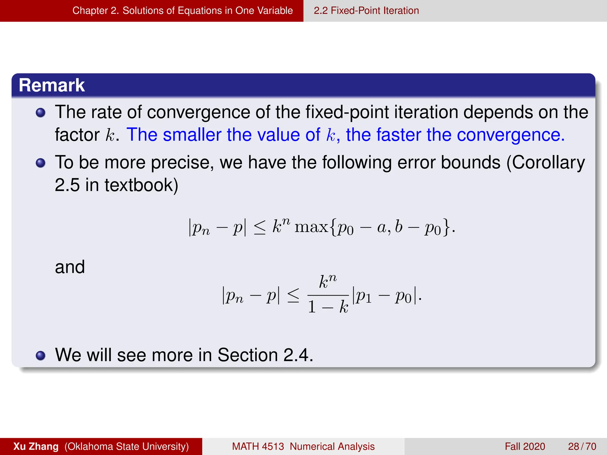
![Chapter 2. Solutions of Equations in One Variable 2.2 Fixed-Point Iteration
Proof (read if you like)
Since p ∈ [a, b], then
|pn − p| ≤ kn
|p0 − p| ≤ kn
max{p0 − a, b − p0}.
For n ≥ 1,
|pn+1 − pn| = |g(pn) − g(pn−1)| ≤ k|pn − pn−1| ≤ · · · ≤ kn
|p1 − p0|.
For m ≥ n ≥ 1,
|pm − pn| = |pm − pm−1 + pm−1 − · · · − pn+1 + pn+1 − pn|
≤ |pm − pm−1| + |pm1 − pm−2| + · · · + |pn+1 − pn|
≤ km−1
|p1 − p0| + km−2
|p1 − p0| + · · · kn
|p1 − p0|
≤ kn
|p1 − p0| 1 + k + k2
+ km−n−1
.
Xu Zhang (Oklahoma State University) MATH 4513 Numerical Analysis Fall 2020 29 / 70](https://image.slidesharecdn.com/na-ch2-student-250312030552-a1f8b621/75/NA-Ch2-Student-pdf-numerical-computing-chapter-2-solution-29-2048.jpg)
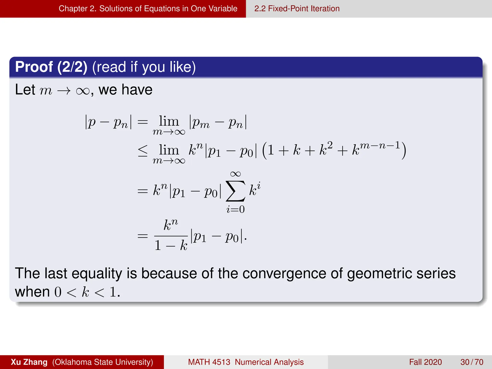
![Chapter 2. Solutions of Equations in One Variable 2.2 Fixed-Point Iteration
A revisit of the fixed-point schemes g1 to g5 in Example 2.9.
For g1(x) = x − x3 − 4x2 + 10, we know that
g1(1) = 6, and g2(2) = −12,
so g1 does not map [1, 2] into itself. Moreover,
|g0
1(x)| = |1 − 3x2
− 8x| 1, for all x ∈ [1, 2].
There is no reason to expect convergence.
For g2(x) =
r
10
x
− 4x, it does not map [1, 2] into [1, 2]. Also, there
is no interval containing the fixed point p ≈ 1.365 such that
|g0
2(x)| 1, because |g0
2(p)| ≈ 3.4 1. There is no reason to
expect it to converge.
Xu Zhang (Oklahoma State University) MATH 4513 Numerical Analysis Fall 2020 31 / 70](https://image.slidesharecdn.com/na-ch2-student-250312030552-a1f8b621/75/NA-Ch2-Student-pdf-numerical-computing-chapter-2-solution-31-2048.jpg)
![Chapter 2. Solutions of Equations in One Variable 2.2 Fixed-Point Iteration
A revisit of the fixed-point schemes g1 to g5 in Example 2.9.
For g3(x) =
1
2
√
10 − x3, we have
g0
3(x) = −
3
4
x2
(10 − x3
)−1/2
0, on [1, 2]
so g3 is strictly decreasing on [1, 2]. If we start with p0 = 1.5, it suffices to
consider the interval [1, 1.5]. Also note that
1 1.28 ≈ g3(1.5) ≤ g3(x) ≤ g3(1) = 1.5,
so g3 maps [1, 1.5] into itself. Moreover, it is also true that
|g0
3(x)| ≤ g0
3(1.5) ≈ 0.66,
on the interval [1, 1.5], so Theorem 2.10 guarantees its convergence.
(k ≈ 0.66)
Xu Zhang (Oklahoma State University) MATH 4513 Numerical Analysis Fall 2020 32 / 70](https://image.slidesharecdn.com/na-ch2-student-250312030552-a1f8b621/75/NA-Ch2-Student-pdf-numerical-computing-chapter-2-solution-32-2048.jpg)
![Chapter 2. Solutions of Equations in One Variable 2.2 Fixed-Point Iteration
A revisit of the fixed-point schemes g1 to g5 in Example 2.9.
For g4(x) =
r
10
4 + x
, it maps [1, 2] into itself. Moreover,
|g0
4(x)| ≤ |
√
10
2
(4+x)−3/2
| ≤
√
10
2
·5−3/2
=
1
5
√
2
0.15, for all x ∈ [1, 2].
So g4 converges much more rapidly than g3 (k ≈ 0.15).
For g5(x) = x −
x3
+ 4x2
− 10
3x2 + 8x
, it converges much more rapidly than
other choices. This choice of the g5(x) is in fact the Newton’s Method,
and we will see where this choice came from and why it is so effective in
the next section.
Xu Zhang (Oklahoma State University) MATH 4513 Numerical Analysis Fall 2020 33 / 70](https://image.slidesharecdn.com/na-ch2-student-250312030552-a1f8b621/75/NA-Ch2-Student-pdf-numerical-computing-chapter-2-solution-33-2048.jpg)
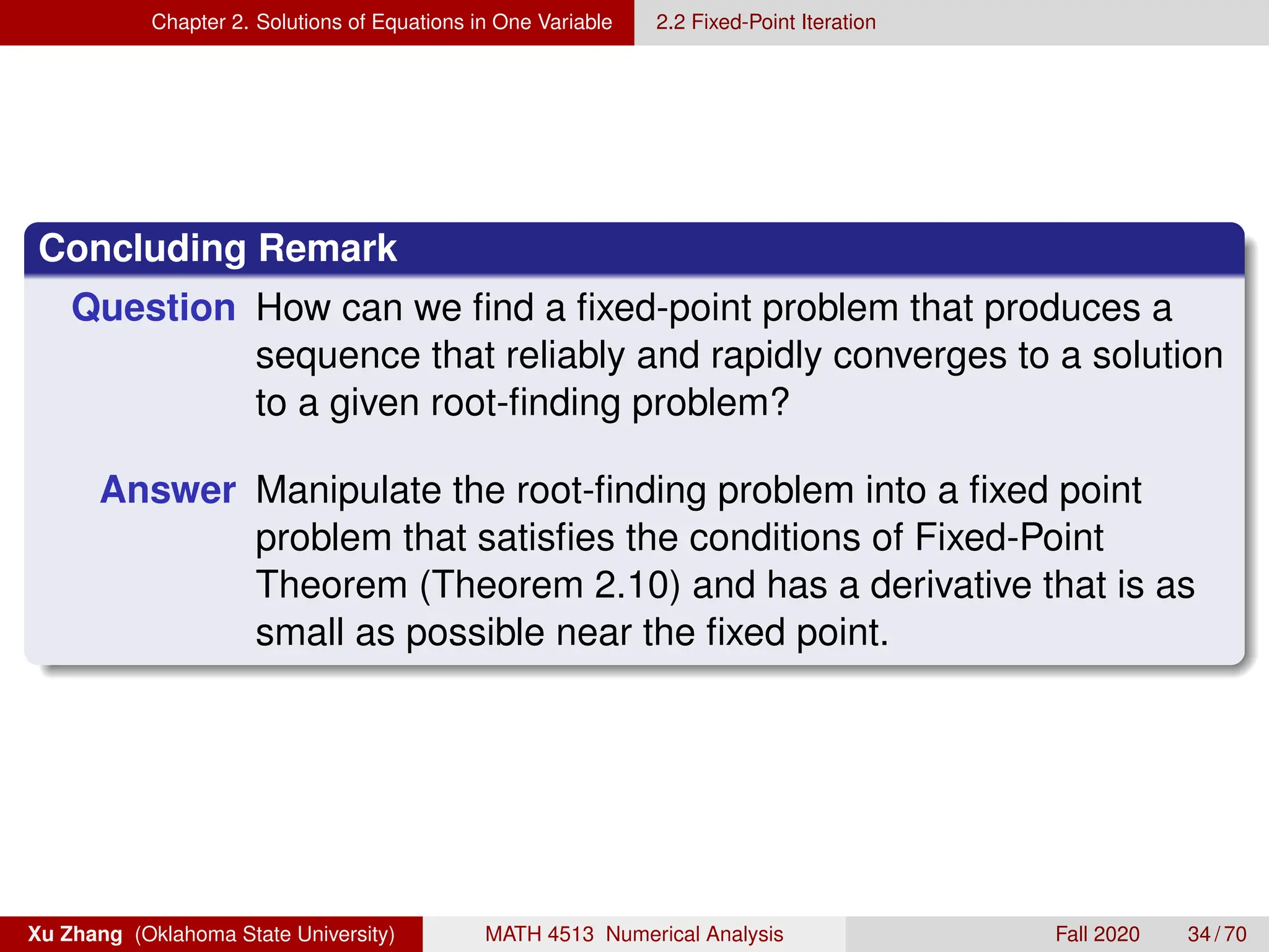
![Chapter 2. Solutions of Equations in One Variable 2.3 Newton’s Method and Its Extensions
2.3 Newton’s Method and Its Extensions
In this section, we introduce one of the most powerful and well-known
numerical methods for root-finding problems, namely Newton’s method
(or Newton-Raphson method).
Suppose f ∈ C2
[a, b]. Let p0 ∈ (a, b) be an approximation to a root p such
that f0
(p0) 6= 0. Assume that |p − p0| is small. By Taylor expansion,
f(p) = f(p0) + (p − p0)f0
(p0) +
(p − p0)2
2
f00
(ξ)
where ξ is between p0 and p.
Since f(p) = 0,
0 = f(p0) + (p − p0)f0
(p0) +
(p − p0)2
2
f00
(ξ)
Since p − p0 is small, we drop the high-order term involving (p − p0)2
,
0 ≈ f(p0) + (p − p0)f0
(p0) =⇒ p ≈ p0 −
f(p0)
f0(p0)
≡ p1.
Xu Zhang (Oklahoma State University) MATH 4513 Numerical Analysis Fall 2020 35 / 70](https://image.slidesharecdn.com/na-ch2-student-250312030552-a1f8b621/75/NA-Ch2-Student-pdf-numerical-computing-chapter-2-solution-35-2048.jpg)
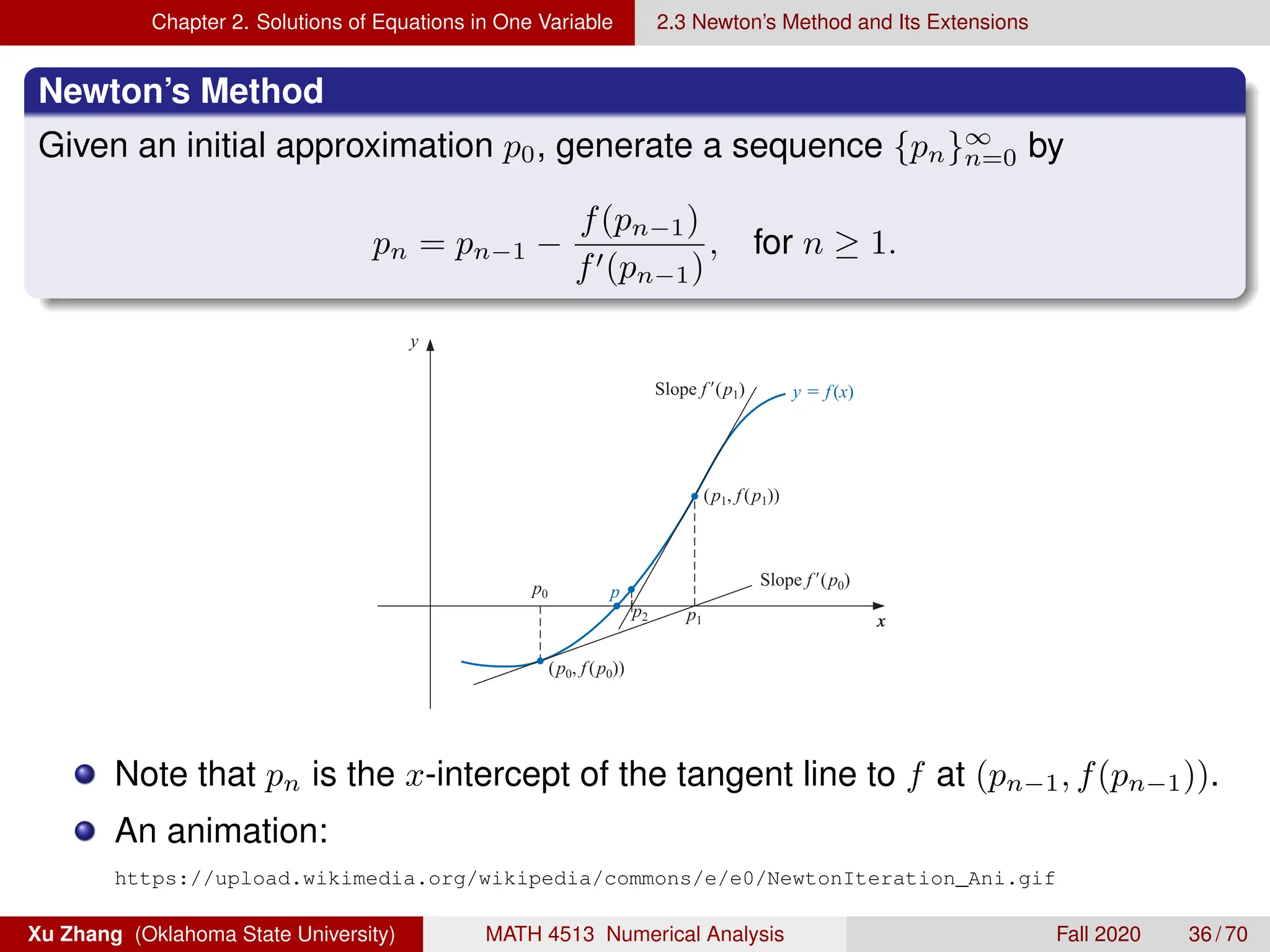
![Chapter 2. Solutions of Equations in One Variable 2.3 Newton’s Method and Its Extensions
To program the Newton’s method, the inputs should contain f, p0, tol,
maxit, as used in the fixed-point methods.
In addition, we also need to include the derivative f0
as an input.
Matlab Code of Newton’s Method
9/3/18 11:41 PM /Users/xuzhang/Dropbox/Teachin.../newton.m 1 of 1
function [p,flag] = newton(fun,Dfun,p0,tol,maxIt)
n = 0; flag = 0; % Initializaiton
disp('-----------------------------------')
disp('Newton Method')
disp('-----------------------------------')
disp(' n p_n f(p_n)')
disp('-----------------------------------')
formatSpec = '%2d %.10f % .10f n';
fprintf(formatSpec,[n,p0,fun(p0)])
while n=maxIt
p = p0 - fun(p0)/Dfun(p0);
if abs(p-p0) tol
flag = 1; break;
else
n = n+1; p0 = p;
end
fprintf(formatSpec,[n,p,fun(p)])
end
Xu Zhang (Oklahoma State University) MATH 4513 Numerical Analysis Fall 2020 37 / 70](https://image.slidesharecdn.com/na-ch2-student-250312030552-a1f8b621/75/NA-Ch2-Student-pdf-numerical-computing-chapter-2-solution-37-2048.jpg)
![Chapter 2. Solutions of Equations in One Variable 2.3 Newton’s Method and Its Extensions
Example 11.
Let f(x) = cos(x) − x. Approximate a root of f using (i) the fixed-point
method with g(x) = cos(x) and (ii) Newton’s method.
Solution (1/3)
(i). Using the fixed-point function g(x) = cos(x), we can start the
fixed-point iteration with p0 = π/4.
g( pn−1) = pn−1 −
f ( pn−1)
f ( pn−1)
, for n ≥ 1. (2.11)
In fact, this is the functional iteration technique that was used to give the rapid convergence
we saw in column (e) of Table 2.2 in Section 2.2.
It is clear from Equation (2.7) that Newton’s method cannot be continued if f ( pn−1) =
0 for some n. In fact, we will see that the method is most effective when f is bounded away
from zero near p.
Example 1 Consider the function f (x) = cos x−x = 0. Approximate a root of f using (a) a fixed-point
method, and (b) Newton’s Method
Solution (a) A solution to this root-finding problem is also a solution to the fixed-point
problem x = cos x, and the graph in Figure 2.9 implies that a single fixed-point p lies in
[0, π/2].
Figure 2.9
y
x
y x
y cos x
1
1
e in the
on is in
degrees. This
ase unless
Xu Zhang (Oklahoma State University) MATH 4513 Numerical Analysis Fall 2020 38 / 70](https://image.slidesharecdn.com/na-ch2-student-250312030552-a1f8b621/75/NA-Ch2-Student-pdf-numerical-computing-chapter-2-solution-38-2048.jpg)
![Chapter 2. Solutions of Equations in One Variable 2.3 Newton’s Method and Its Extensions
Solution (2/3)
(ii). To apply Newton’s method, we calculate f0(x) = − sin(x) − 1. We
again start with p0 = π/4.
A MATLAB driver file for this example
9/2/19 11:23 AM /Users/xuzhang/Dropbox/Teachi.../ex2_3_1.m
% Example 2.3.1 in the Textbook
fun = @(x) cos(x)-x; % Function f(x)
Dfun = @(x) -sin(x)-1; % Derivative of f(x)
funF = @(x) cos(x); % Function for fixed point iteration
tol = 1E-10;
maxIt = 20;
%% Fixed-Point Iteration
p0 = pi/4;
[pF,flagF] = fixedpoint(funF,p0,tol,maxIt);
disp(' ')
%% Newton Method
p0 = pi/4;
[p,flag] = newton(fun,Dfun,p0,tol,maxIt);
disp(' ')
Xu Zhang (Oklahoma State University) MATH 4513 Numerical Analysis Fall 2020 39 / 70](https://image.slidesharecdn.com/na-ch2-student-250312030552-a1f8b621/75/NA-Ch2-Student-pdf-numerical-computing-chapter-2-solution-39-2048.jpg)
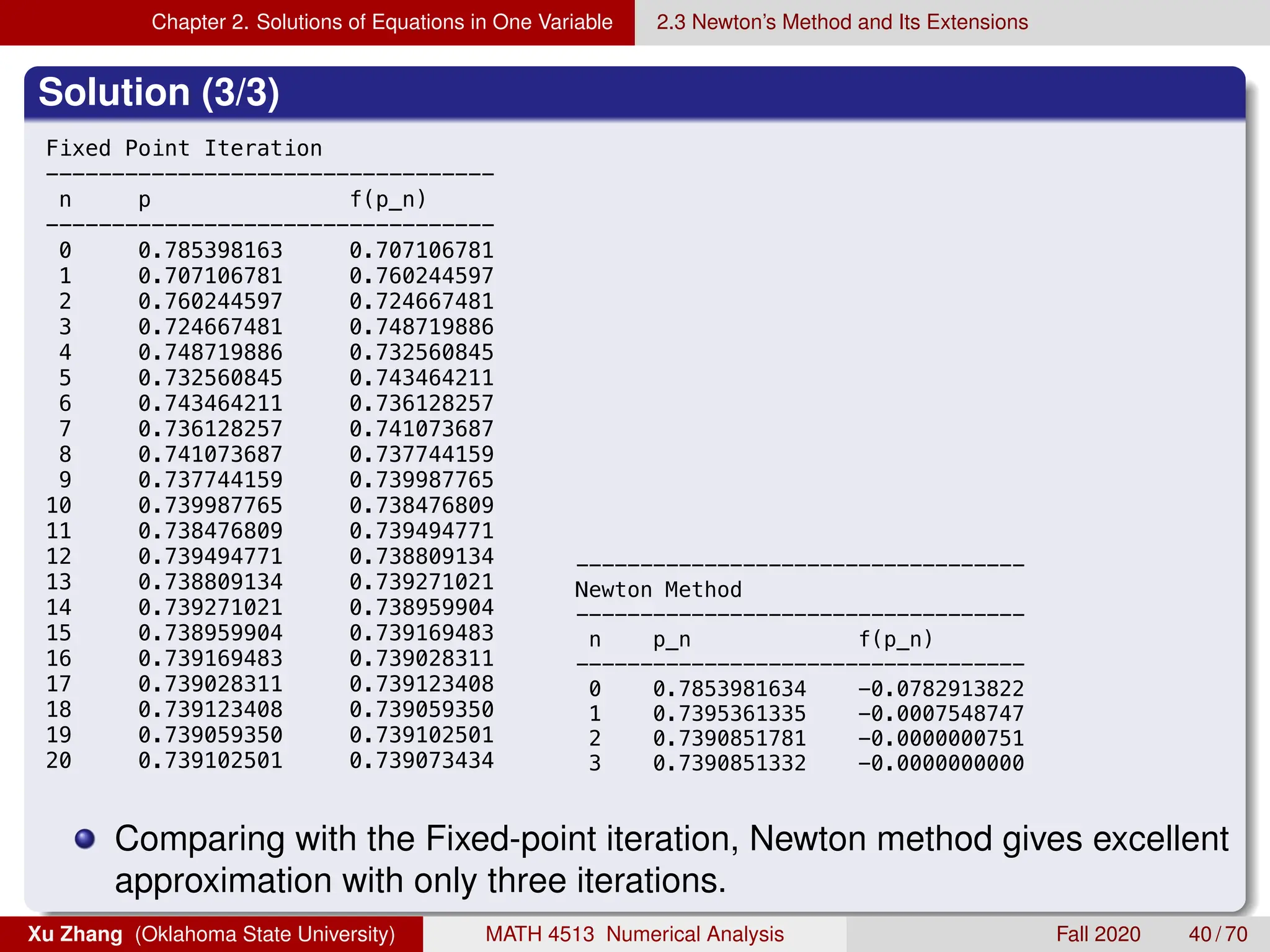
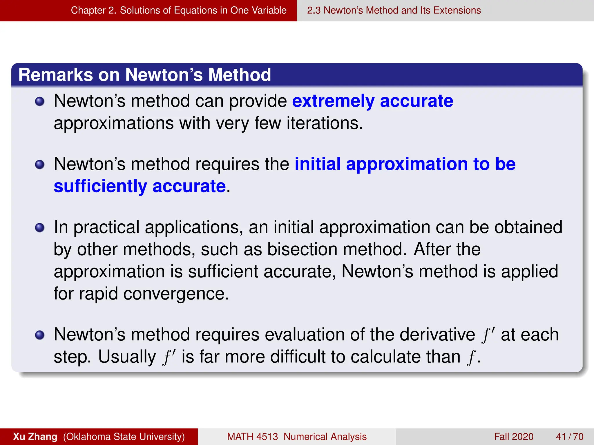
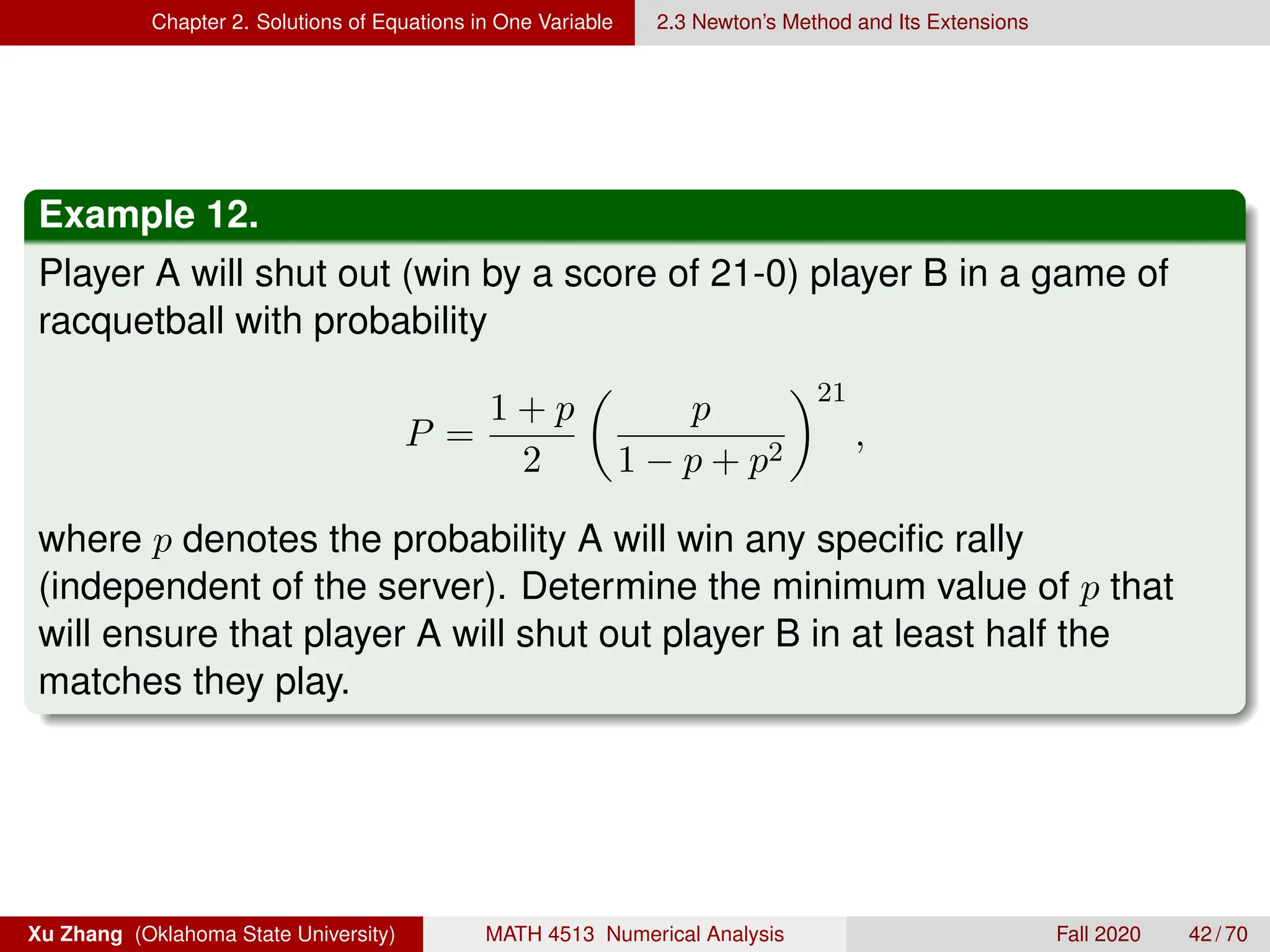
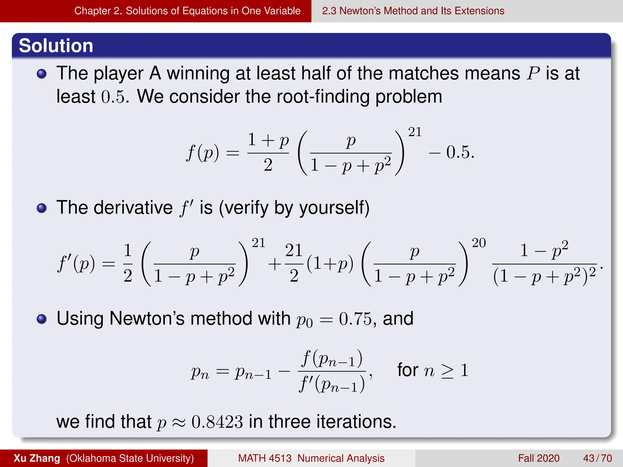
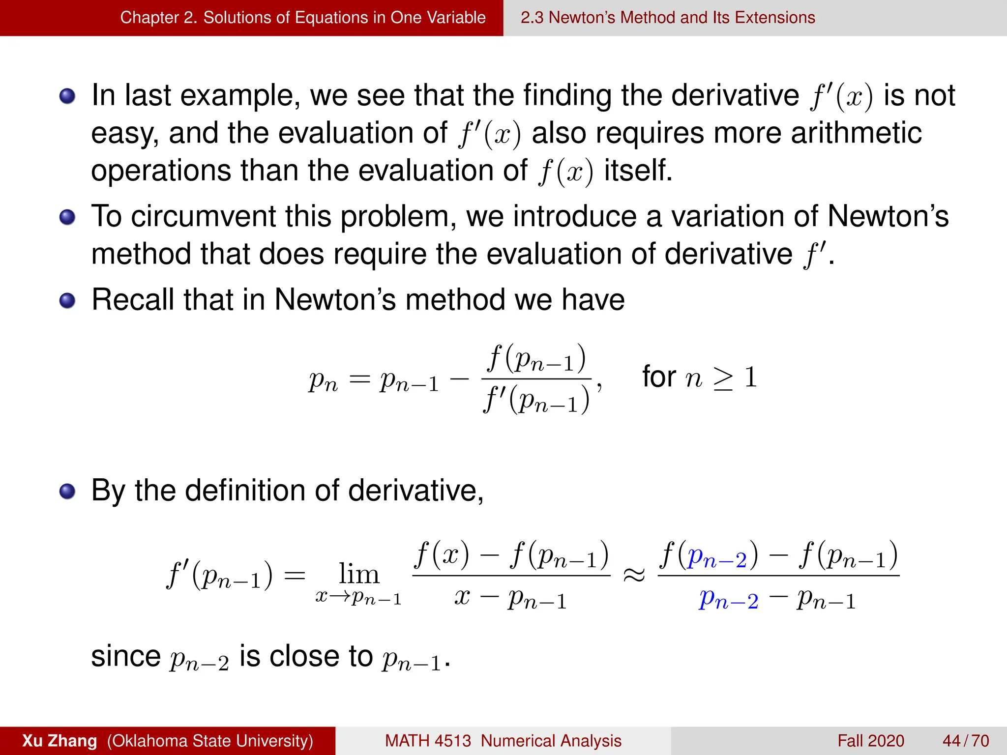
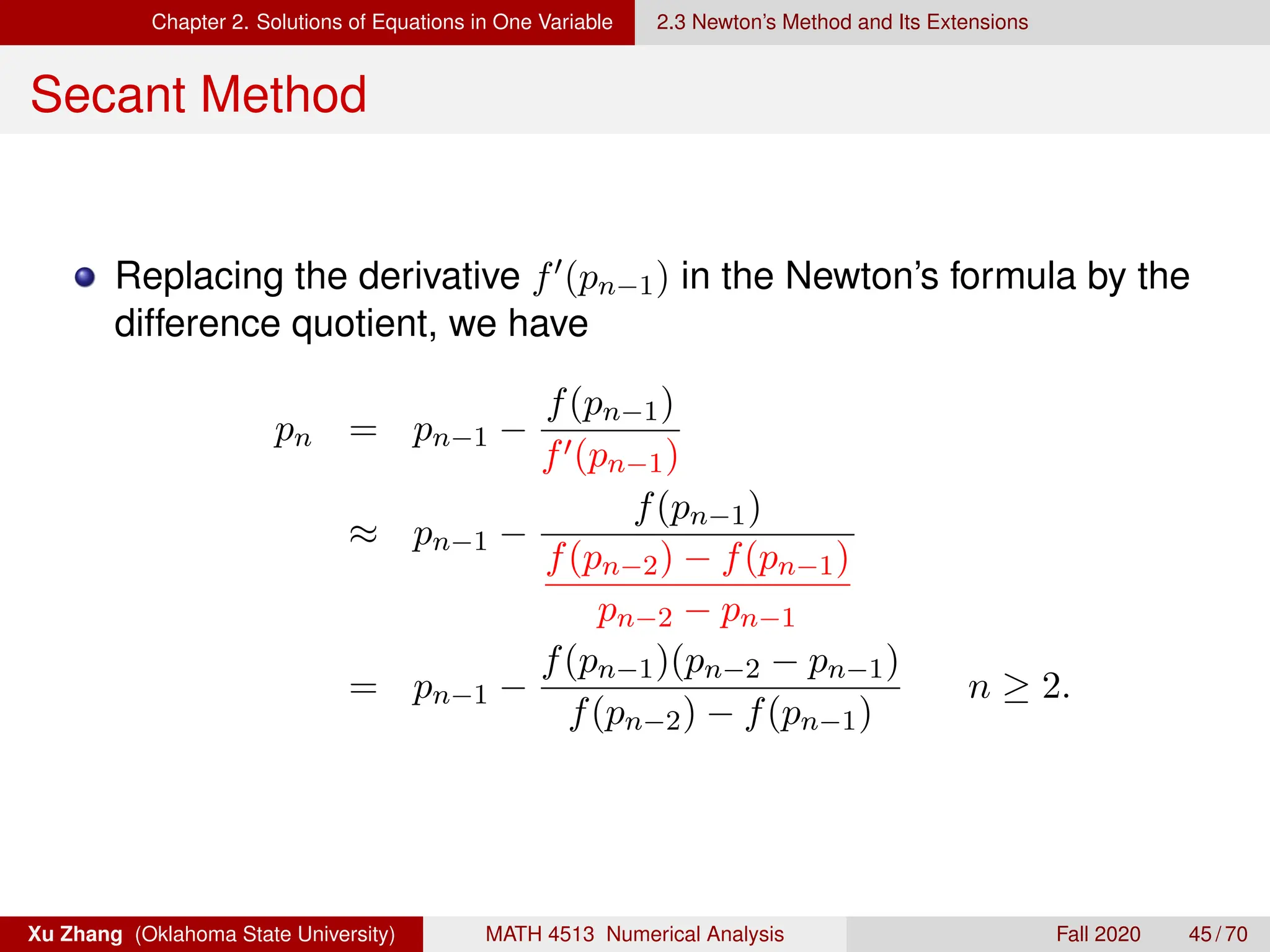
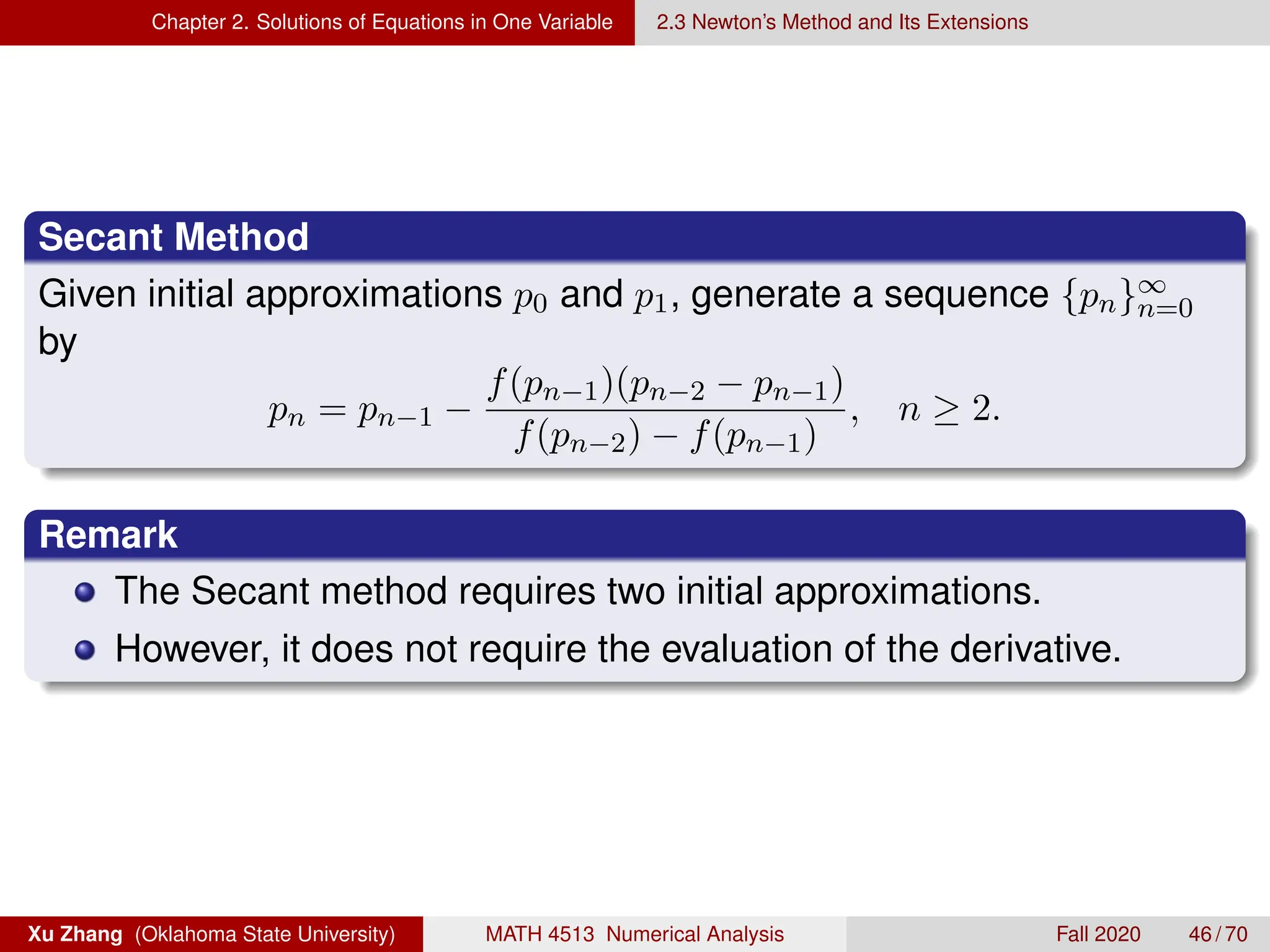
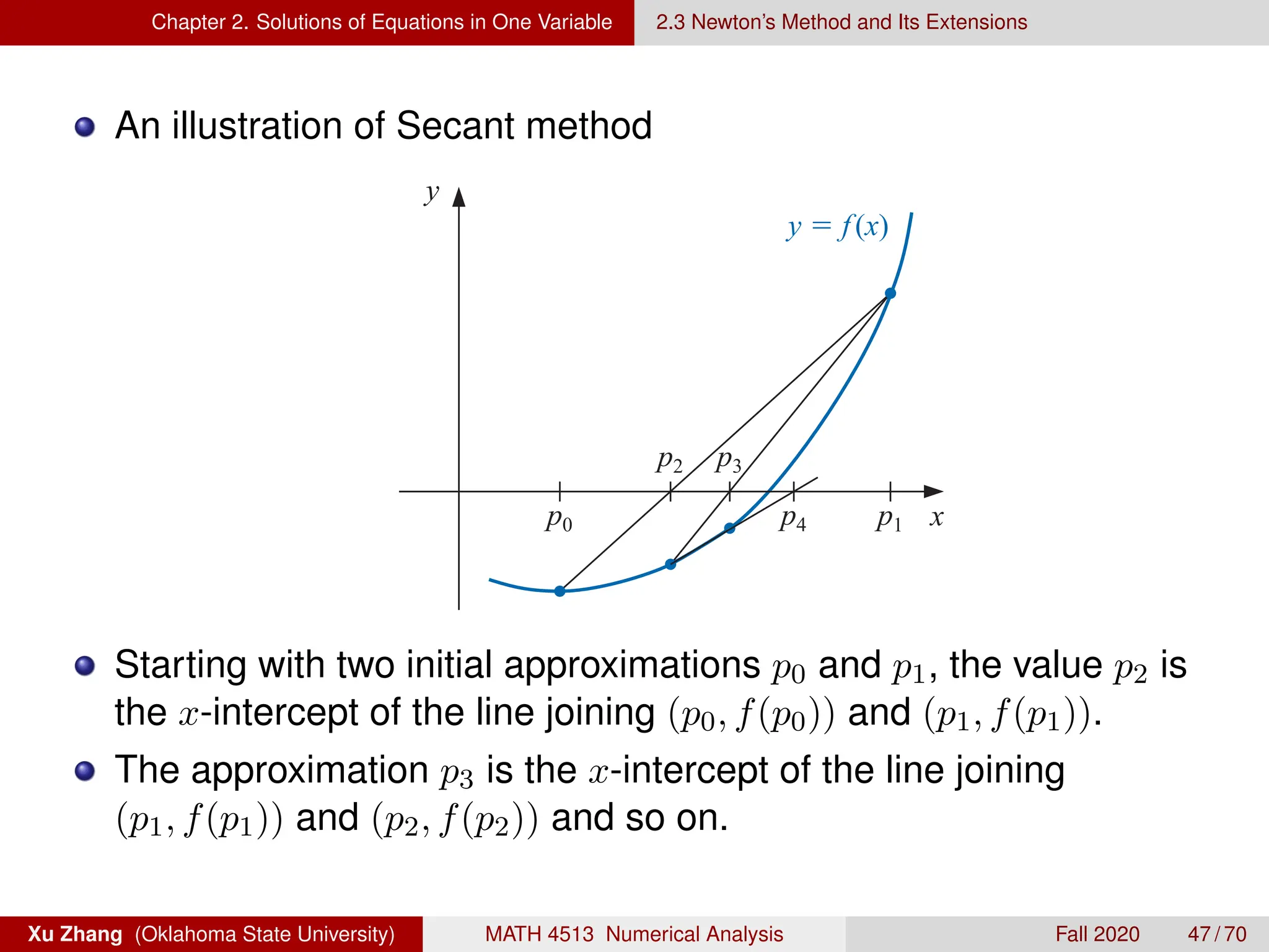
![Chapter 2. Solutions of Equations in One Variable 2.3 Newton’s Method and Its Extensions
Matlab Code of Secant Method
9/4/18 12:36 AM /Users/xuzhang/Dropbox/Teachin..
function [p,flag] = secant(fun,p0,p1,tol,maxIt)
n = 1; flag = 0; % Initializaiton
q0 = fun(p0); q1 = fun(p1);
disp('-----------------------------------')
disp('Secant Method')
disp('-----------------------------------')
disp(' n p_n f(p_n)')
disp('-----------------------------------')
formatSpec = '%2d %.10f % .10f n';
fprintf(formatSpec,[n-1,p0,fun(p0)])
fprintf(formatSpec,[n,p1,fun(p1)])
while n=maxIt
p = p1 - q1*(p1-p0)/(q1-q0);
if abs(p-p0) tol
flag = 1; break;
else
n = n+1;
p0 = p1; q0 = q1; p1 = p; q1 = fun(p);
end
fprintf(formatSpec,[n,p,fun(p)])
end
Xu Zhang (Oklahoma State University) MATH 4513 Numerical Analysis Fall 2020 48 / 70](https://image.slidesharecdn.com/na-ch2-student-250312030552-a1f8b621/75/NA-Ch2-Student-pdf-numerical-computing-chapter-2-solution-48-2048.jpg)
![Chapter 2. Solutions of Equations in One Variable 2.3 Newton’s Method and Its Extensions
Example 13.
Use the Secant method for find a solution to x = cos(x), and compare
with the approximation with those given from Newton’s method.
Solution (1/2)
Write a MATLAB driver file
9/4/18 12:37 AM /Users/xuzhang/Dropbox/Teachi...
% Example 2.3.2 in the Textbook
fun = @(x) cos(x)-x;
Dfun = @(x) -sin(x)-1;
tol = 1E-10;
maxIt = 40;
%% Newton
p0 = pi/4;
[pN,flagN] = newton(fun,Dfun,p0,tol,maxIt);
disp(' ')
%% Secant
p0 = 0.5; p1 = pi/4;
[pS,flagS] = secant(fun,p0,p1,tol,maxIt);
disp(' ')
Xu Zhang (Oklahoma State University) MATH 4513 Numerical Analysis Fall 2020 49 / 70](https://image.slidesharecdn.com/na-ch2-student-250312030552-a1f8b621/75/NA-Ch2-Student-pdf-numerical-computing-chapter-2-solution-49-2048.jpg)
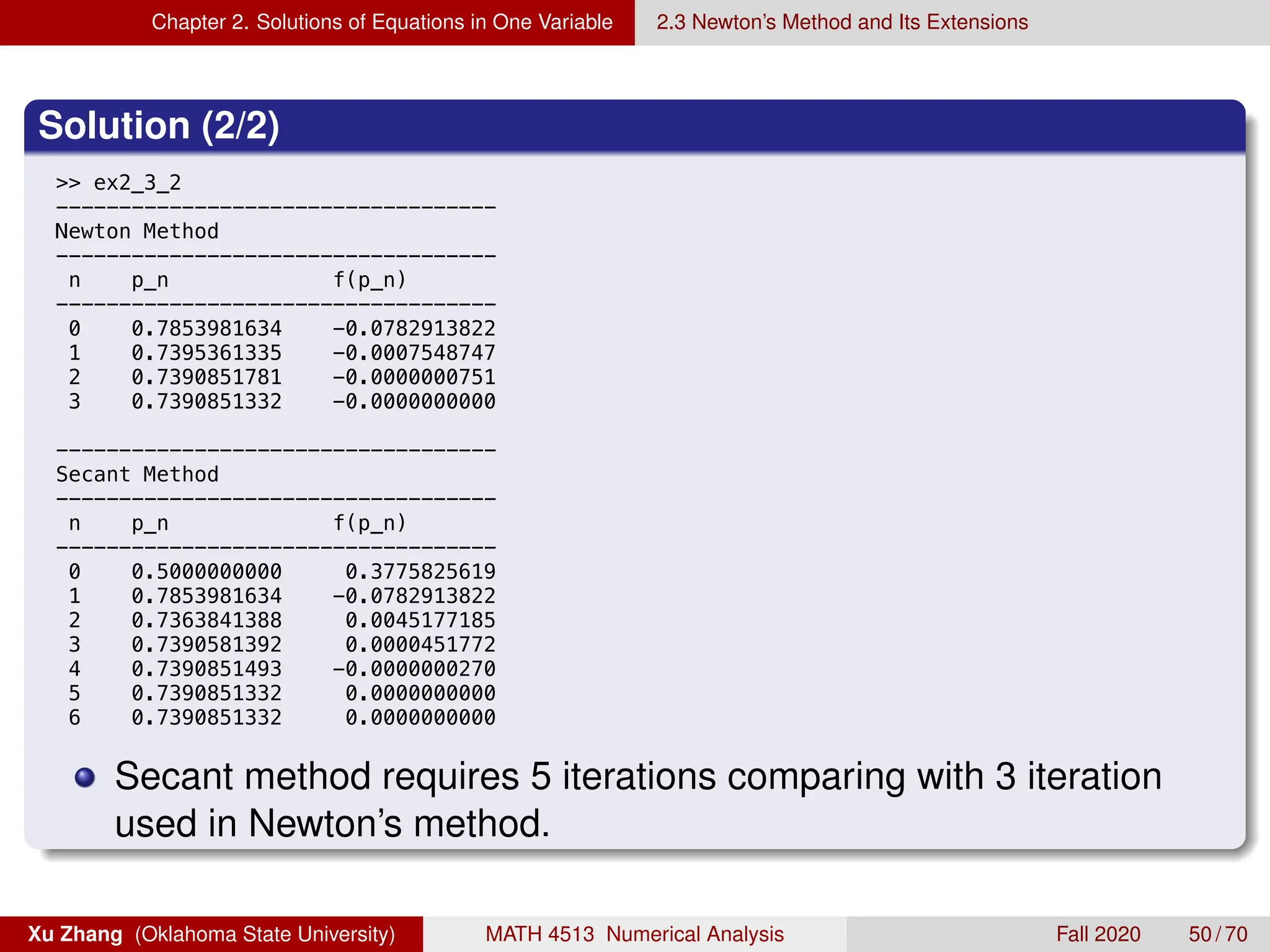
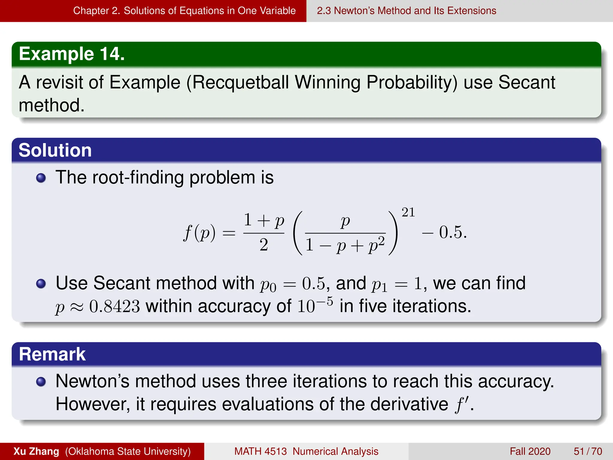
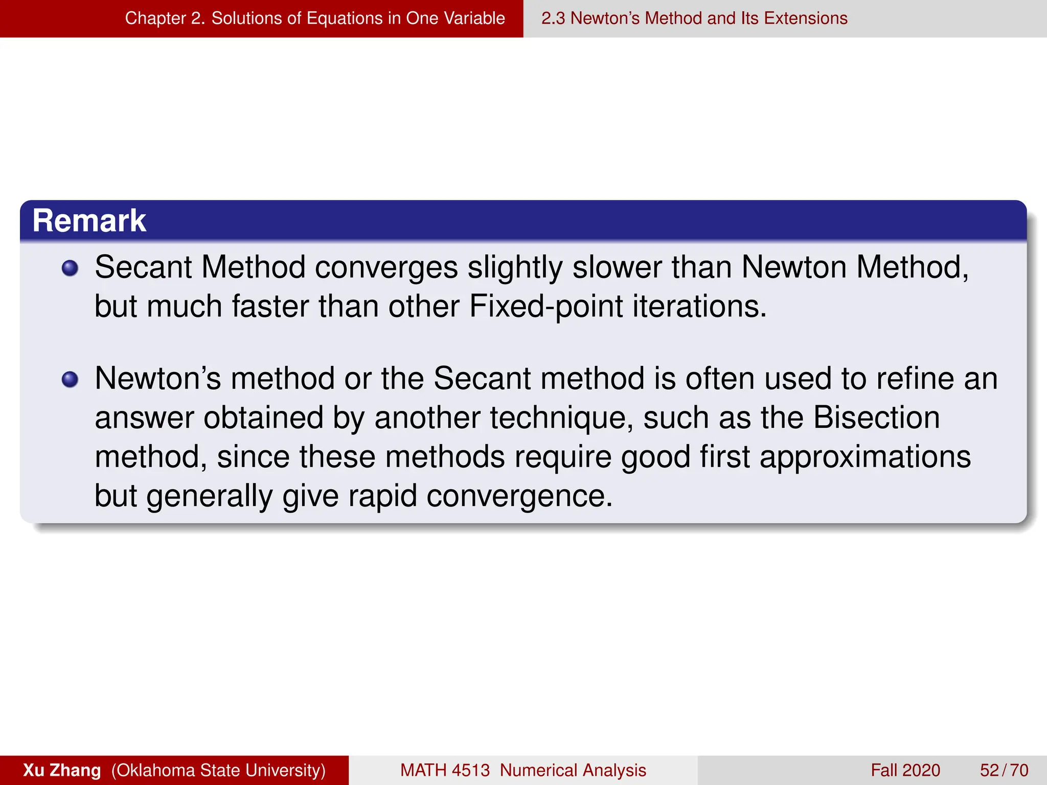
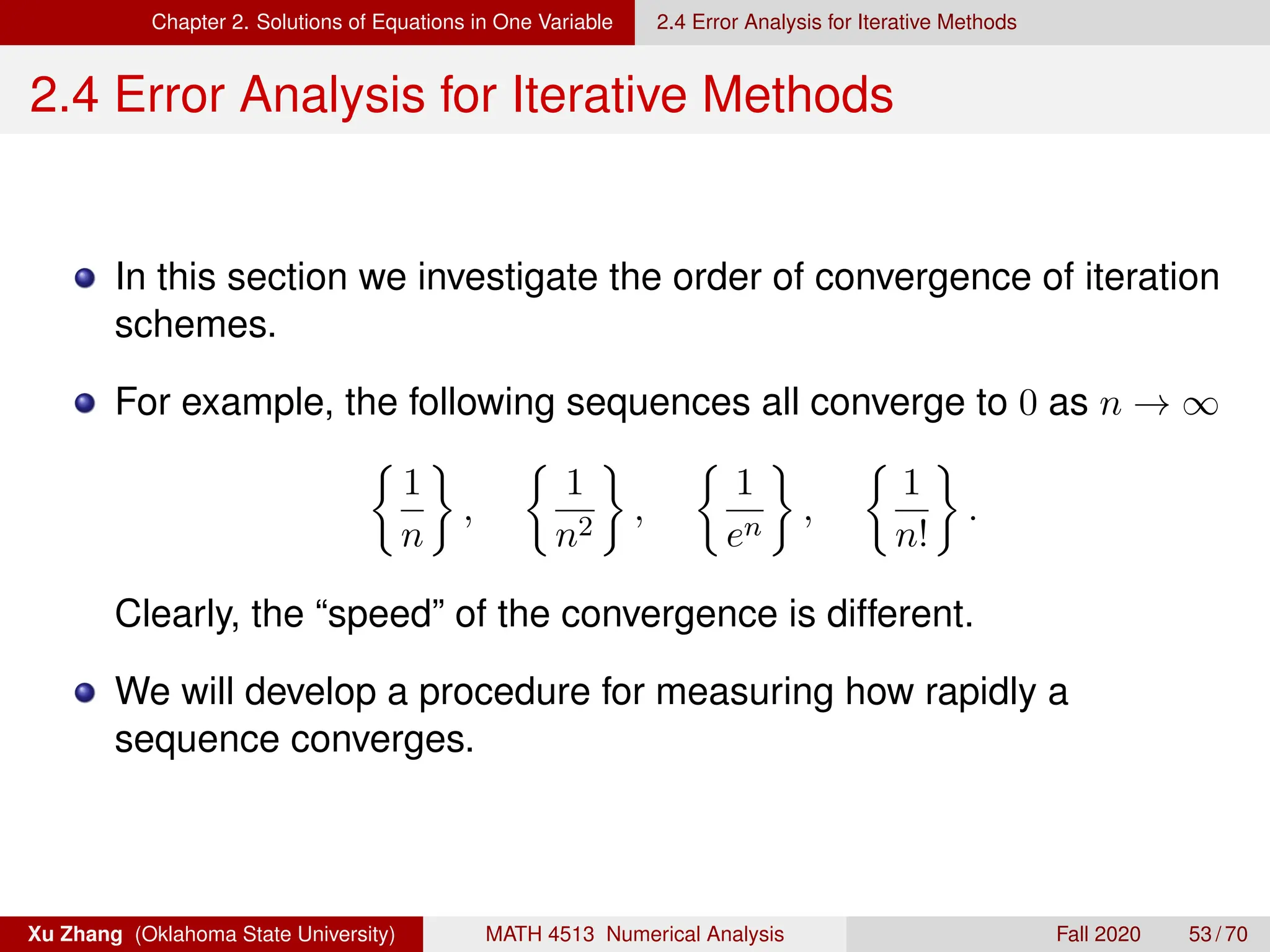
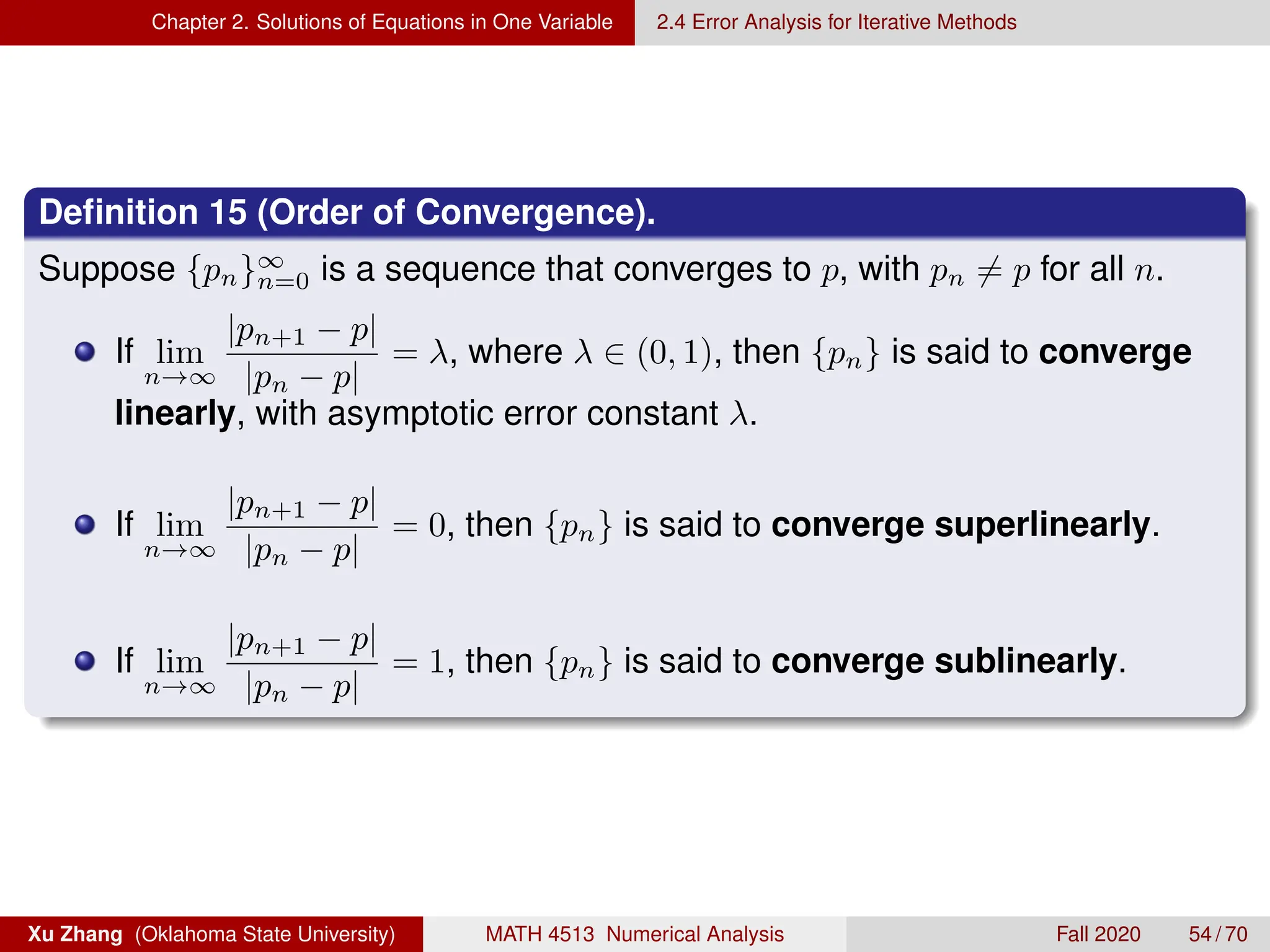
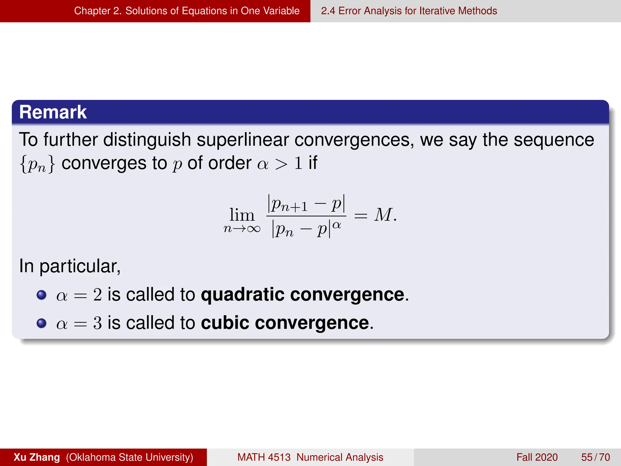
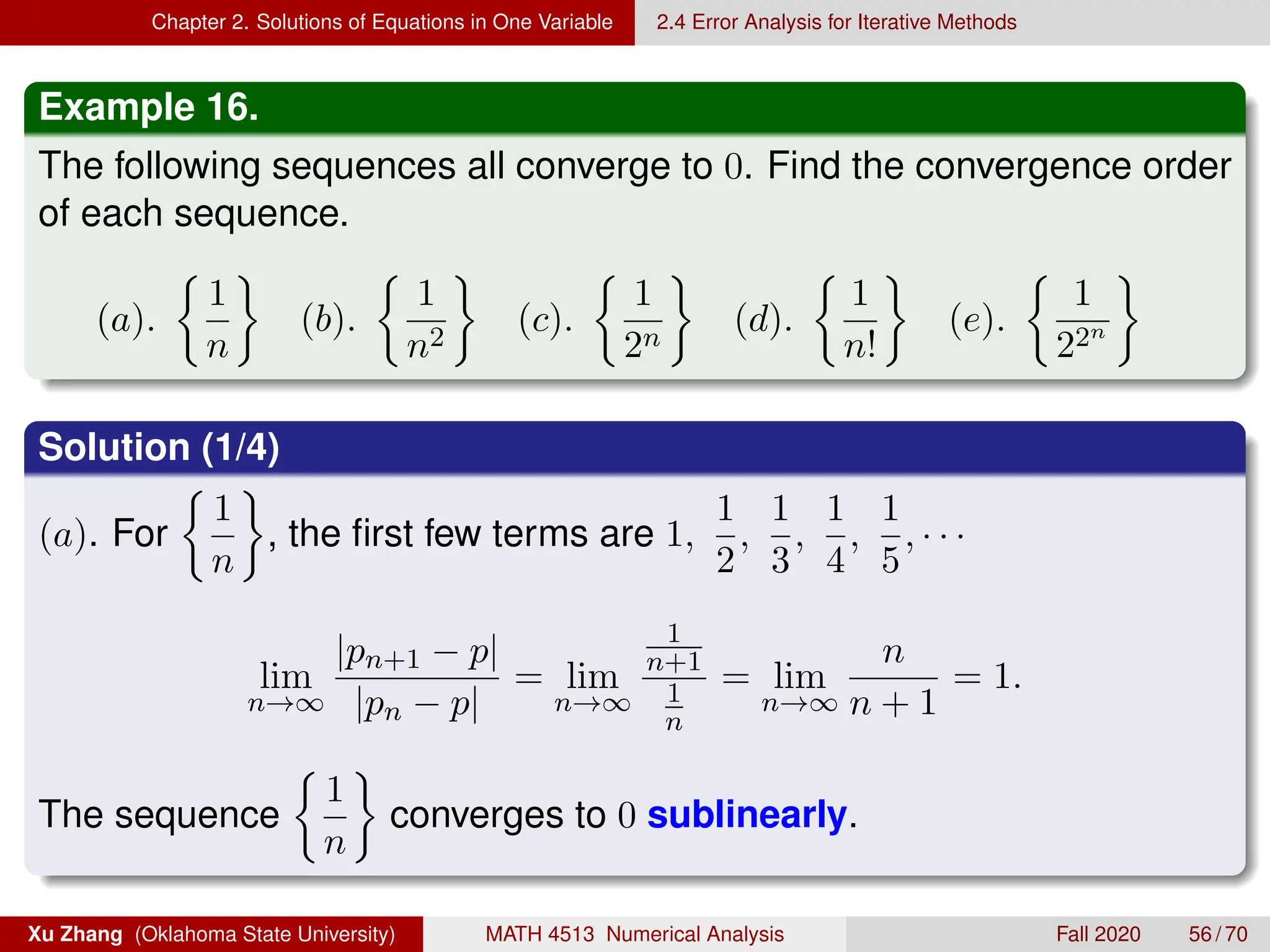
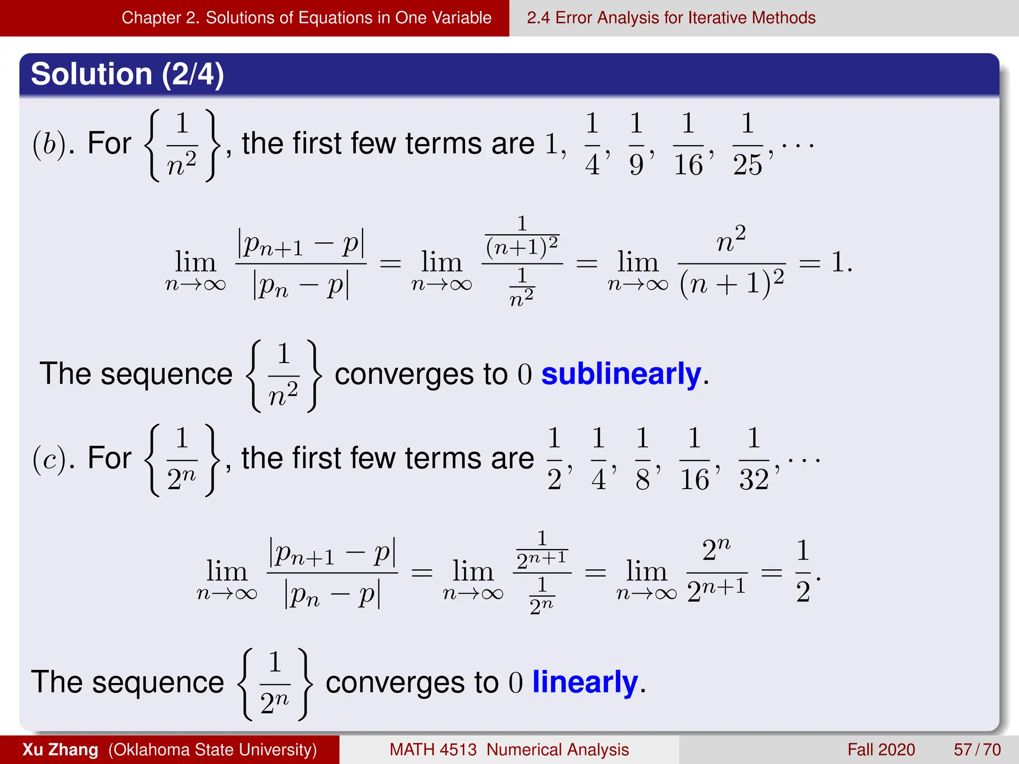
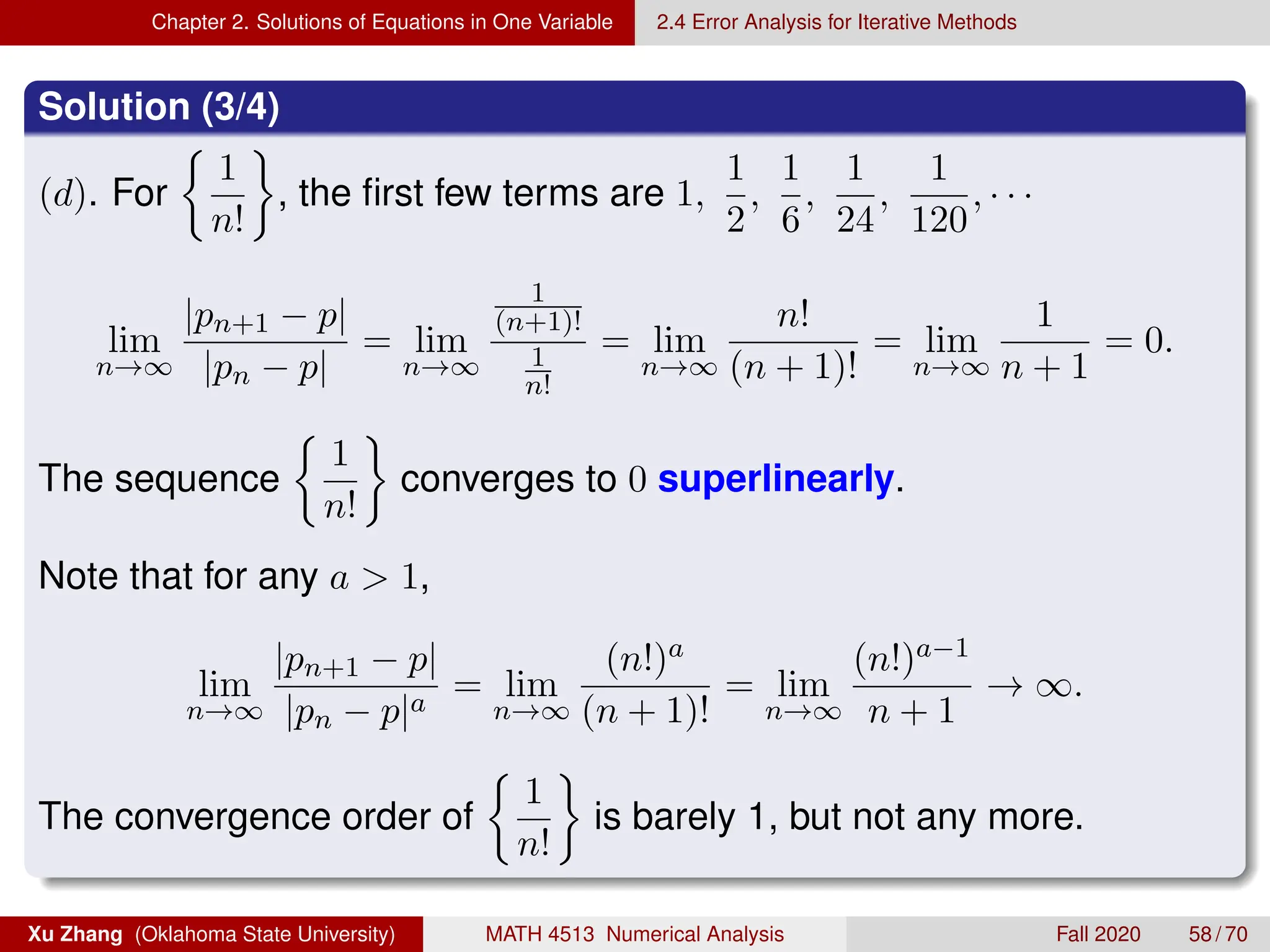
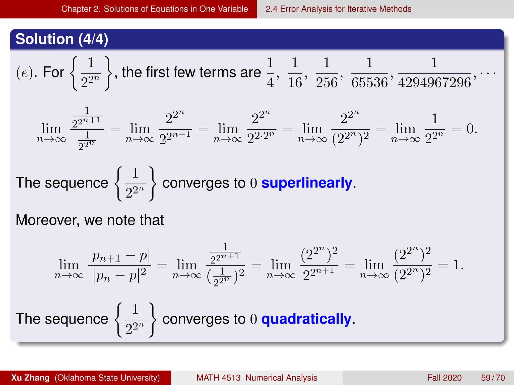
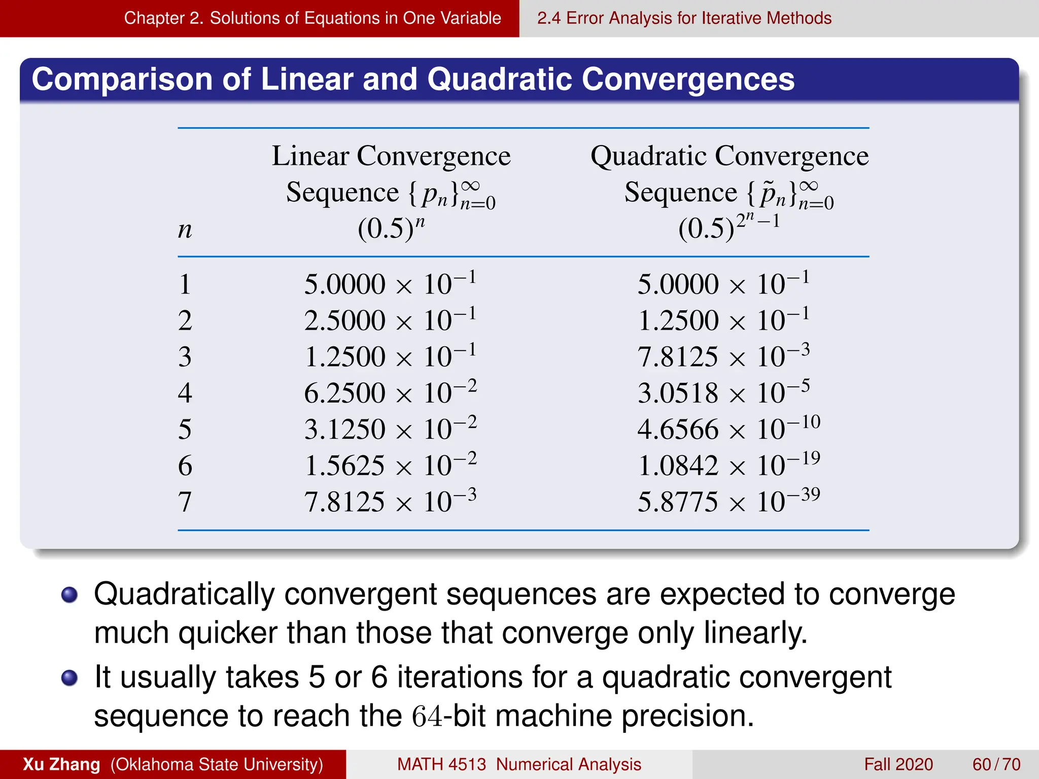
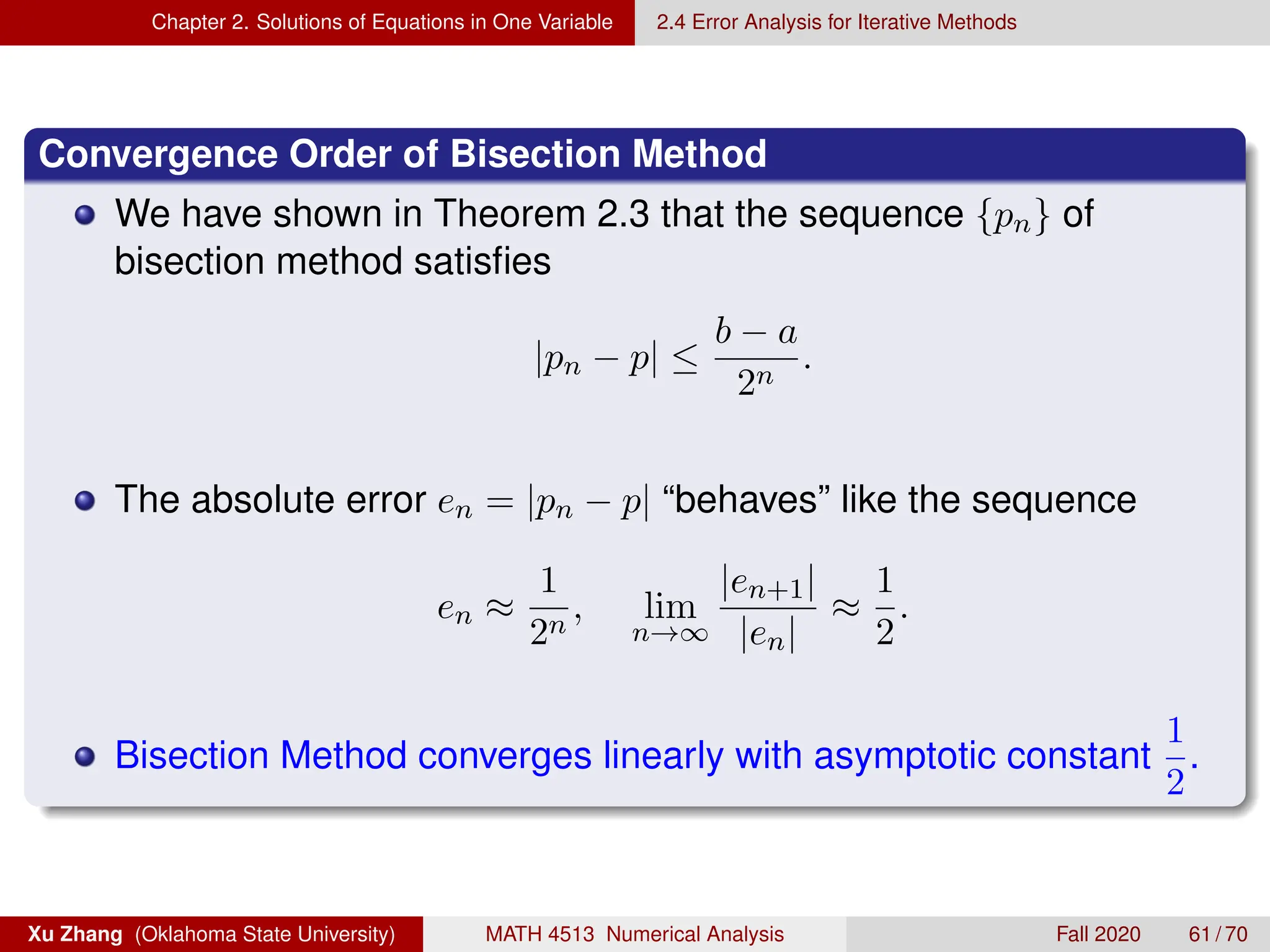
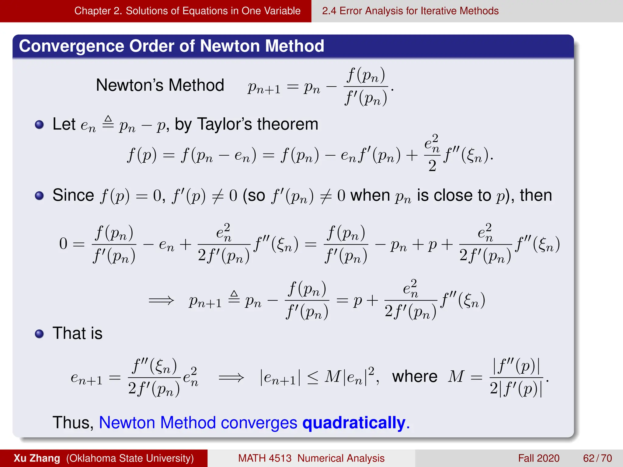
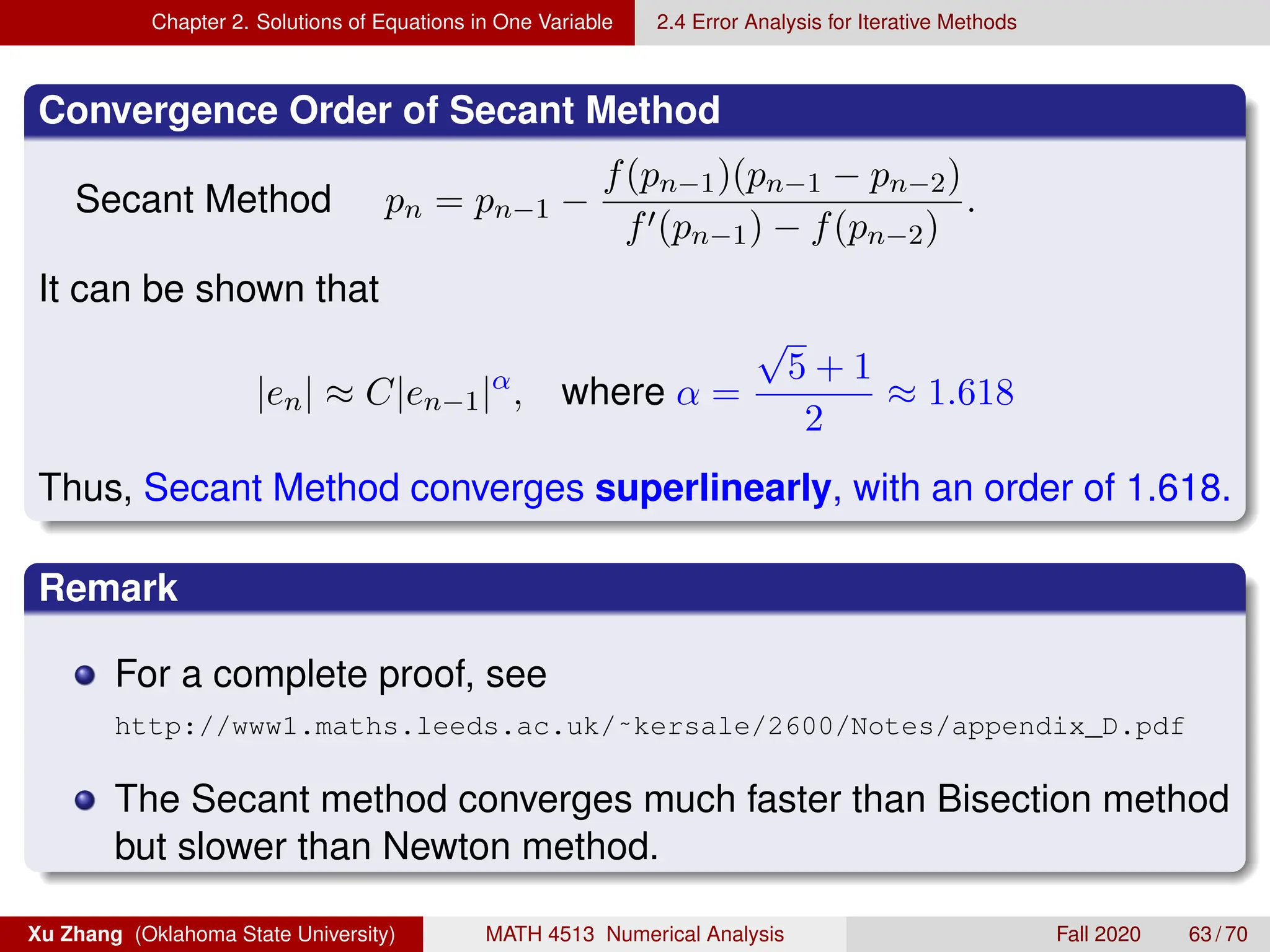
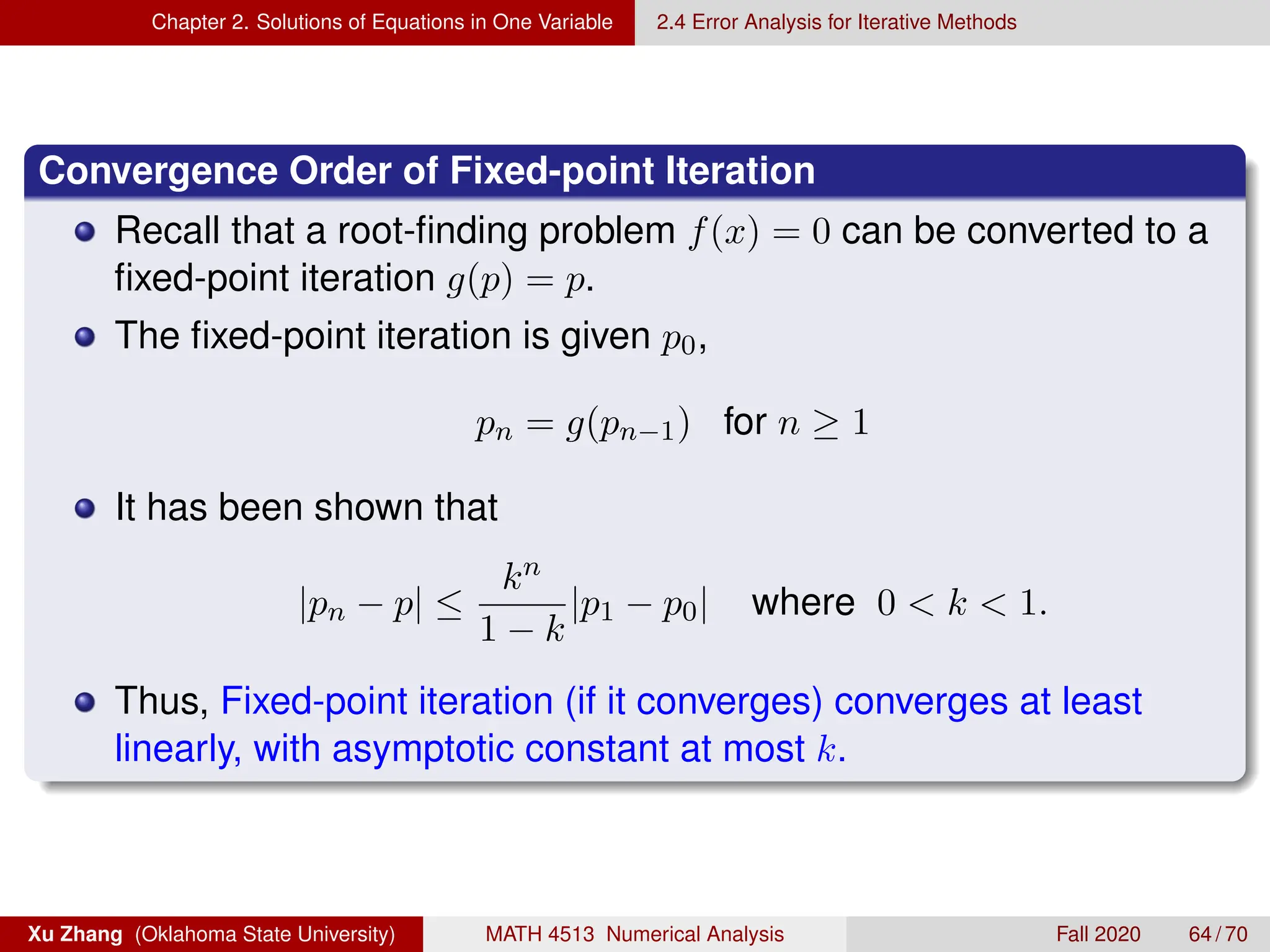
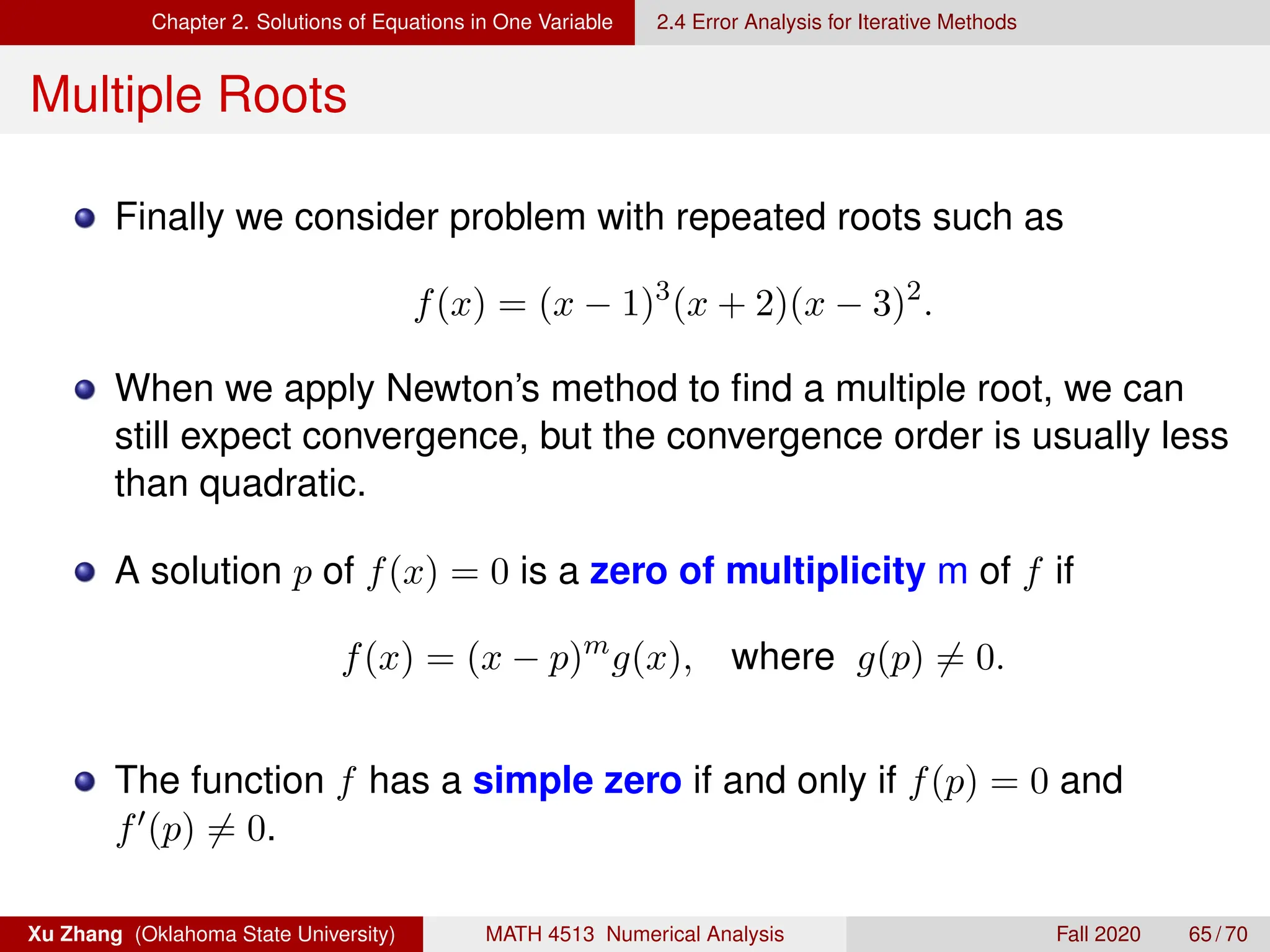
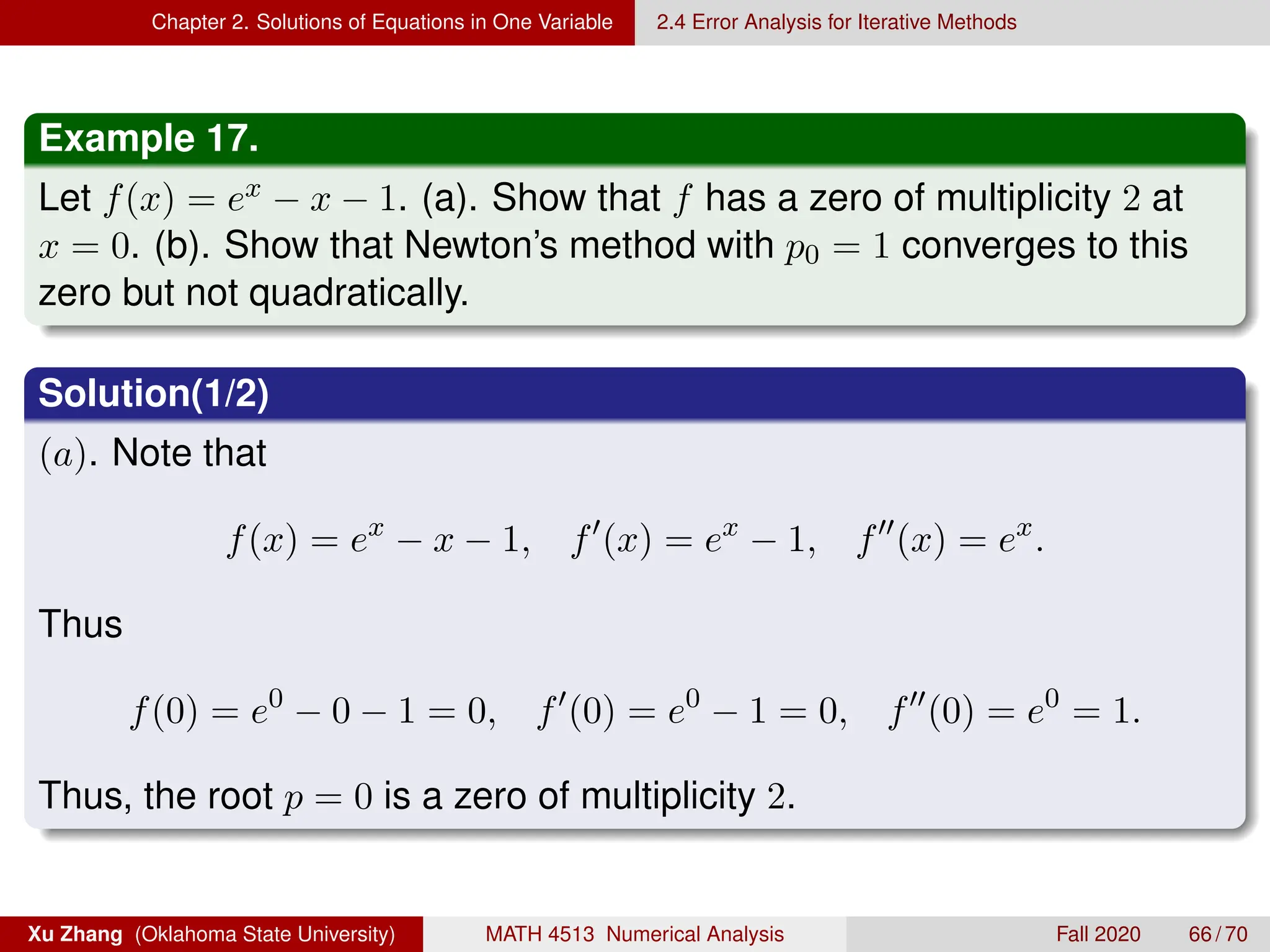
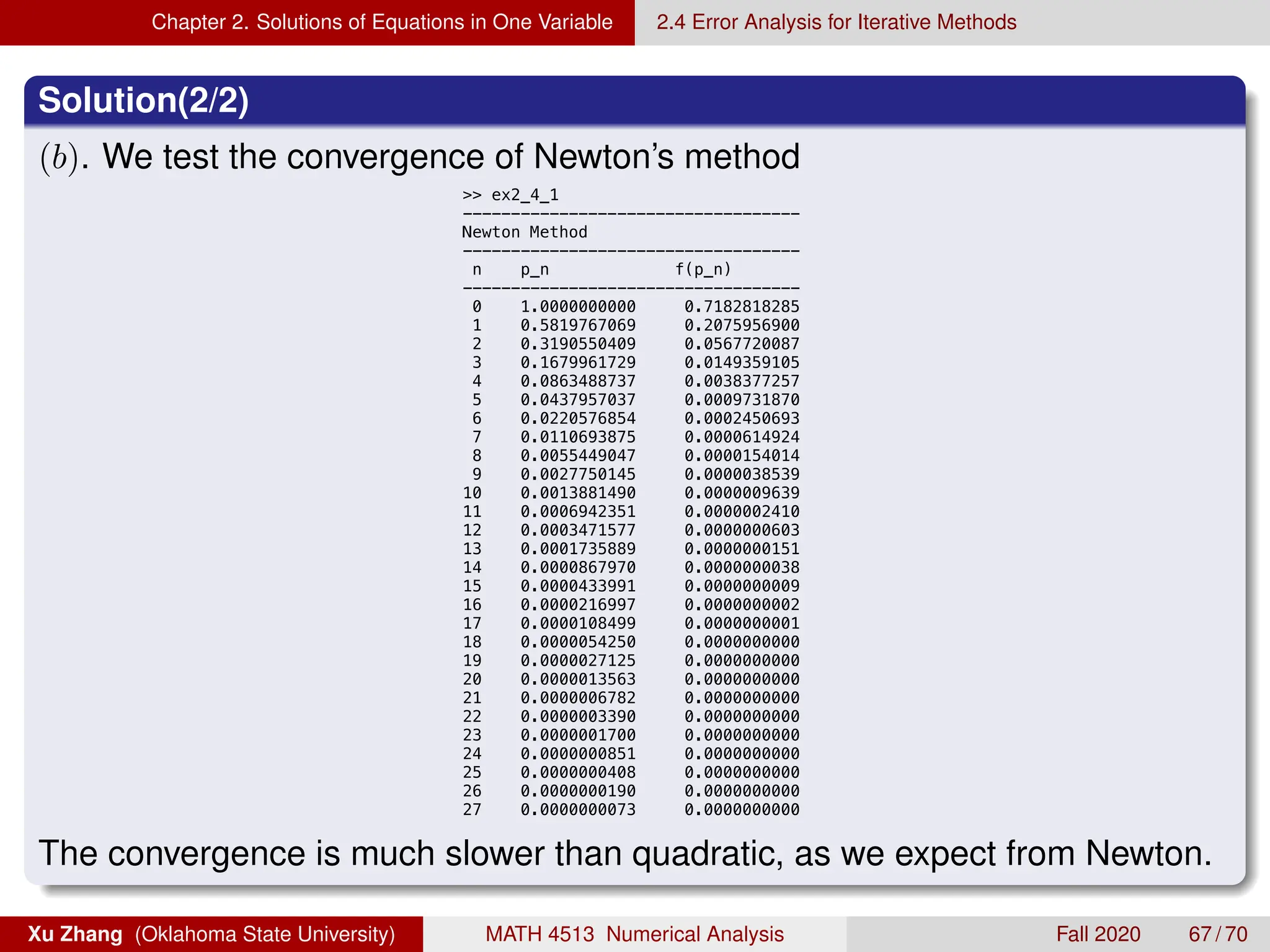
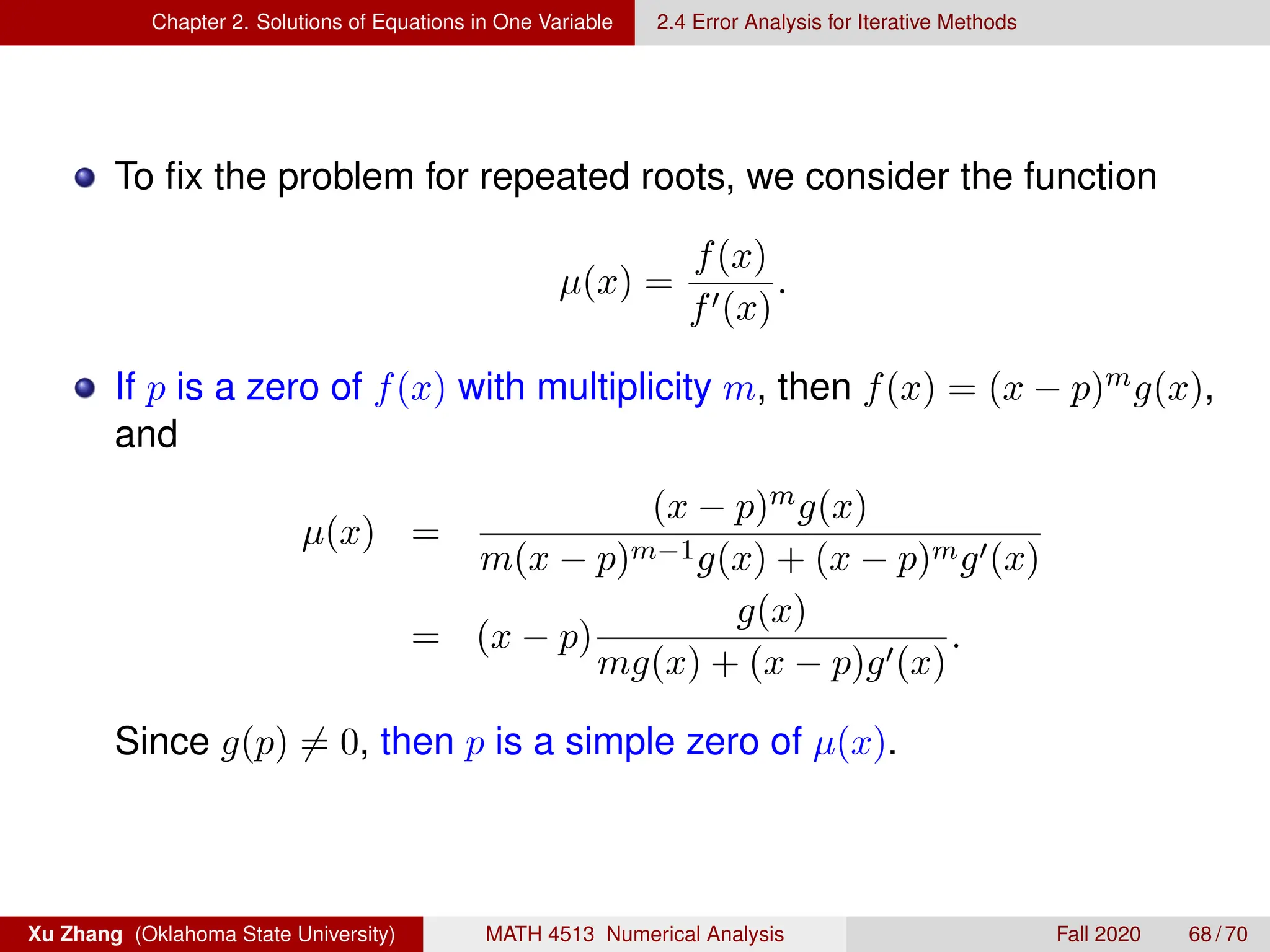
![Chapter 2. Solutions of Equations in One Variable 2.4 Error Analysis for Iterative Methods
Now to find the zero p, we apply Newton’s method to µ(x),
g(x) = x −
µ(x)
µ0(x)
= x −
f(x)/f0(x)
[f0(x)]2 − f(x)f00(x)
[f0(x)]2
= x −
f(x)f0(x)
[f0(x)]2 − f(x)f00(x)
.
Modified Newton’s Method (for multiple roots)
Given an initial approximation p0, generate a sequence {pn}∞
n=0 by
pn = pn−1 −
f(pn−1)f0(pn−1)
[f0(pn−1)]2 − f(pn−1)f00(pn−1)
, for n ≥ 1.
Note: The modified Newton’ method requires the second-order
derivative f00(x).
Xu Zhang (Oklahoma State University) MATH 4513 Numerical Analysis Fall 2020 69 / 70](https://image.slidesharecdn.com/na-ch2-student-250312030552-a1f8b621/75/NA-Ch2-Student-pdf-numerical-computing-chapter-2-solution-69-2048.jpg)
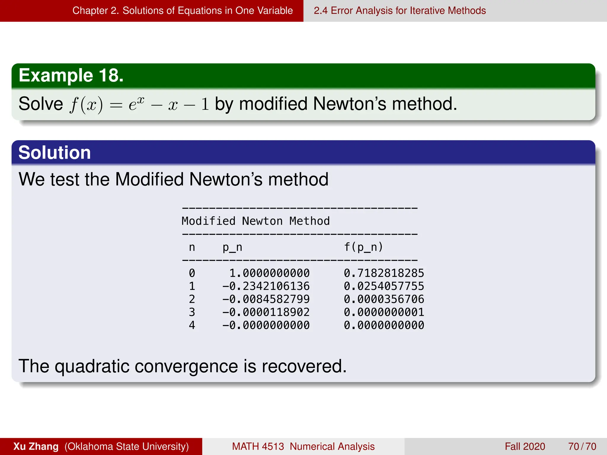


![Chapter 2. Solutions of Equations in One Variable 2.1 The Bisection Method
Section 2.1 The Bisection Method
Starting from this section, we study the most basic mathematics
problem: root-finding problem
f(x) = 0.
The first numerical method, based on the Intermediate Value
Theorem (IVT), is called the Bisection Method.
Suppose that f(x) is continuous on [a, b]. f(a) and f(b) have
opposite sign. By IVT, there exists a number p ∈ (a, b) such that
f(p) = 0. That is, f(x) has a root in (a, b).
Idea of Bisection Method: repeatedly halve the subinterval of
[a, b], and at each step, locating the half containing the root.
Xu Zhang (Oklahoma State University) MATH 4513 Numerical Analysis Fall 2020 3 / 70](https://crownmelresort.com/image.slidesharecdn.com/na-ch2-student-250312030552-a1f8b621/75/NA-Ch2-Student-pdf-numerical-computing-chapter-2-solution-3-2048.jpg)
![Chapter 2. Solutions of Equations in One Variable 2.1 The Bisection Method
Set a1 ← a, b1 ← b. Calculate the midpoint p1 ← a1+b1
2 .
2.1 The Bisection Method 49
Figure 2.1
x
y
f(a)
f(p2)
f (p1)
f(b)
y f(x)
a a1 b b1
p p1
p2
p3
a1 b1
p1
p2
a2 b2
p3
a3 b3
ALGORITHM
2.1
Bisection
To find a solution to f (x) = 0 given the continuous function f on the interval [a, b], where
f (a) and f (b) have opposite signs:
INPUT endpoints a, b; tolerance TOL; maximum number of iterations N0.
If f(p1) = 0, then p ← p1, done.
If f(p1) 6= 0, then f(p1) has the same sign as either f(a) or f(b).
If f(p1) and f(a) have the same sign, then p ∈ (p1, b1).
Set a2 ← p1, and b2 ← b1.
If f(p1) and f(b) have the same sign, then p ∈ (a1, p1).
Set a2 ← a1, and b2 ← p1.
Repeat the process on [a2, b2].
Xu Zhang (Oklahoma State University) MATH 4513 Numerical Analysis Fall 2020 4 / 70](https://crownmelresort.com/image.slidesharecdn.com/na-ch2-student-250312030552-a1f8b621/75/NA-Ch2-Student-pdf-numerical-computing-chapter-2-solution-4-2048.jpg)
![Chapter 2. Solutions of Equations in One Variable 2.1 The Bisection Method
ALGORITHM – Bisection (Preliminary Version)
USAGE: to find a solution to f(x) = 0 on the interval [a, b].
p = bisect0 (f, a, b)
For n = 1, 2, 3, · · · , 20, do the following
Step 1 Set p = (a + b)/2;
Step 2 Calculate FA = f(a), FB = f(b), and FP = f(p).
Step 3 If FA · FP 0, set a = p
If FB · FP 0, set b = p.
Go back to Step 1.
Remark
This above algorithm will perform 20 times bisection iterations. The
number 20 is artificial.
Xu Zhang (Oklahoma State University) MATH 4513 Numerical Analysis Fall 2020 5 / 70](https://crownmelresort.com/image.slidesharecdn.com/na-ch2-student-250312030552-a1f8b621/75/NA-Ch2-Student-pdf-numerical-computing-chapter-2-solution-5-2048.jpg)
![Chapter 2. Solutions of Equations in One Variable 2.1 The Bisection Method
Example 1.
Show that f(x) = x3 + 4x2 − 10 = 0 has a root in [1, 2] and use the
Bisection method to find the approximation root.
Solution.
Because f(1) = −5 and f(2) = 14, the IVT ensures that this
continuous function has a root in [1, 2].
To proceed with the Bisection method, we write a simple MATLAB
code.
Xu Zhang (Oklahoma State University) MATH 4513 Numerical Analysis Fall 2020 6 / 70](https://crownmelresort.com/image.slidesharecdn.com/na-ch2-student-250312030552-a1f8b621/75/NA-Ch2-Student-pdf-numerical-computing-chapter-2-solution-6-2048.jpg)

![Chapter 2. Solutions of Equations in One Variable 2.1 The Bisection Method
After 20 iterations, we obtain the solution p ≈ 1.365229606628418.
To display more information from the whole iteration process, we
modify the MATLAB subroutine file.
Matlab Code for Bisection (Preliminary Version with more outputs)
8/21/19 5:39 PM /Users/xuzhang/Dropbox/Teachi.../bisect1.m 1 of 1
function p = bisect1(fun,a,b)
% This is a preliminary version of Bisection Method
% This version displays intermediate outputs nicely
disp('Bisection Methods')
disp('-----------------------------------------------------------------')
disp(' n a_n b_n p_n f(p_n)')
disp('-----------------------------------------------------------------')
formatSpec = '%2d % .9f % .9f % .9f % .9f n';
for n = 1:20 % Set max number of iterations to be 20
p = (a+b)/2;
FA = fun(a);
FB = fun(b);
FP = fun(p);
fprintf(formatSpec,[n,a,b,p,fun(p)]) % Printing output
if FA*FP 0
a = p;
elseif FB*FP 0
b = p;
end
end
Xu Zhang (Oklahoma State University) MATH 4513 Numerical Analysis Fall 2020 8 / 70](https://crownmelresort.com/image.slidesharecdn.com/na-ch2-student-250312030552-a1f8b621/75/NA-Ch2-Student-pdf-numerical-computing-chapter-2-solution-8-2048.jpg)
![Chapter 2. Solutions of Equations in One Variable 2.1 The Bisection Method
Some Remarks on Bisection Method
To start, an interval [a, b] must be found with f(a) · f(b) 0.
Otherwise, there may be no solutions in that interval.
It is good to set a maximum iteration number “maxit”, in case the
the iteration enters an endless loop.
It is good to set a tolerance or stopping criteria to avoid
unnecessary computational effort, such as
1
bn − an
2
tol
2 |pn − pn+1| tol
3
|pn − pn+1|
|pn|
tol
4 |f(pn)| tol
Xu Zhang (Oklahoma State University) MATH 4513 Numerical Analysis Fall 2020 9 / 70](https://crownmelresort.com/image.slidesharecdn.com/na-ch2-student-250312030552-a1f8b621/75/NA-Ch2-Student-pdf-numerical-computing-chapter-2-solution-9-2048.jpg)
![Chapter 2. Solutions of Equations in One Variable 2.1 The Bisection Method
A more robust Matlab code for Bisection method
8/27/19 12:00 AM /Users/xuzhang/Dropbox/Teachi.../bisect.m 1 of 1
function [p,flag] = bisect(fun,a,b,tol,maxIt)
%% This is a more robust version of Bisection Method than bisect1.m
flag = 0; % Use a flag to tell if the output is reliable
if fun(a)*fun(b) 0 % Check f(a) and f(b) have different sign
error('f(a) and f(b) must have different signs');
end
disp('Bisection Methods')
disp('-----------------------------------------------------------------')
disp(' n a_n b_n p_n f(p_n)')
disp('-----------------------------------------------------------------')
formatSpec = '%2d % .9f % .9f % .9f % .9f n';
for n = 1:maxIt
p = (a+b)/2;
FA = fun(a);
FP = fun(p);
fprintf(formatSpec,[n,a,b,p,fun(p)]) % Printing output
if abs(FP) = 10^(-15) || (b-a)/2 tol
flag = 1;
break; % Break out the for loop.
else
if FA*FP 0
a = p;
else
b = p;
end
end
end
Xu Zhang (Oklahoma State University) MATH 4513 Numerical Analysis Fall 2020 10 / 70](https://crownmelresort.com/image.slidesharecdn.com/na-ch2-student-250312030552-a1f8b621/75/NA-Ch2-Student-pdf-numerical-computing-chapter-2-solution-10-2048.jpg)
![Chapter 2. Solutions of Equations in One Variable 2.1 The Bisection Method
Example 2.
Use Bisection method to find a root of f(x) = x3 + 4x2 − 10 = 0 in the
interval [1, 2] that is accurate to at least within 10−4.
Solution.
We write a Matlab driver file for this test problem
8/14/18 2:17 PM /Users/zhang/Dropbox/Teaching.../ex2_1_1.
% Example 2.1.1 in the Textbook
fun = @(x) x^3+4*x^2-10;
a = 1;
b = 2;
tol = 1E-4;
maxIt = 40;
[p,flag] = bisect(fun,a,b,tol,maxIt);
In this driver file, we
specify all five inputs: fun, a, b, tol, maxIt
call the Bisection method code bisect.m.
Xu Zhang (Oklahoma State University) MATH 4513 Numerical Analysis Fall 2020 11 / 70](https://crownmelresort.com/image.slidesharecdn.com/na-ch2-student-250312030552-a1f8b621/75/NA-Ch2-Student-pdf-numerical-computing-chapter-2-solution-11-2048.jpg)

![Chapter 2. Solutions of Equations in One Variable 2.1 The Bisection Method
Theorem 3 (Convergence of Bisection Method).
Suppose that f ∈ C[a, b] and f(a) · f(b) 0. The Bisection method
generates a sequence {pn}∞
n=1 approximating a zero p of f with
|pn − p| ≤
b − a
2n
, when n ≥ 1.
Proof.
For n ≥ 1, we have p ∈ (an, bn) and
bn − an =
1
2n−1
(b − a).
Since pn = 1
2(an + bn) for all n ≥ 1, then
|pn − p| ≤
1
2
(bn − an) =
b − a
2n
.
Xu Zhang (Oklahoma State University) MATH 4513 Numerical Analysis Fall 2020 13 / 70](https://crownmelresort.com/image.slidesharecdn.com/na-ch2-student-250312030552-a1f8b621/75/NA-Ch2-Student-pdf-numerical-computing-chapter-2-solution-13-2048.jpg)


![Chapter 2. Solutions of Equations in One Variable 2.2 Fixed-Point Iteration
Theorem 7 (Sufficient Conditions for Fixed Points).
(i) (Existence) If g ∈ C[a, b] and g(x) ∈ [a, b] for all x ∈ [a, b], then g
has at least one fixed point in [a, b].
(ii) (Uniqueness) If, in addition, g0(x) exists and satisfies
|g0
(x)| ≤ k 1, for all x ∈ (a, b),
for some positive constant k, there is exactly one fixed-point in [a, b].
x
3 2 2 3
3
The following theorem gives sufficient conditions for the existence and uniqueness of
a fixed point.
Theorem 2.3 (i) If g ∈ C[a, b] and g(x) ∈ [a, b] for all x ∈ [a, b], then g has at least one fixed
point in [a, b].
(ii) If, in addition, g (x) exists on (a, b) and a positive constant k 1 exists with
|g (x)| ≤ k, for all x ∈ (a, b),
then there is exactly one fixed point in [a, b]. (See Figure 2.4.)
Figure 2.4
y
x
y x
y g(x)
p g(p)
a p b
a
b
Proof
(i) If g(a) = a or g(b) = b, then g has a fixed point at an endpoint. If not, then
g(a) a and g(b) b. The function h(x) = g(x)−x is continuous on [a, b], with
Note: the proof of existence uses the Intermediate Value Theorem, and
the proof of uniqueness uses the Mean Value Theorem.
Xu Zhang (Oklahoma State University) MATH 4513 Numerical Analysis Fall 2020 17 / 70](https://crownmelresort.com/image.slidesharecdn.com/na-ch2-student-250312030552-a1f8b621/75/NA-Ch2-Student-pdf-numerical-computing-chapter-2-solution-17-2048.jpg)
![Chapter 2. Solutions of Equations in One Variable 2.2 Fixed-Point Iteration
Example 8.
Show that g(x) =
1
3
(x2
− 1) has a unique fixed-point on [−1, 1].
Proof (1/2)
(1. Existence). We show that g(x) has at least a fixed point p ∈ [−1, 1].
Taking the derivative,
g0
(x) =
2x
3
, only one critical point x = 0, g(0) = −
1
3
.
At endpoints, x = −1 and 1, we have g(−1) = 0, and g(1) = 0.
Then we have the global extreme values
min
x∈[−1,1]
g(x) = −
1
3
, and max
x∈[−1,1]
g(x) = 0.
Therefore, g(x) ∈ [−1
3 , 0] ⊂ [−1, 1]. By the first part of Theorem 2.7, the
function g has at least one fixed-point on [−1, 1].
Xu Zhang (Oklahoma State University) MATH 4513 Numerical Analysis Fall 2020 18 / 70](https://crownmelresort.com/image.slidesharecdn.com/na-ch2-student-250312030552-a1f8b621/75/NA-Ch2-Student-pdf-numerical-computing-chapter-2-solution-18-2048.jpg)
![Chapter 2. Solutions of Equations in One Variable 2.2 Fixed-Point Iteration
Proof (2/2)
(2. Uniqueness). We show that g(x) has exactly one fixed point.
Note that
|g0
(x)| =
2x
3
≤
2
3
, ∀x ∈ (−1, 1).
By part (ii) of Theorem 2.7, g has a unique fixed-point on [−1, 1].
Remark
In fact, p =
3 −
√
13
2
is the fixed-point on the interval [−1, 1].
Xu Zhang (Oklahoma State University) MATH 4513 Numerical Analysis Fall 2020 19 / 70](https://crownmelresort.com/image.slidesharecdn.com/na-ch2-student-250312030552-a1f8b621/75/NA-Ch2-Student-pdf-numerical-computing-chapter-2-solution-19-2048.jpg)
![Chapter 2. Solutions of Equations in One Variable 2.2 Fixed-Point Iteration
Remark
The function g has another fixed point q = 3+
√
13
2 on the interval
[3, 4]. However, it does not satisfy the hypotheses of Theorem 2.7
(why? exercise).
The hypotheses in Theorem 2.7 are sufficient but not necessary.
2.2 Fixed-Point Iteration 59
Figure 2.5
y
x
y
3
x2 1
y
3
x2 1
1
2
3
4
1 2 3 4
1
y x
y
x
1
2
3
4
1 2 3 4
1
y x
Xu Zhang (Oklahoma State University) MATH 4513 Numerical Analysis Fall 2020 20 / 70](https://crownmelresort.com/image.slidesharecdn.com/na-ch2-student-250312030552-a1f8b621/75/NA-Ch2-Student-pdf-numerical-computing-chapter-2-solution-20-2048.jpg)

![Chapter 2. Solutions of Equations in One Variable 2.2 Fixed-Point Iteration
Matlab Code of Fixed-Point Iteration
8/28/19 11:02 PM /Users/xuzhang/Dropbox/Te.../fixedpoi
function [p,flag] = fixedpoint(fun,p0,tol,maxIt)
n = 1; flag = 0; % Initialization
disp('Fixed Point Iteration')
disp('----------------------------------')
disp(' n p f(p_n)')
disp('----------------------------------')
formatSpec = '%2d % .9f % .9f n';
fprintf(formatSpec,[n-1,p0,fun(p0)]) % printing output
while n = maxIt
p = fun(p0);
fprintf(formatSpec,[n,p,fun(p)]) % printing output
if abs(p-p0) tol
flag = 1;
break;
else
n = n+1;
p0 = p;
end
end
Note: unlike Bisection method, we don’t need to input an interval [a, b]
to start the fixed-point iteration, but we need an initial guess p0.
Xu Zhang (Oklahoma State University) MATH 4513 Numerical Analysis Fall 2020 22 / 70](https://crownmelresort.com/image.slidesharecdn.com/na-ch2-student-250312030552-a1f8b621/75/NA-Ch2-Student-pdf-numerical-computing-chapter-2-solution-22-2048.jpg)
![Chapter 2. Solutions of Equations in One Variable 2.2 Fixed-Point Iteration
Example 9.
The equation x3 + 4x2 − 10 = 0 has a unique solution in [1, 2]. There
are many ways to change the equation to a fixed-point problem
x = g(x). For example,
g1(x) = x − x3 − 4x2 + 10
g2(x) =
r
10
x
− 4x
g3(x) =
1
2
√
10 − x3
g4(x) =
r
10
4 + x
g5(x) = x −
x3 + 4x2 − 10
3x2 + 8x
Which one is better?
Xu Zhang (Oklahoma State University) MATH 4513 Numerical Analysis Fall 2020 23 / 70](https://crownmelresort.com/image.slidesharecdn.com/na-ch2-student-250312030552-a1f8b621/75/NA-Ch2-Student-pdf-numerical-computing-chapter-2-solution-23-2048.jpg)
![Chapter 2. Solutions of Equations in One Variable 2.2 Fixed-Point Iteration
Solution(1/2): Write a Matlab driver file for this example
8/28/19 11:11 PM /Users/xuzhang/Dropbox/Teach.../ex2_2_1.m 1
% Example 2.2.1 in the Textbook
% Compare the convergence of fixed point iteration for five functions
clc % clear the command window
fun = @(x) x^3+4*x^2-10;
funG1 = @(x) x-x^3-4*x^2+10;
funG2 = @(x) sqrt(10/x-4*x);
funG3 = @(x) (1/2)*sqrt(10-x^3);
funG4 = @(x) sqrt(10/(4+x));
funG5 = @(x) x-(x^3+4*x^2-10)/(3*x^2+8*x);
p0 = 1.5;
tol = 1E-9;
maxIt = 40;
disp('--------------Test #1--------------')
[p1,flag1] = fixedpoint(funG1,p0,tol,maxIt);
disp('--------------Test #2--------------')
[p2,flag2] = fixedpoint(funG2,p0,tol,maxIt);
disp('--------------Test #3--------------')
[p3,flag3] = fixedpoint(funG3,p0,tol,maxIt);
disp('--------------Test #4--------------')
[p4,flag4] = fixedpoint(funG4,p0,tol,maxIt);
disp('--------------Test #5--------------')
[p5,flag5] = fixedpoint(funG5,p0,tol,maxIt);
disp(' ')
disp('Converge or Not')
disp([flag1,flag2,flag3,flag4,flag5])
Xu Zhang (Oklahoma State University) MATH 4513 Numerical Analysis Fall 2020 24 / 70](https://crownmelresort.com/image.slidesharecdn.com/na-ch2-student-250312030552-a1f8b621/75/NA-Ch2-Student-pdf-numerical-computing-chapter-2-solution-24-2048.jpg)

![Chapter 2. Solutions of Equations in One Variable 2.2 Fixed-Point Iteration
Questions
Why do iterations g1 and g2 diverge? but g3, g4, and g5 converge?
Why do g4 and g5 converge more rapidly than g3?
Theorem 10 (Fixed-Point Theorem).
Let g ∈ C[a, b] and g(x) ∈ [a, b] for all x ∈ [a, b]. Suppose that g0
exists on
(a, b) and that a constant 0 k 1 exists with
|g0
(x)| ≤ k 1, ∀x ∈ (a, b).
Then for any number p0 ∈ [a, b], the sequence
pn = g(pn−1), n ≥ 1
converges to the unique fixed point p in [a, b].
Xu Zhang (Oklahoma State University) MATH 4513 Numerical Analysis Fall 2020 26 / 70](https://crownmelresort.com/image.slidesharecdn.com/na-ch2-student-250312030552-a1f8b621/75/NA-Ch2-Student-pdf-numerical-computing-chapter-2-solution-26-2048.jpg)
![Chapter 2. Solutions of Equations in One Variable 2.2 Fixed-Point Iteration
Proof
The function g satisfies the hypotheses of Theorem 2.7, thus g has a
unique fixed-point p in [a, b]. By Mean Value Theorem,
|pn − p| = |g(pn−1) − g(p)|
= |g0
(ξ)||pn−1 − p|
≤ k|pn−1 − p|
≤ · · ·
≤ kn
|p0 − p|.
Since 0 k 1, then
lim
n→∞
|pn − p| ≤ lim
n→∞
kn
|p0 − p| = 0.
Hence, the sequence {pn} converge to p.
Xu Zhang (Oklahoma State University) MATH 4513 Numerical Analysis Fall 2020 27 / 70](https://crownmelresort.com/image.slidesharecdn.com/na-ch2-student-250312030552-a1f8b621/75/NA-Ch2-Student-pdf-numerical-computing-chapter-2-solution-27-2048.jpg)

![Chapter 2. Solutions of Equations in One Variable 2.2 Fixed-Point Iteration
Proof (read if you like)
Since p ∈ [a, b], then
|pn − p| ≤ kn
|p0 − p| ≤ kn
max{p0 − a, b − p0}.
For n ≥ 1,
|pn+1 − pn| = |g(pn) − g(pn−1)| ≤ k|pn − pn−1| ≤ · · · ≤ kn
|p1 − p0|.
For m ≥ n ≥ 1,
|pm − pn| = |pm − pm−1 + pm−1 − · · · − pn+1 + pn+1 − pn|
≤ |pm − pm−1| + |pm1 − pm−2| + · · · + |pn+1 − pn|
≤ km−1
|p1 − p0| + km−2
|p1 − p0| + · · · kn
|p1 − p0|
≤ kn
|p1 − p0| 1 + k + k2
+ km−n−1
.
Xu Zhang (Oklahoma State University) MATH 4513 Numerical Analysis Fall 2020 29 / 70](https://crownmelresort.com/image.slidesharecdn.com/na-ch2-student-250312030552-a1f8b621/75/NA-Ch2-Student-pdf-numerical-computing-chapter-2-solution-29-2048.jpg)

![Chapter 2. Solutions of Equations in One Variable 2.2 Fixed-Point Iteration
A revisit of the fixed-point schemes g1 to g5 in Example 2.9.
For g1(x) = x − x3 − 4x2 + 10, we know that
g1(1) = 6, and g2(2) = −12,
so g1 does not map [1, 2] into itself. Moreover,
|g0
1(x)| = |1 − 3x2
− 8x| 1, for all x ∈ [1, 2].
There is no reason to expect convergence.
For g2(x) =
r
10
x
− 4x, it does not map [1, 2] into [1, 2]. Also, there
is no interval containing the fixed point p ≈ 1.365 such that
|g0
2(x)| 1, because |g0
2(p)| ≈ 3.4 1. There is no reason to
expect it to converge.
Xu Zhang (Oklahoma State University) MATH 4513 Numerical Analysis Fall 2020 31 / 70](https://crownmelresort.com/image.slidesharecdn.com/na-ch2-student-250312030552-a1f8b621/75/NA-Ch2-Student-pdf-numerical-computing-chapter-2-solution-31-2048.jpg)
![Chapter 2. Solutions of Equations in One Variable 2.2 Fixed-Point Iteration
A revisit of the fixed-point schemes g1 to g5 in Example 2.9.
For g3(x) =
1
2
√
10 − x3, we have
g0
3(x) = −
3
4
x2
(10 − x3
)−1/2
0, on [1, 2]
so g3 is strictly decreasing on [1, 2]. If we start with p0 = 1.5, it suffices to
consider the interval [1, 1.5]. Also note that
1 1.28 ≈ g3(1.5) ≤ g3(x) ≤ g3(1) = 1.5,
so g3 maps [1, 1.5] into itself. Moreover, it is also true that
|g0
3(x)| ≤ g0
3(1.5) ≈ 0.66,
on the interval [1, 1.5], so Theorem 2.10 guarantees its convergence.
(k ≈ 0.66)
Xu Zhang (Oklahoma State University) MATH 4513 Numerical Analysis Fall 2020 32 / 70](https://crownmelresort.com/image.slidesharecdn.com/na-ch2-student-250312030552-a1f8b621/75/NA-Ch2-Student-pdf-numerical-computing-chapter-2-solution-32-2048.jpg)
![Chapter 2. Solutions of Equations in One Variable 2.2 Fixed-Point Iteration
A revisit of the fixed-point schemes g1 to g5 in Example 2.9.
For g4(x) =
r
10
4 + x
, it maps [1, 2] into itself. Moreover,
|g0
4(x)| ≤ |
√
10
2
(4+x)−3/2
| ≤
√
10
2
·5−3/2
=
1
5
√
2
0.15, for all x ∈ [1, 2].
So g4 converges much more rapidly than g3 (k ≈ 0.15).
For g5(x) = x −
x3
+ 4x2
− 10
3x2 + 8x
, it converges much more rapidly than
other choices. This choice of the g5(x) is in fact the Newton’s Method,
and we will see where this choice came from and why it is so effective in
the next section.
Xu Zhang (Oklahoma State University) MATH 4513 Numerical Analysis Fall 2020 33 / 70](https://crownmelresort.com/image.slidesharecdn.com/na-ch2-student-250312030552-a1f8b621/75/NA-Ch2-Student-pdf-numerical-computing-chapter-2-solution-33-2048.jpg)

![Chapter 2. Solutions of Equations in One Variable 2.3 Newton’s Method and Its Extensions
2.3 Newton’s Method and Its Extensions
In this section, we introduce one of the most powerful and well-known
numerical methods for root-finding problems, namely Newton’s method
(or Newton-Raphson method).
Suppose f ∈ C2
[a, b]. Let p0 ∈ (a, b) be an approximation to a root p such
that f0
(p0) 6= 0. Assume that |p − p0| is small. By Taylor expansion,
f(p) = f(p0) + (p − p0)f0
(p0) +
(p − p0)2
2
f00
(ξ)
where ξ is between p0 and p.
Since f(p) = 0,
0 = f(p0) + (p − p0)f0
(p0) +
(p − p0)2
2
f00
(ξ)
Since p − p0 is small, we drop the high-order term involving (p − p0)2
,
0 ≈ f(p0) + (p − p0)f0
(p0) =⇒ p ≈ p0 −
f(p0)
f0(p0)
≡ p1.
Xu Zhang (Oklahoma State University) MATH 4513 Numerical Analysis Fall 2020 35 / 70](https://crownmelresort.com/image.slidesharecdn.com/na-ch2-student-250312030552-a1f8b621/75/NA-Ch2-Student-pdf-numerical-computing-chapter-2-solution-35-2048.jpg)

![Chapter 2. Solutions of Equations in One Variable 2.3 Newton’s Method and Its Extensions
To program the Newton’s method, the inputs should contain f, p0, tol,
maxit, as used in the fixed-point methods.
In addition, we also need to include the derivative f0
as an input.
Matlab Code of Newton’s Method
9/3/18 11:41 PM /Users/xuzhang/Dropbox/Teachin.../newton.m 1 of 1
function [p,flag] = newton(fun,Dfun,p0,tol,maxIt)
n = 0; flag = 0; % Initializaiton
disp('-----------------------------------')
disp('Newton Method')
disp('-----------------------------------')
disp(' n p_n f(p_n)')
disp('-----------------------------------')
formatSpec = '%2d %.10f % .10f n';
fprintf(formatSpec,[n,p0,fun(p0)])
while n=maxIt
p = p0 - fun(p0)/Dfun(p0);
if abs(p-p0) tol
flag = 1; break;
else
n = n+1; p0 = p;
end
fprintf(formatSpec,[n,p,fun(p)])
end
Xu Zhang (Oklahoma State University) MATH 4513 Numerical Analysis Fall 2020 37 / 70](https://crownmelresort.com/image.slidesharecdn.com/na-ch2-student-250312030552-a1f8b621/75/NA-Ch2-Student-pdf-numerical-computing-chapter-2-solution-37-2048.jpg)
![Chapter 2. Solutions of Equations in One Variable 2.3 Newton’s Method and Its Extensions
Example 11.
Let f(x) = cos(x) − x. Approximate a root of f using (i) the fixed-point
method with g(x) = cos(x) and (ii) Newton’s method.
Solution (1/3)
(i). Using the fixed-point function g(x) = cos(x), we can start the
fixed-point iteration with p0 = π/4.
g( pn−1) = pn−1 −
f ( pn−1)
f ( pn−1)
, for n ≥ 1. (2.11)
In fact, this is the functional iteration technique that was used to give the rapid convergence
we saw in column (e) of Table 2.2 in Section 2.2.
It is clear from Equation (2.7) that Newton’s method cannot be continued if f ( pn−1) =
0 for some n. In fact, we will see that the method is most effective when f is bounded away
from zero near p.
Example 1 Consider the function f (x) = cos x−x = 0. Approximate a root of f using (a) a fixed-point
method, and (b) Newton’s Method
Solution (a) A solution to this root-finding problem is also a solution to the fixed-point
problem x = cos x, and the graph in Figure 2.9 implies that a single fixed-point p lies in
[0, π/2].
Figure 2.9
y
x
y x
y cos x
1
1
e in the
on is in
degrees. This
ase unless
Xu Zhang (Oklahoma State University) MATH 4513 Numerical Analysis Fall 2020 38 / 70](https://crownmelresort.com/image.slidesharecdn.com/na-ch2-student-250312030552-a1f8b621/75/NA-Ch2-Student-pdf-numerical-computing-chapter-2-solution-38-2048.jpg)
![Chapter 2. Solutions of Equations in One Variable 2.3 Newton’s Method and Its Extensions
Solution (2/3)
(ii). To apply Newton’s method, we calculate f0(x) = − sin(x) − 1. We
again start with p0 = π/4.
A MATLAB driver file for this example
9/2/19 11:23 AM /Users/xuzhang/Dropbox/Teachi.../ex2_3_1.m
% Example 2.3.1 in the Textbook
fun = @(x) cos(x)-x; % Function f(x)
Dfun = @(x) -sin(x)-1; % Derivative of f(x)
funF = @(x) cos(x); % Function for fixed point iteration
tol = 1E-10;
maxIt = 20;
%% Fixed-Point Iteration
p0 = pi/4;
[pF,flagF] = fixedpoint(funF,p0,tol,maxIt);
disp(' ')
%% Newton Method
p0 = pi/4;
[p,flag] = newton(fun,Dfun,p0,tol,maxIt);
disp(' ')
Xu Zhang (Oklahoma State University) MATH 4513 Numerical Analysis Fall 2020 39 / 70](https://crownmelresort.com/image.slidesharecdn.com/na-ch2-student-250312030552-a1f8b621/75/NA-Ch2-Student-pdf-numerical-computing-chapter-2-solution-39-2048.jpg)


![Chapter 2. Solutions of Equations in One Variable 2.3 Newton’s Method and Its Extensions
Matlab Code of Secant Method
9/4/18 12:36 AM /Users/xuzhang/Dropbox/Teachin..
function [p,flag] = secant(fun,p0,p1,tol,maxIt)
n = 1; flag = 0; % Initializaiton
q0 = fun(p0); q1 = fun(p1);
disp('-----------------------------------')
disp('Secant Method')
disp('-----------------------------------')
disp(' n p_n f(p_n)')
disp('-----------------------------------')
formatSpec = '%2d %.10f % .10f n';
fprintf(formatSpec,[n-1,p0,fun(p0)])
fprintf(formatSpec,[n,p1,fun(p1)])
while n=maxIt
p = p1 - q1*(p1-p0)/(q1-q0);
if abs(p-p0) tol
flag = 1; break;
else
n = n+1;
p0 = p1; q0 = q1; p1 = p; q1 = fun(p);
end
fprintf(formatSpec,[n,p,fun(p)])
end
Xu Zhang (Oklahoma State University) MATH 4513 Numerical Analysis Fall 2020 48 / 70](https://crownmelresort.com/image.slidesharecdn.com/na-ch2-student-250312030552-a1f8b621/75/NA-Ch2-Student-pdf-numerical-computing-chapter-2-solution-48-2048.jpg)
![Chapter 2. Solutions of Equations in One Variable 2.3 Newton’s Method and Its Extensions
Example 13.
Use the Secant method for find a solution to x = cos(x), and compare
with the approximation with those given from Newton’s method.
Solution (1/2)
Write a MATLAB driver file
9/4/18 12:37 AM /Users/xuzhang/Dropbox/Teachi...
% Example 2.3.2 in the Textbook
fun = @(x) cos(x)-x;
Dfun = @(x) -sin(x)-1;
tol = 1E-10;
maxIt = 40;
%% Newton
p0 = pi/4;
[pN,flagN] = newton(fun,Dfun,p0,tol,maxIt);
disp(' ')
%% Secant
p0 = 0.5; p1 = pi/4;
[pS,flagS] = secant(fun,p0,p1,tol,maxIt);
disp(' ')
Xu Zhang (Oklahoma State University) MATH 4513 Numerical Analysis Fall 2020 49 / 70](https://crownmelresort.com/image.slidesharecdn.com/na-ch2-student-250312030552-a1f8b621/75/NA-Ch2-Student-pdf-numerical-computing-chapter-2-solution-49-2048.jpg)


![Chapter 2. Solutions of Equations in One Variable 2.4 Error Analysis for Iterative Methods
Now to find the zero p, we apply Newton’s method to µ(x),
g(x) = x −
µ(x)
µ0(x)
= x −
f(x)/f0(x)
[f0(x)]2 − f(x)f00(x)
[f0(x)]2
= x −
f(x)f0(x)
[f0(x)]2 − f(x)f00(x)
.
Modified Newton’s Method (for multiple roots)
Given an initial approximation p0, generate a sequence {pn}∞
n=0 by
pn = pn−1 −
f(pn−1)f0(pn−1)
[f0(pn−1)]2 − f(pn−1)f00(pn−1)
, for n ≥ 1.
Note: The modified Newton’ method requires the second-order
derivative f00(x).
Xu Zhang (Oklahoma State University) MATH 4513 Numerical Analysis Fall 2020 69 / 70](https://crownmelresort.com/image.slidesharecdn.com/na-ch2-student-250312030552-a1f8b621/75/NA-Ch2-Student-pdf-numerical-computing-chapter-2-solution-69-2048.jpg)


![[Redis Released]- FalkorDB - Redis + Graph Agentic Memory’s Secret Sauce](https://cdn.slidesharecdn.com/ss_thumbnails/redisreleased-falkordbslidedeck-1125-251115194922-e1c0046b-thumbnail.jpg?width=640&height=640&fit=bounds)


