Downloaded 20 times

![Genetic Algorithm (Example)
Let no of correct entries in every generation be the fitness function and assume
population of size 4.
Initialize randomly the first generation of population as:
[ {-1, 0} , {0, 1} , {0, 0}, {1, -1} ]
The fitness function for the population be:
F = { 2, 2, 2, 3}](https://image.slidesharecdn.com/ai-ch6-180715033722/75/Machine-Learning-Algorithms-21-2048.jpg)
![Genetic Algorithm (Example)
On reproduction, the chromosome with lowest fitness is removed and the one
with highest fitness is added. We get:
[ {1, -1}, {1, -1}, {0, 1} , {0, 0} ] with f = {3, 3, 2, 2}
Crossover : (1 and 3 at site 1) (2 and 4 at site 1)
[ {1, 1}, {0, -1}, {1, 0}, {0, -1} ]
The fitness becomes: f = {2, 4, 2, 4}
Hence, correct solution is the chromosome with fitness 4. So, {0, -1}](https://image.slidesharecdn.com/ai-ch6-180715033722/75/Machine-Learning-Algorithms-22-2048.jpg)
![Fuzzy Learning
- Knowledge representation technique which is used if the notions can not be
defined precisely and depend upon their contexts
- Truth value may range between completely true or completely false
- Crisp variable represent precise quantities
- Fuzzy set A of universe X is defined by function μA : X → [0, 1]
where, μA = 1 (if x is totally in A)
= 0 (if x is not in A)
= (0, 1) (if x is partially in A)](https://image.slidesharecdn.com/ai-ch6-180715033722/75/Machine-Learning-Algorithms-23-2048.jpg)


![Genetic Algorithm (Example)
Let no of correct entries in every generation be the fitness function and assume
population of size 4.
Initialize randomly the first generation of population as:
[ {-1, 0} , {0, 1} , {0, 0}, {1, -1} ]
The fitness function for the population be:
F = { 2, 2, 2, 3}](https://crownmelresort.com/image.slidesharecdn.com/ai-ch6-180715033722/75/Machine-Learning-Algorithms-21-2048.jpg)
![Genetic Algorithm (Example)
On reproduction, the chromosome with lowest fitness is removed and the one
with highest fitness is added. We get:
[ {1, -1}, {1, -1}, {0, 1} , {0, 0} ] with f = {3, 3, 2, 2}
Crossover : (1 and 3 at site 1) (2 and 4 at site 1)
[ {1, 1}, {0, -1}, {1, 0}, {0, -1} ]
The fitness becomes: f = {2, 4, 2, 4}
Hence, correct solution is the chromosome with fitness 4. So, {0, -1}](https://crownmelresort.com/image.slidesharecdn.com/ai-ch6-180715033722/75/Machine-Learning-Algorithms-22-2048.jpg)
![Fuzzy Learning
- Knowledge representation technique which is used if the notions can not be
defined precisely and depend upon their contexts
- Truth value may range between completely true or completely false
- Crisp variable represent precise quantities
- Fuzzy set A of universe X is defined by function μA : X → [0, 1]
where, μA = 1 (if x is totally in A)
= 0 (if x is not in A)
= (0, 1) (if x is partially in A)](https://crownmelresort.com/image.slidesharecdn.com/ai-ch6-180715033722/75/Machine-Learning-Algorithms-23-2048.jpg)


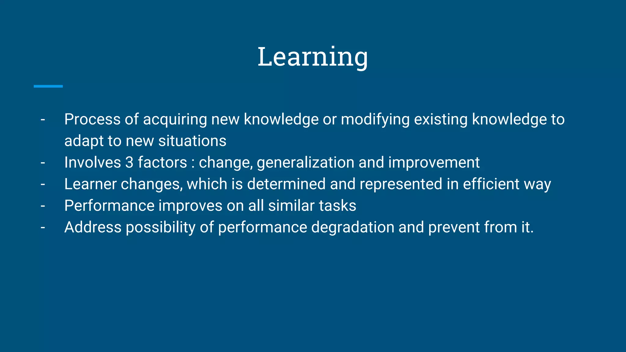
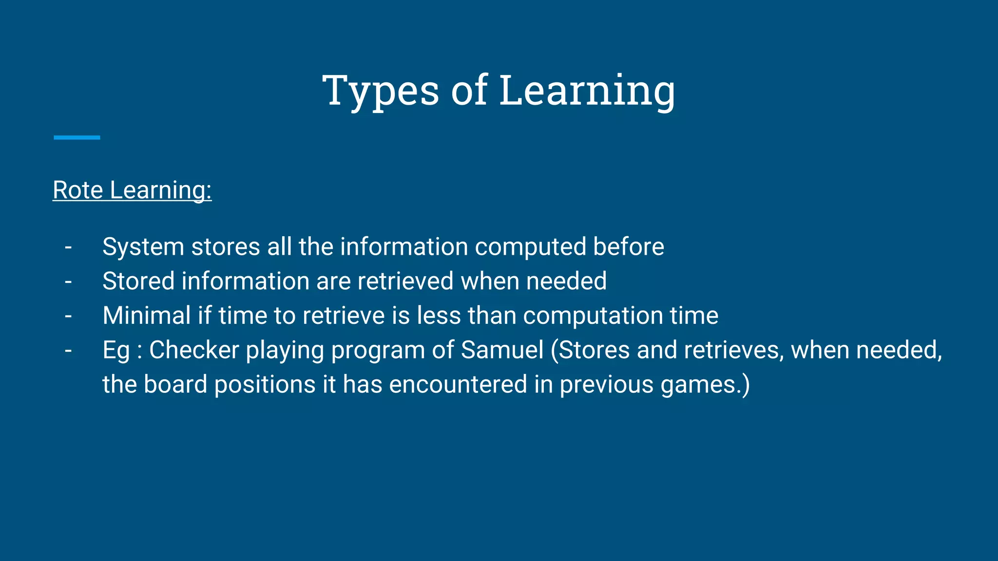
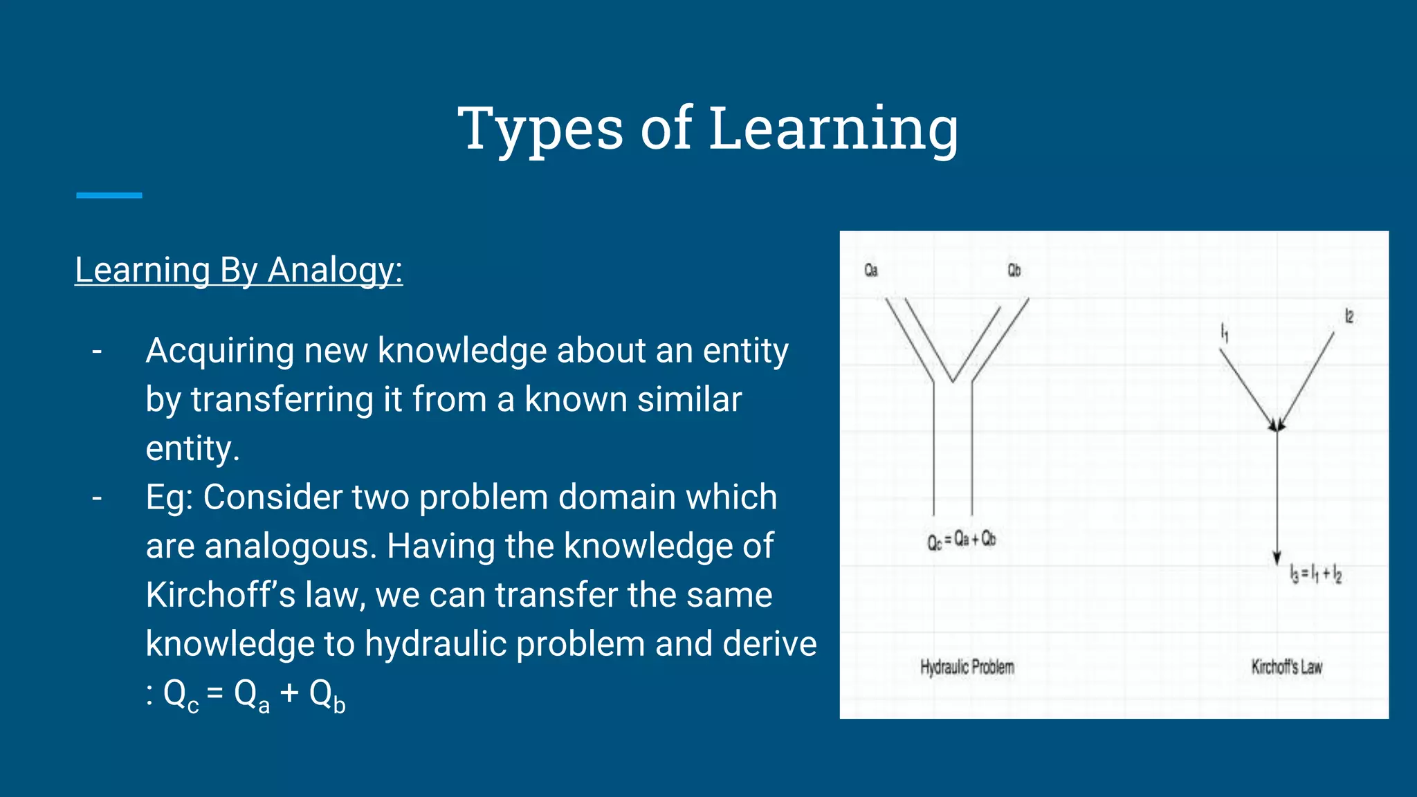
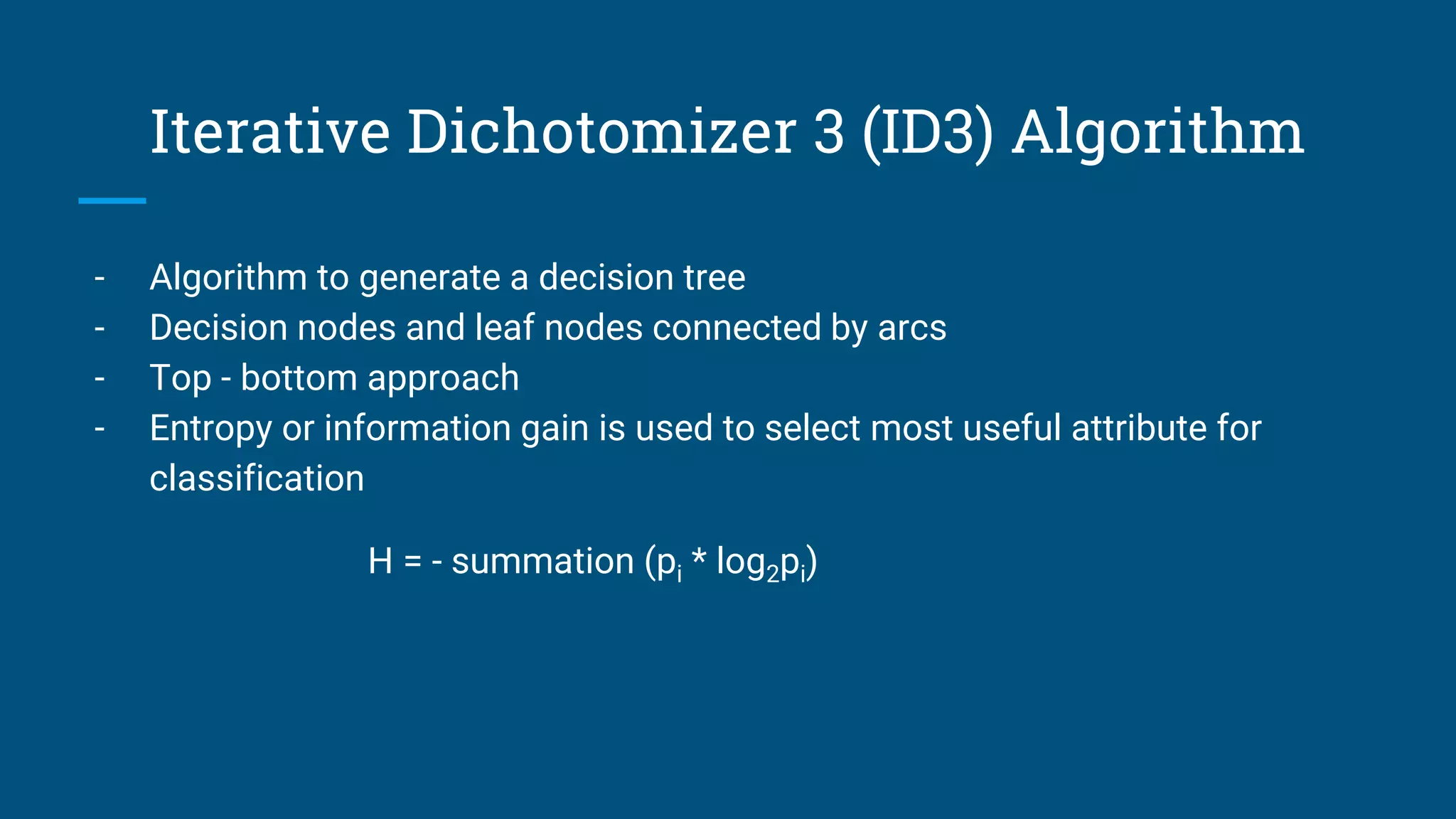
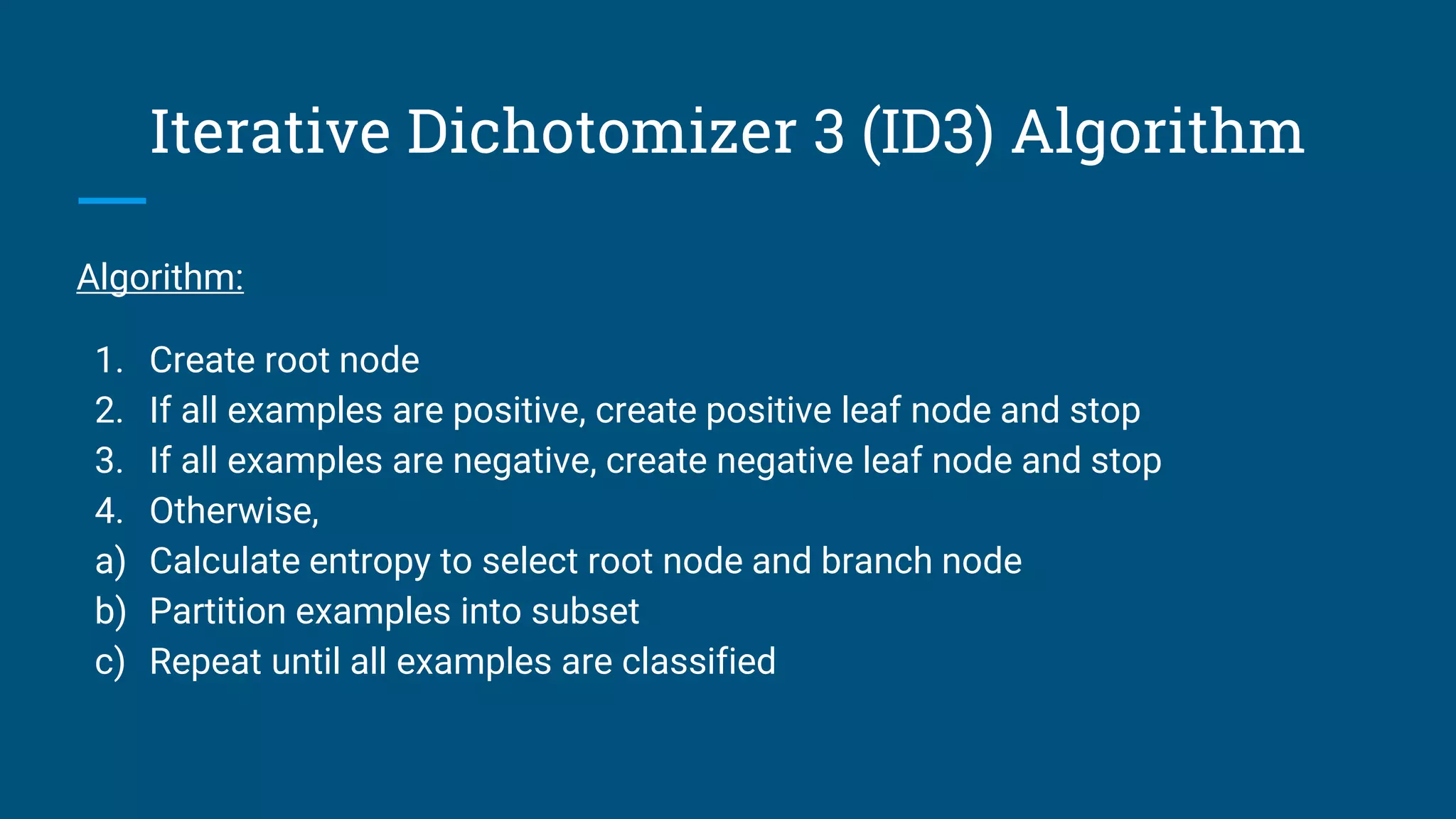
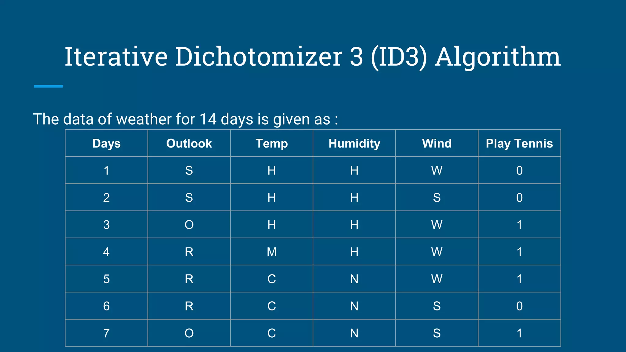
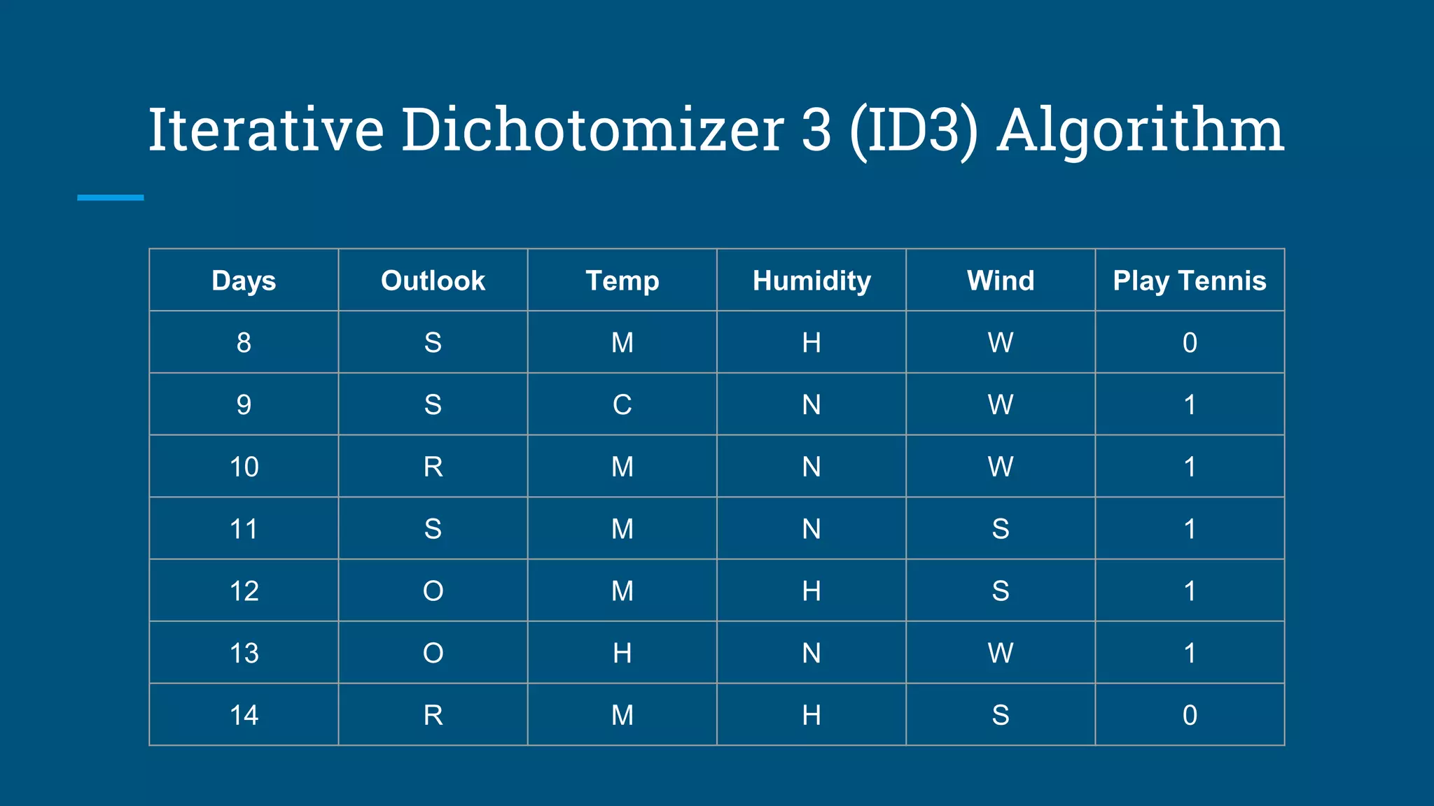
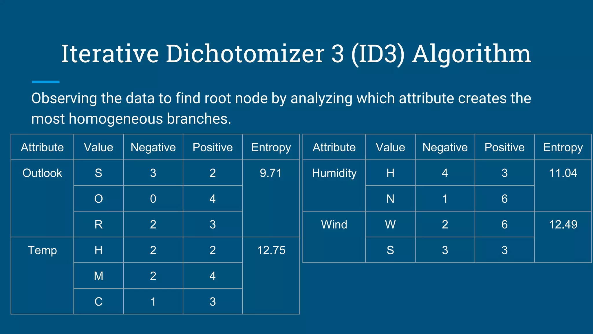
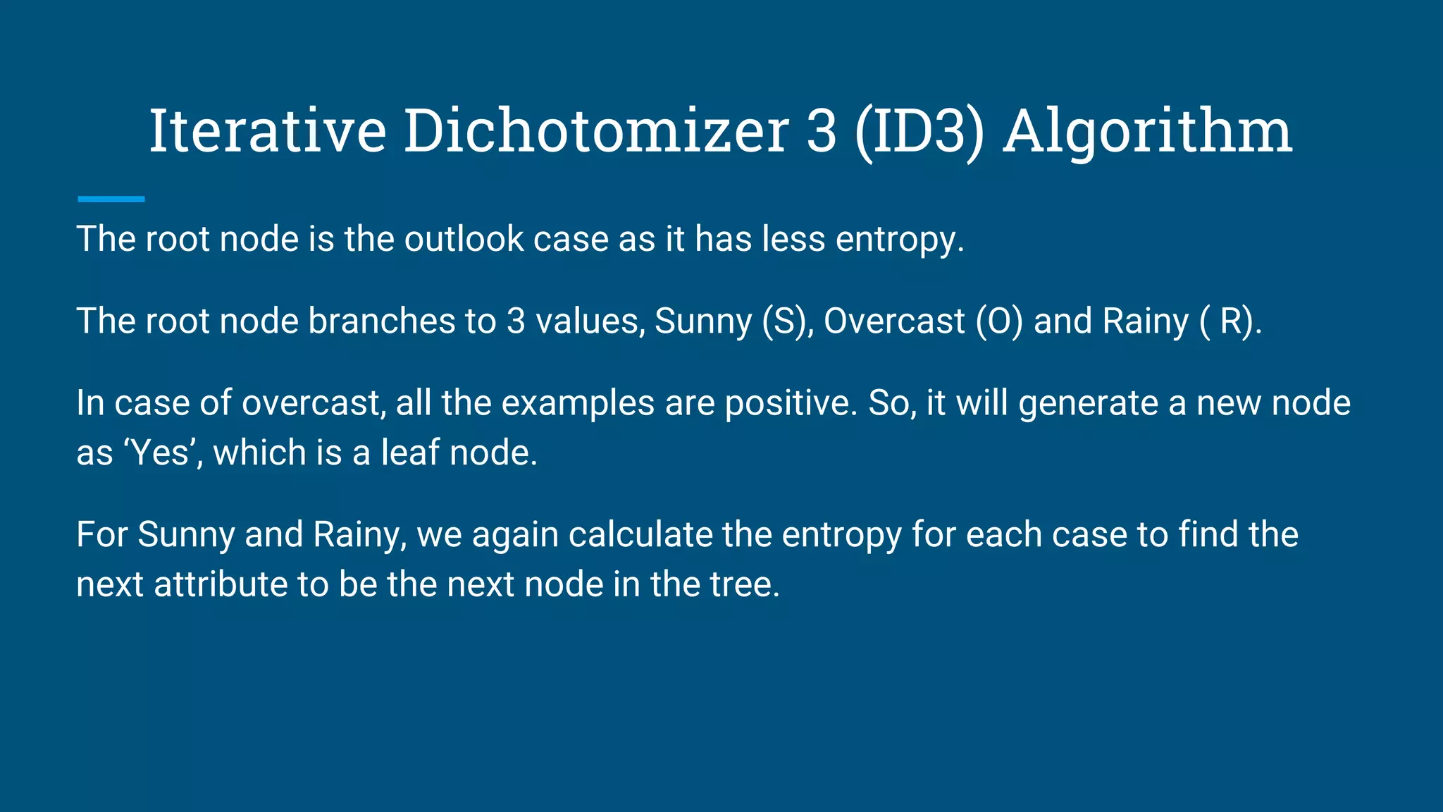
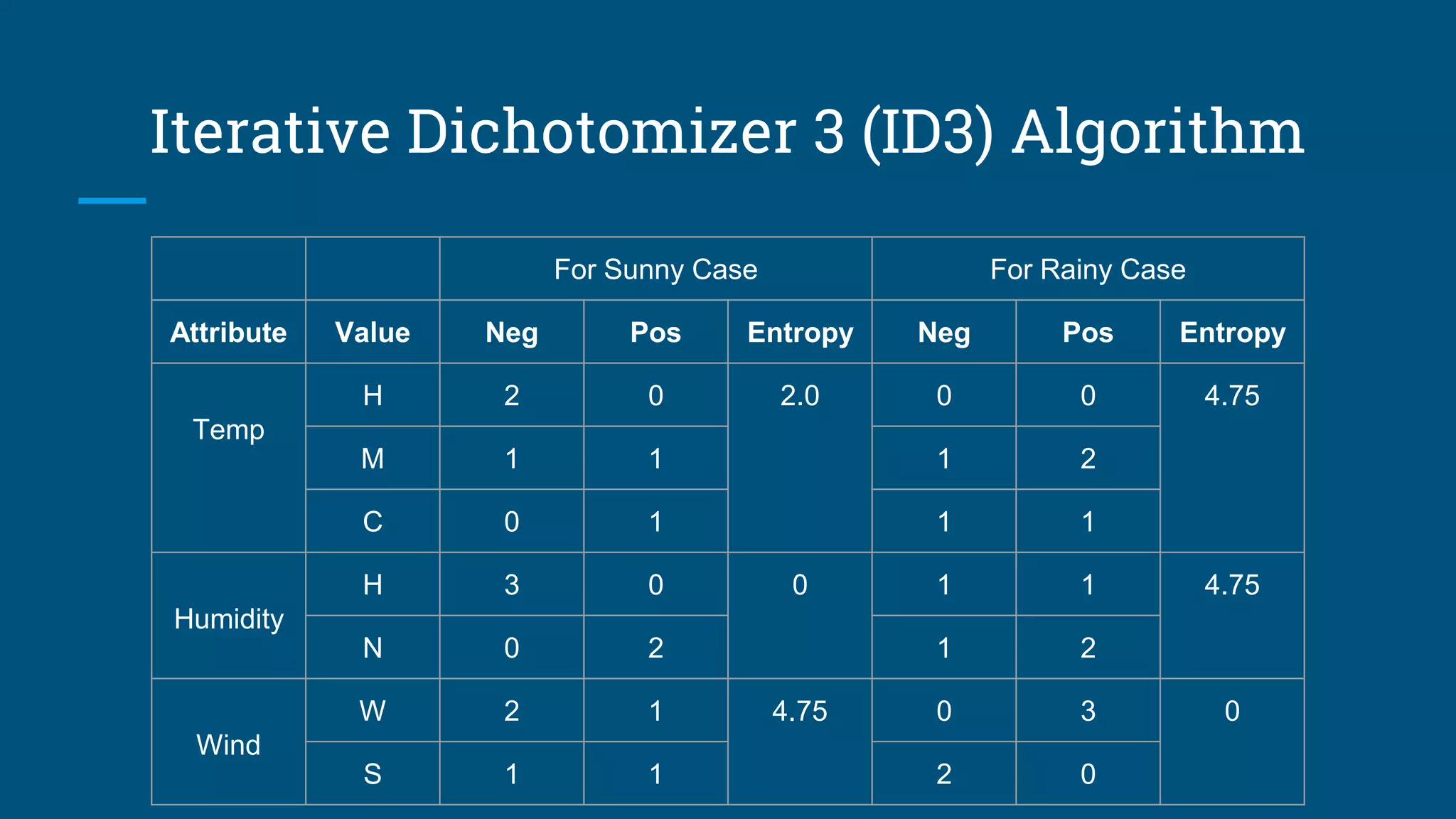
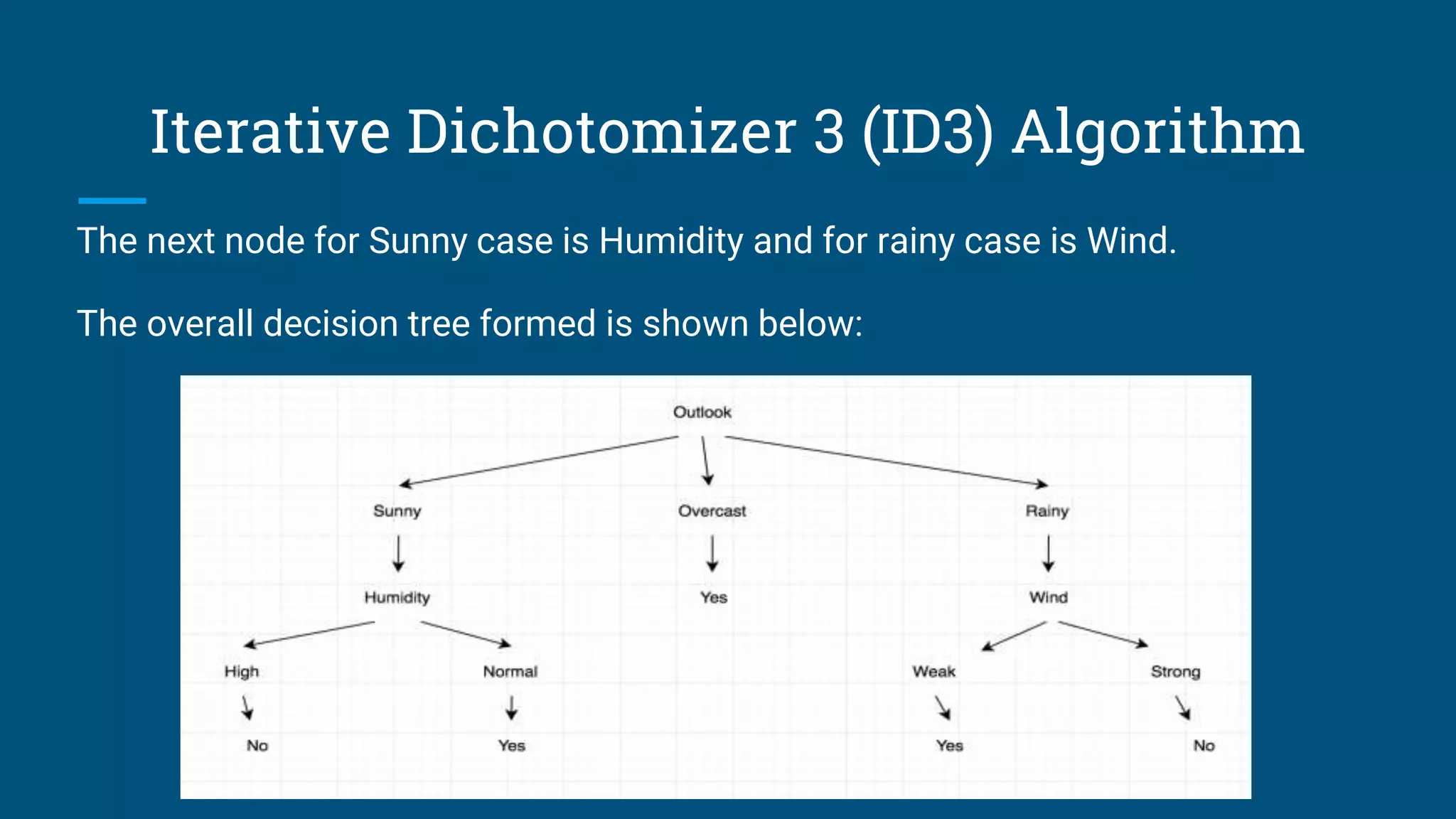
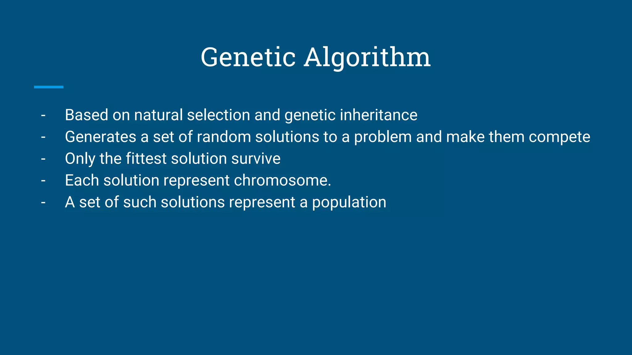
The document discusses various machine learning techniques, including rote learning, learning by analogy, explanation-based learning, and inductive learning using the Iterative Dichotomizer 3 (ID3) algorithm for decision tree generation. It also covers genetic algorithms for optimization, fuzzy inference systems for context-dependent knowledge representation, and Boltzmann machines as stochastic neural networks. Each method is explained with examples and algorithms, showcasing their applications and key principles.