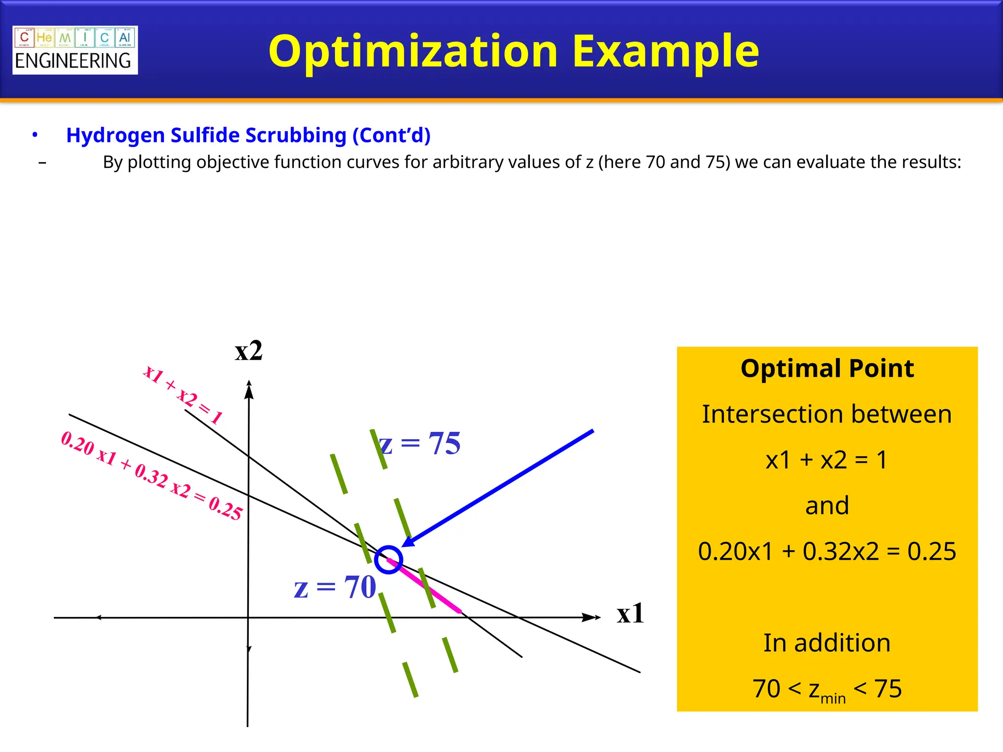
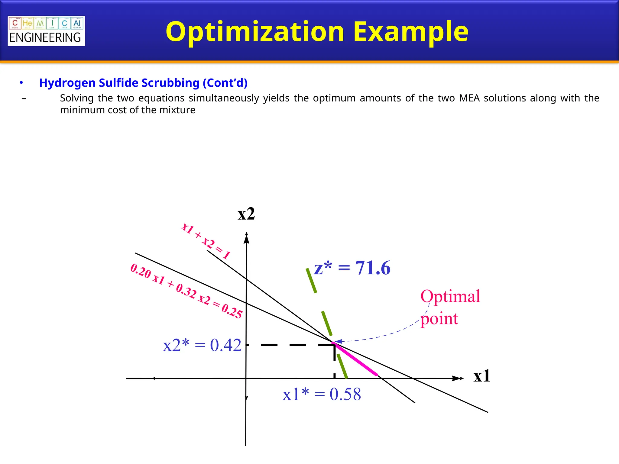
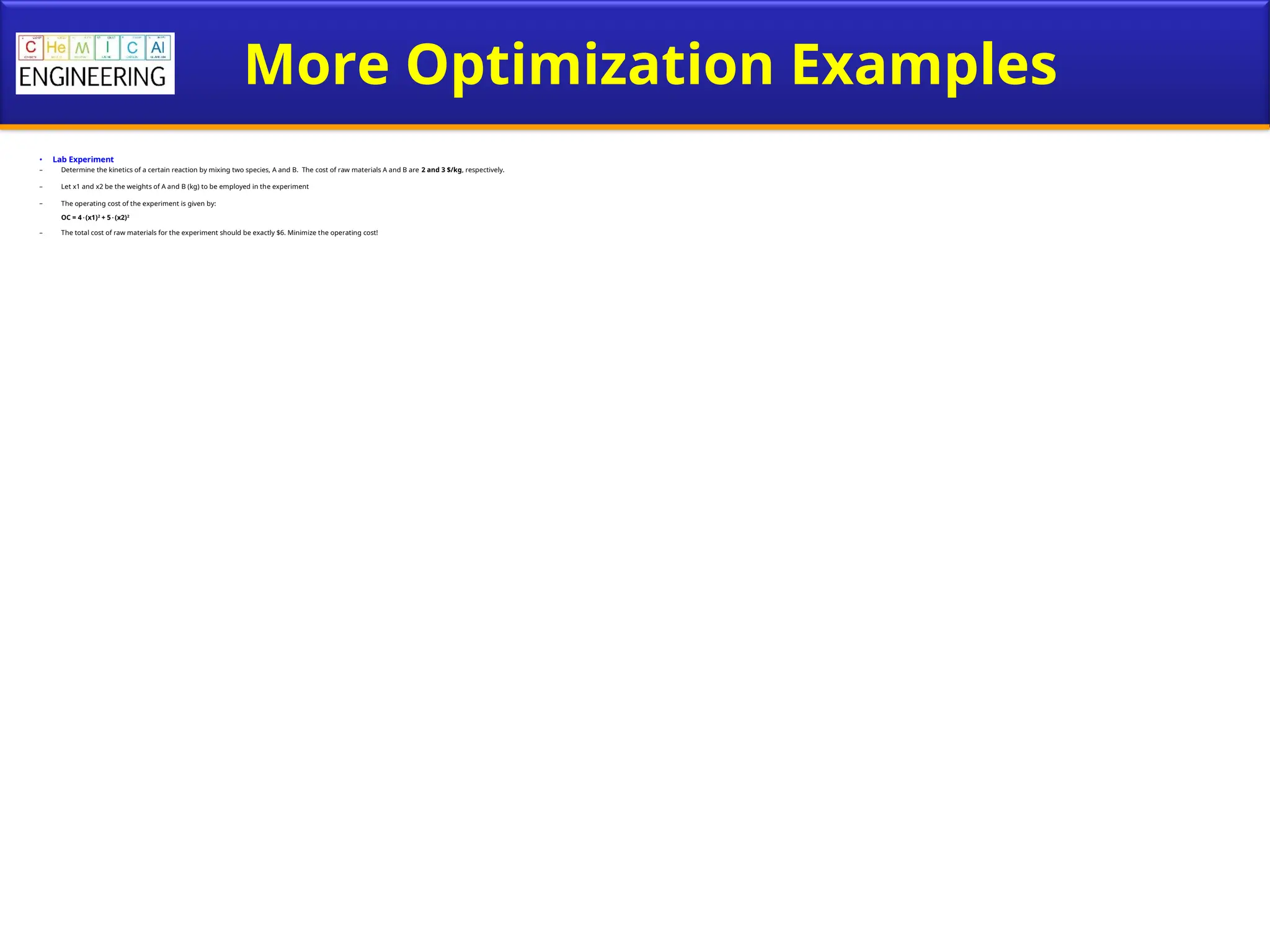
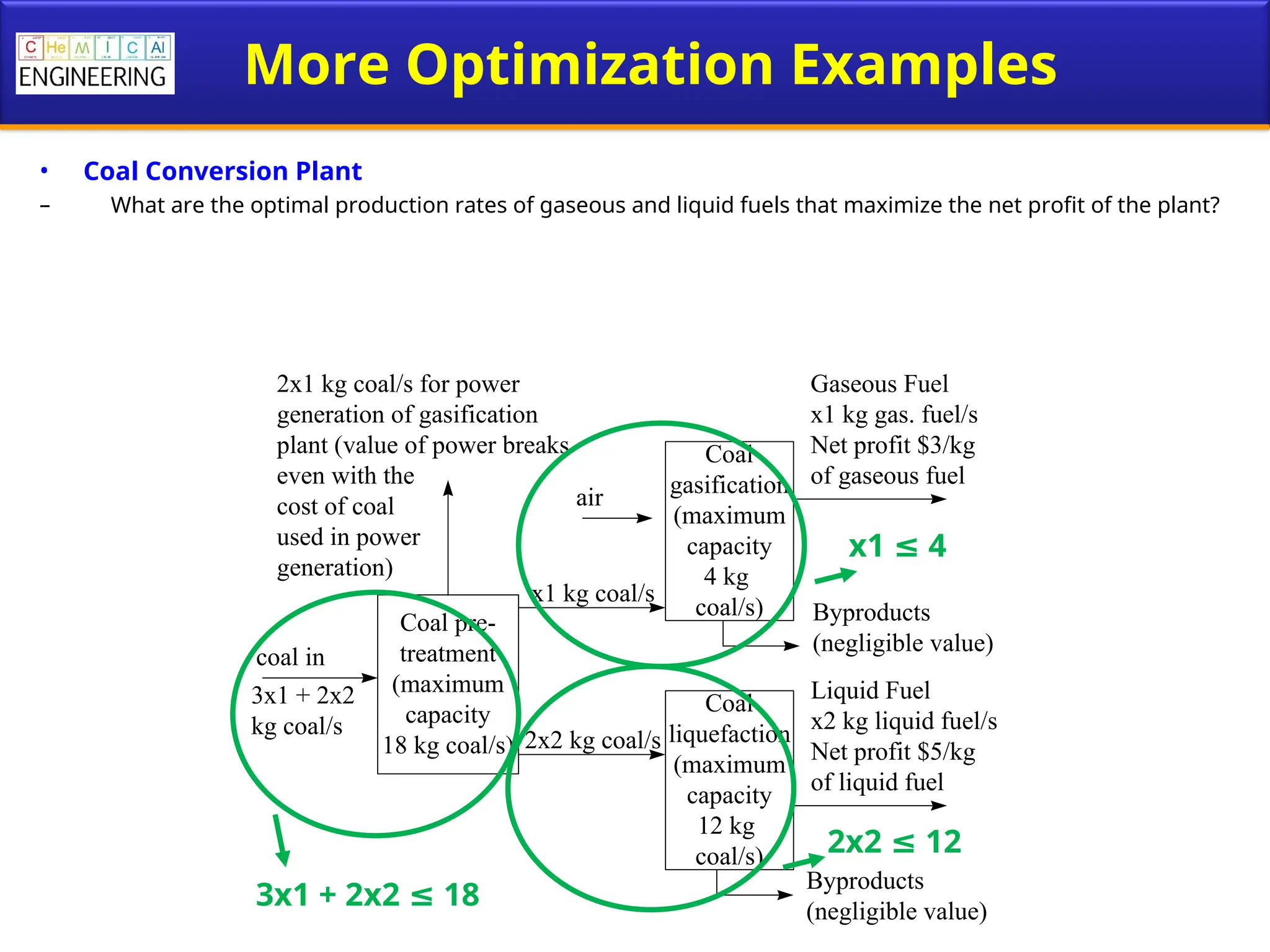
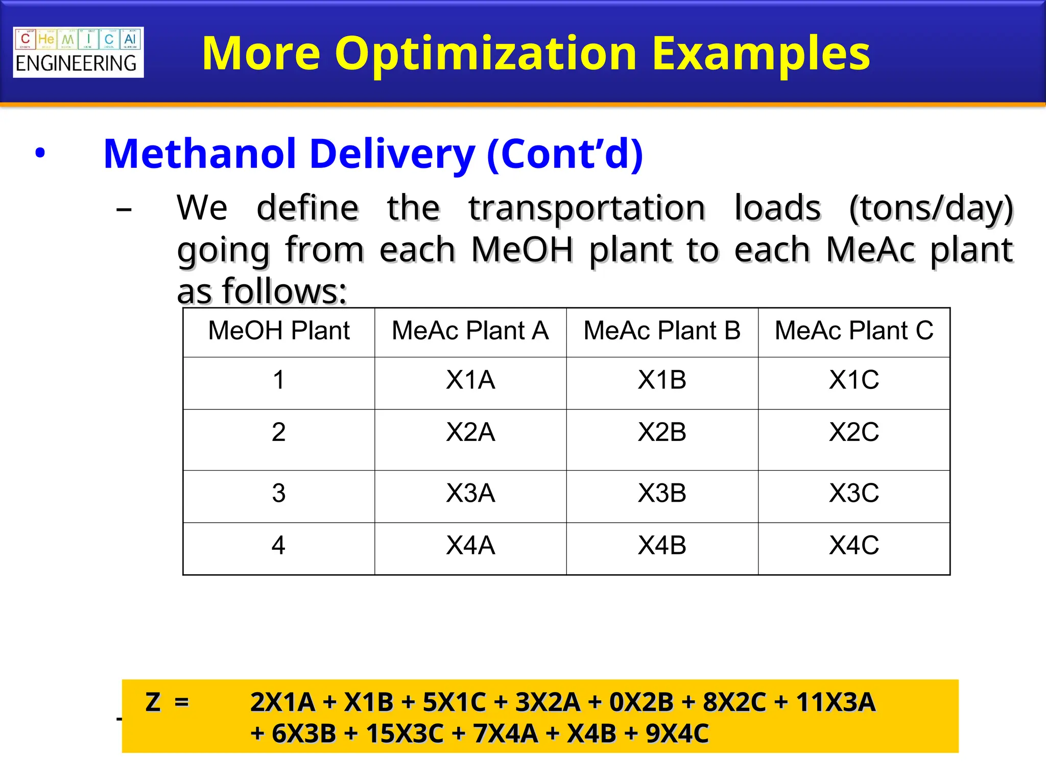
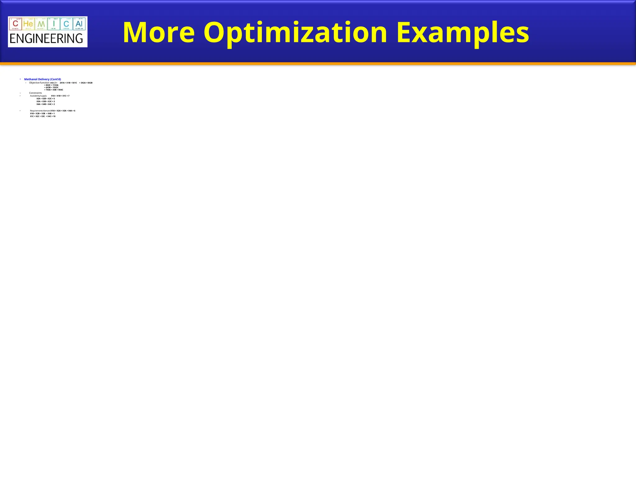
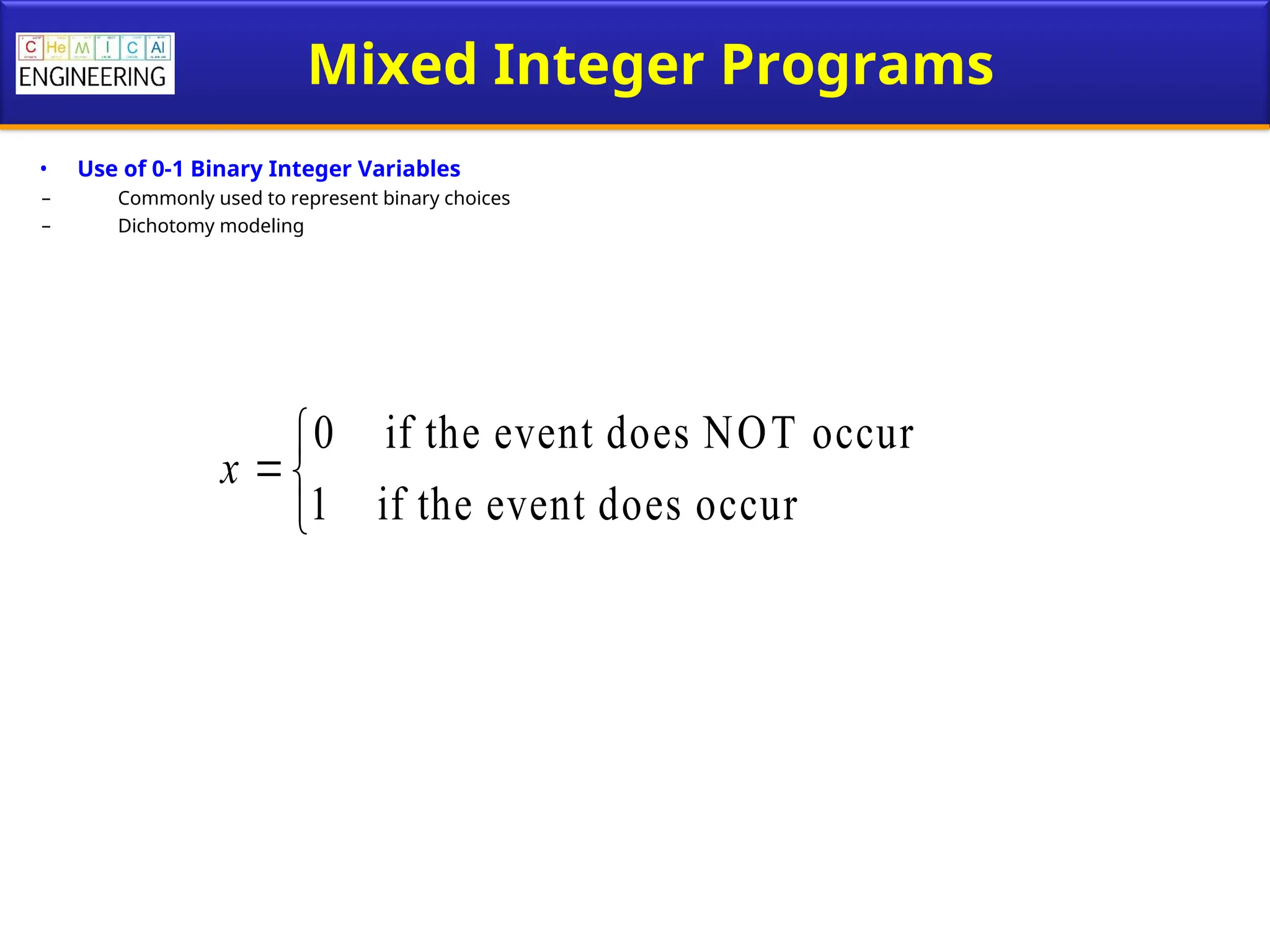
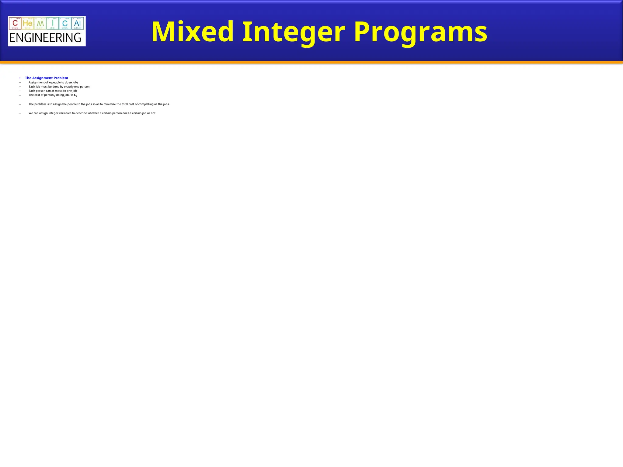
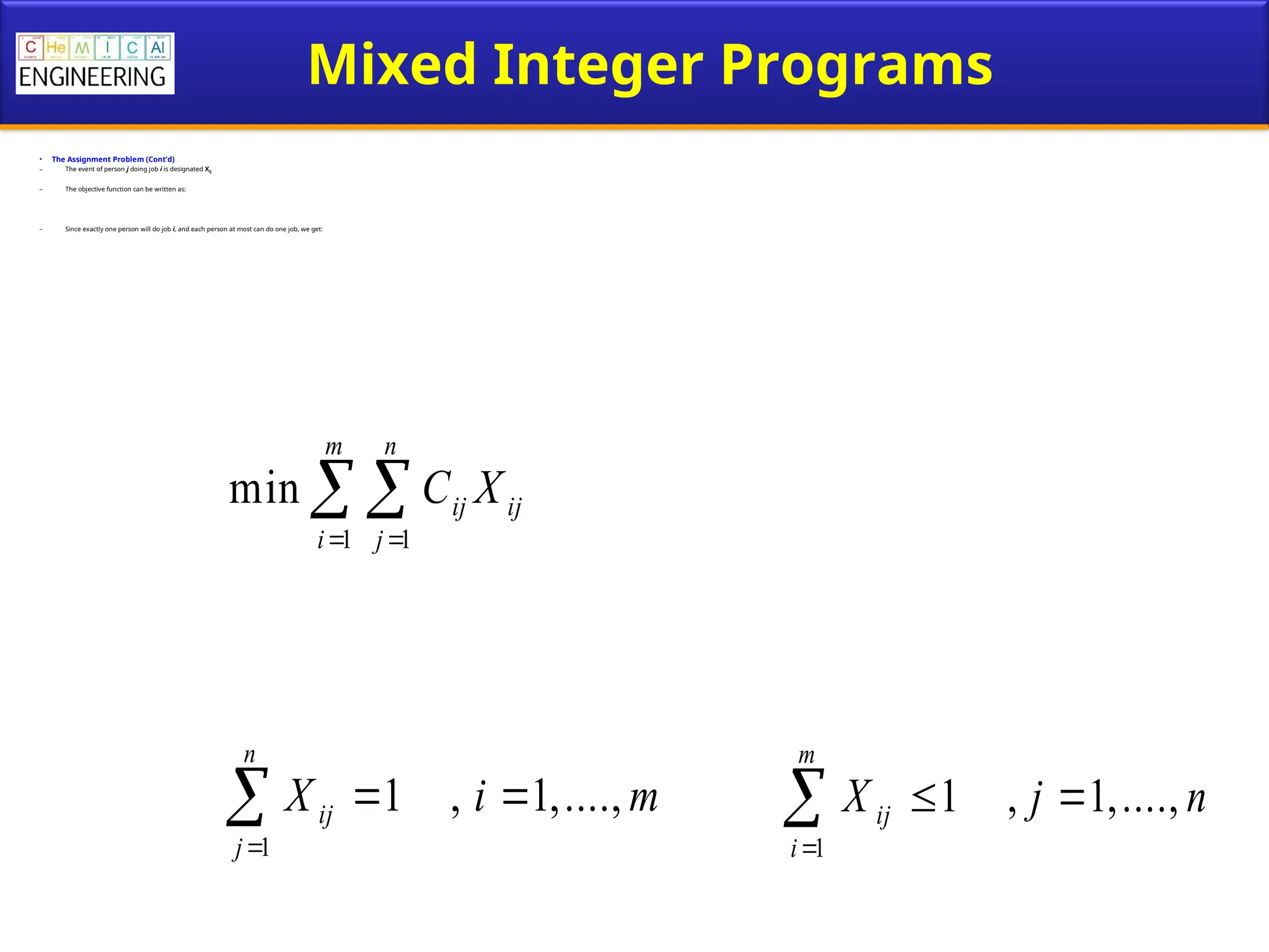
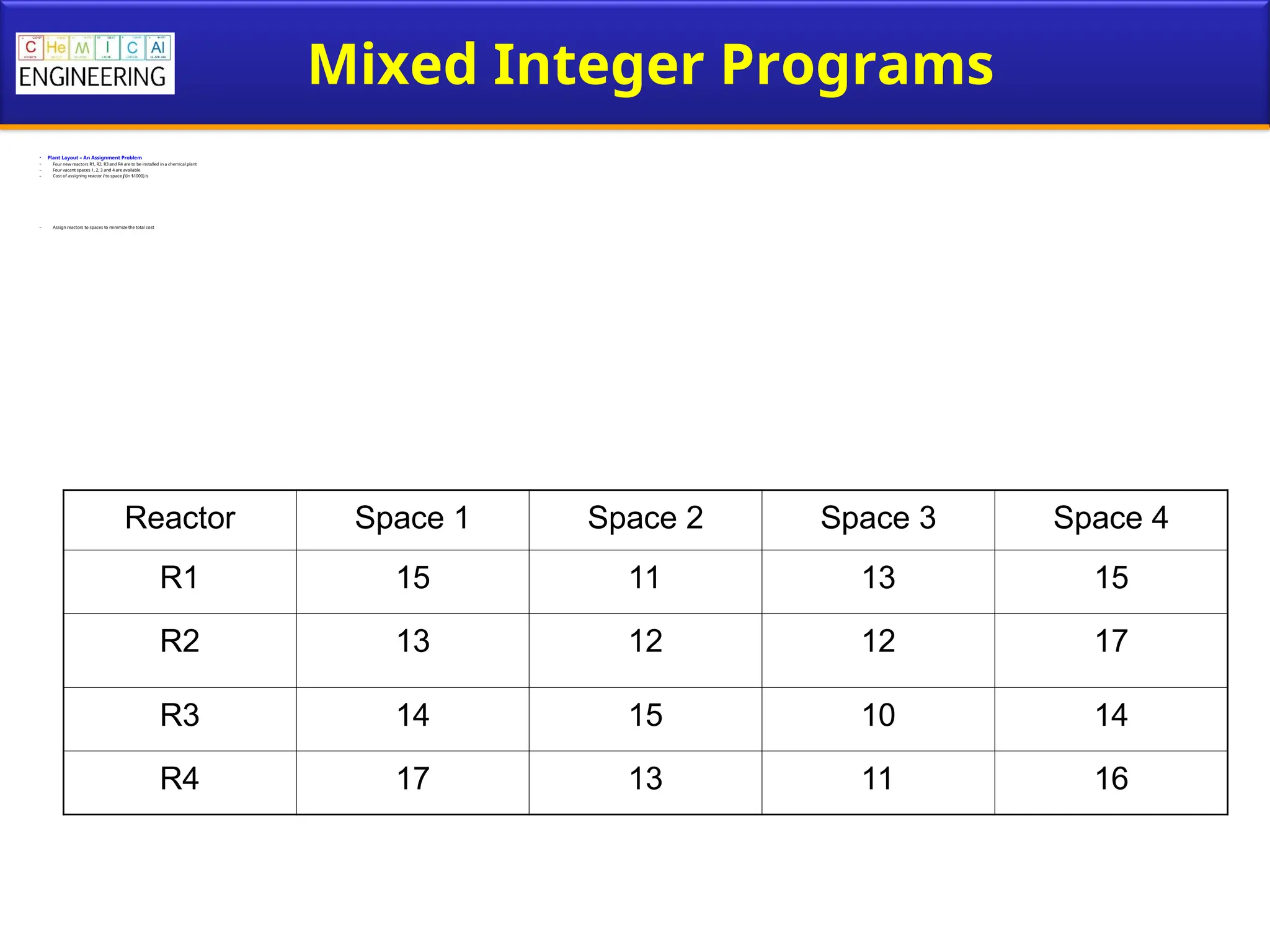
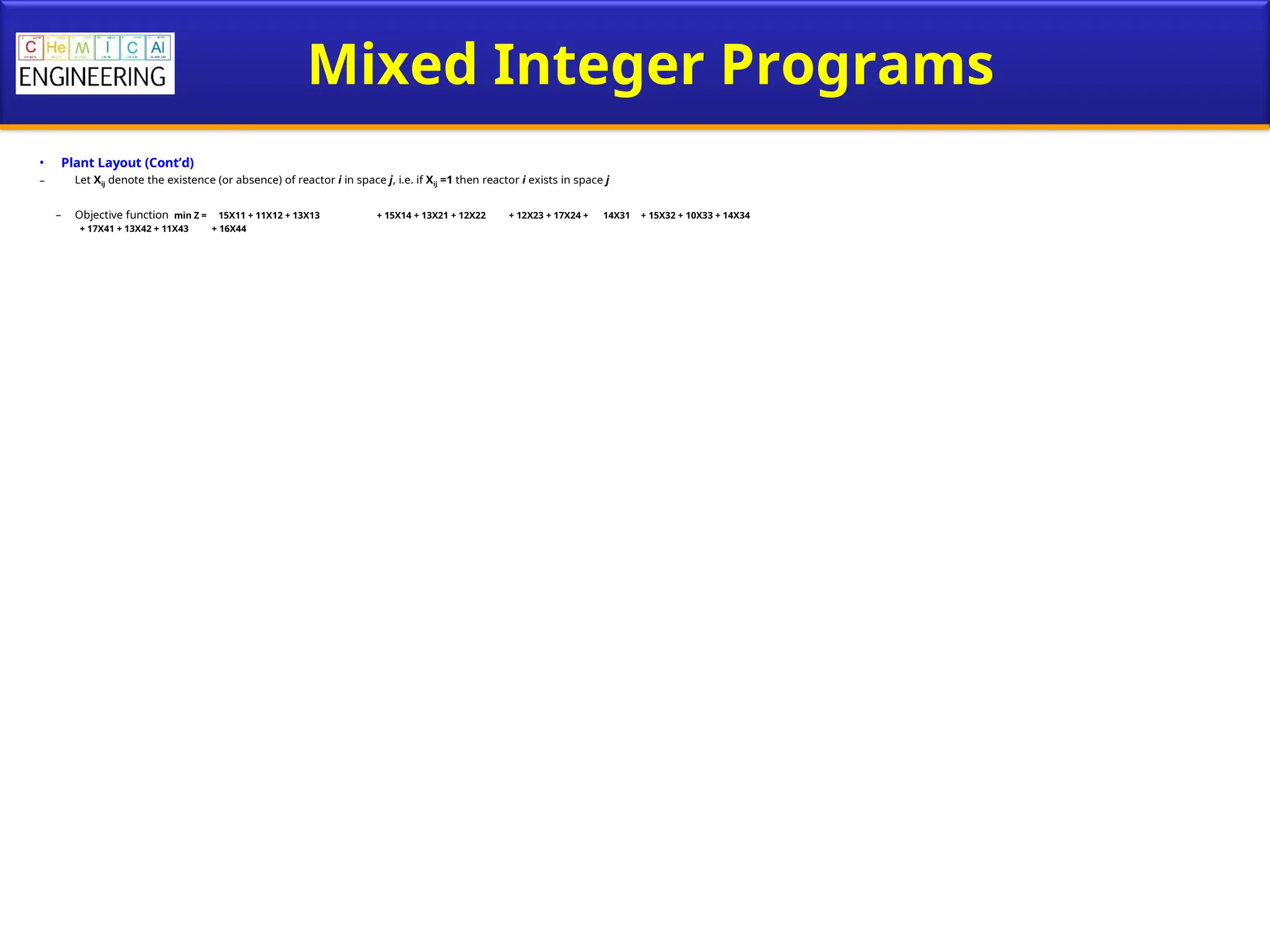
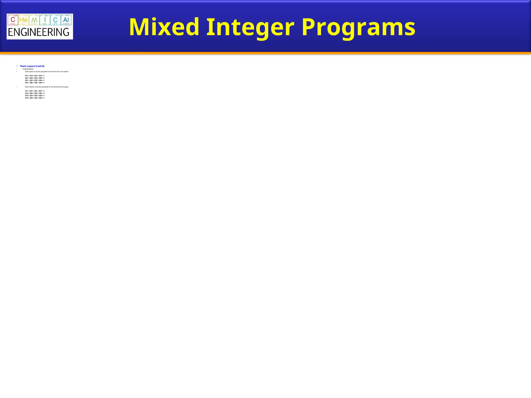
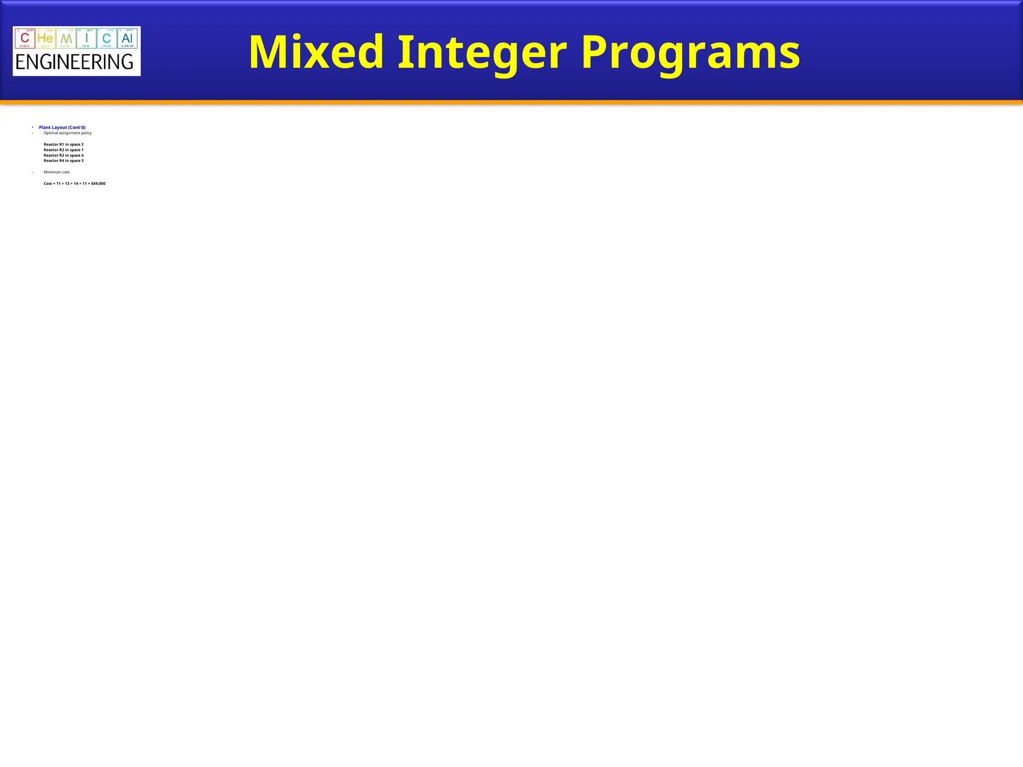
The material used in this presentation i.e., pictures/graphs/text, etc. is solely
intended for educational/teaching purpose, offered free of cost to the students
for use under special circumstances of Online Education due to COVID-19
Lockdown situation and may include copyrighted material - the use of which
may not have been specifically authorized by Copyright Owners. It’s
application constitutes Fair Use of any such copyrighted material as provided
in globally accepted law of many countries. The contents of presentations are
intended only for the attendees of the class being conducted by the presenter.
Fair Use Notice
Optimization
Chemical Process Design and
Simulation
Dr. Imran Nazir Unar
Department of Chemical Engineering
MUET Jamshoro
Lecture No. 6 – Mathematical Optimization
Lecture 6 – Objective
 Understand the different types of optimization
problems and their formulation
On completion of this part, you should:
Optimization Basics
• What is Optimization?
– The purpose of optimization is to maximize (or minimize) the value of a function (called objective function) subject to a number of restrictions (called constraints).
• Examples
1.Maximize reactor conversion
Subject to reactor modeling equations
kinetic equations
limitations on T, P and x
Optimization Basics
• Examples (Continued)
2.Minimize cost of plant
Subject to mass & energy balance equations
equipment modeling equations
environmental, technical and logical constraints
Optimization Basics
• Examples (Continued)
3.Maximize your grade in this course
Subject to extracurricular activities
full-time-job requirements
constant demand by other courses and/or your advisor/boss
Optimization Basics
• Formulation of Optimization Problems
min (or max) f(x1,x2,……,xN)
subject to g1(x1,x2,……,xN) 0
≤
g2(x1,x2,……,xN) 0
≤
gm(x1,x2,……,xN) 0
≤
h1(x1,x2,……,xN)=0
h2(x1,x2,……,xN)=0
hE(x1,x2,……,xN)=0
Inequality
Constraints
Equality
Constraints
Feasibility
Any vector (or point)
which satisfies all the
constraints of the
optimization program is
called a feasible vector
(or a feasible point)
The set of all feasible
points is called feasibility
region or feasibility
domain
Any optimal solution
must lie within the
Optimization Basics
• Classification of Optimization Problems
– Linear Programs (LP’s)
• A mathematical program is linear if
f(x1,x2,……,xN) and gi(x1,x2,……,xN) 0 are
≤ linear in each of their arguments:
f(x1,x2,……,xN) = c1x1 + c2x2 + …. cNxN
gi(x1,x2,……,xN) = ai1x1 + ai2x2 + …. aiNxN
where ci and aij are known constants.
Linear Programs (LP’s) can be solved to yield a
global optimum. Solver routines can guarantee a
truly optimal solution.
Optimization Basics
• Classification of Optimization Problems
– Non-Linear Programs (NLP’s)
• A mathematical program is non-linear if any of the arguments are non-linear. For example:
min 3x + 6y2
s.t. 5x + xy 0
≥
– Integer Programming
• Optimization programs in whichALL the variables must assume integer values. The most commonly used integer variables are the zero/one binary integer variables.
• Integer variables are often used as decision variables, e.g. to choose between two reactor types.
Non-Linear Programs (NLP’s) can
be solved to yield a local
optimum. Solver routines can
not always guarantee a globally
optimal solution.
Optimization Basics
• Classification of Optimization Problems
– Mixed Integer Linear Programs (MILP’s)
• Linear programs in which SOME of the variables are real and other variables are integers
• Can be solved as individual LP’s by fixing the integer variables, thus a global optimum can be identified.
– Mixed Integer Non-Linear Programs (MINLP’s)
• Non-linear programs in which SOME of the variables are real and other variables are integers
• Can be solved as individual NLP’s by fixing the integer variables, but depending on the nature of the NLP’s it may not be possible to find a global optimum.
Optimization Basics
• Formulation of Optimization Problems
– Step 1
• Determine the quantity to be optimized and express it as a mathematical function (this is your objective function)
• Doing so also serves to define variables to be optimized (input variables or optimization variables)
– Step 2
• Identify all stipulated requirements, restrictions, and limitations, and express them mathematically. These requirements constitute the constraints
– Step 3
• Express any hidden conditions. Such conditions are not stipulated explicitly in the problem, but are apparent from the physical situation, e.g. non-negativity constraints
Optimization Example
• Hydrogen Sulfide Scrubbing
– Two variable grades of MEA.
– First grade consists of 80 weight% MEA and 20% weight water. Its cost is 80 cent/kg.
– Second grade consists of 68 weight% MEA and 32 weight% water. Its cost is 60 cent/kg.
– It is desired to mix the two grades so as to obtain an MEA solution that contains no more than 25 weight% water.
– What is the optimal mixing ratio of the two grades which will minimize the cost of MEA solution (per kg)?
Optimization Example
• Hydrogen Sulfide Scrubbing (Cont’d)
– Objective function min z = 80x1 + 60x2
– Constraints
• Water content limitation 0.20x1 + 0.32x2 0.25
≤
• Overall material balance x1 + x2 =1
• Non-negativity x1 ≥ 0
x2 ≥ 0
MIXER
Grade 1
x1 kg
0.80 MEA, 0.20 water
80 cents/kg
Grade 2
x2 kg
0.68 MEA, 0.32 water
60 cents/kg
1 kg MEA solution
water content 25 wt. %

Variables (Basis 1 kg solution)
x1 Amount of grade 1 (kg)
x2 Amount of grade 2 (kg)
z Cost of 1 kg solution (cents)
Optimization Example
• Hydrogen Sulfide Scrubbing (Cont’d)
– Feasibility region
• The set of points (x1, x2) satisfying all the constraints, including the non-negativity conditions.
• Constraint on water content 0.20x1 + 0.32x2 0.25
≤
x2
x1
Optimization Example
• Hydrogen Sulfide Scrubbing (Cont’d)
– Feasibility region
• Non-negativity constraints x1  0 , x2  0
x2
x1
x2
x1
Optimization Example
• Hydrogen Sulfide Scrubbing (Cont’d)
– Feasibility region
• Mass balance constraint x1 + x2 = 1
x2
x1
x2
x1
x2
x1
0.20 x1 + 0.32 x2 = 0.25
x1 + x2 = 1
Optimization Example
• Hydrogen Sulfide Scrubbing (Cont’d)
– Feasibility region
x2
x1
0.20 x1 + 0.32 x2 = 0.25
x1 + x2 = 1
Feasibility region
is this heavy line
Any optimal solution
must lie within the
feasibility region!
Optimization Example
• Hydrogen Sulfide Scrubbing (Cont’d)
– By plotting objective function curves for arbitrary values of z (here 70 and 75) we can evaluate the results:
x2
x1
0.20 x1 + 0.32 x2 = 0.25
x1 + x2 = 1
z = 75
z = 70
Optimal Point
Intersection between
x1 + x2 = 1
and
0.20x1 + 0.32x2 = 0.25
In addition
70 < zmin < 75
Optimization Example
• Hydrogen Sulfide Scrubbing (Cont’d)
– Solving the two equations simultaneously yields the optimum amounts of the two MEA solutions along with the
minimum cost of the mixture
x2
x1
0.20 x1 + 0.32 x2 = 0.25
x1 + x2 = 1
z* = 71.6
Optimal
point
x2* = 0.42
x1* = 0.58
More Optimization Examples
• Lab Experiment
– Determine the kinetics of a certain reaction by mixing two species, A and B. The cost of raw materials A and B are 2 and 3 $/kg, respectively.
– Let x1 and x2 be the weights of A and B (kg) to be employed in the experiment
– The operating cost of the experiment is given by:
OC = 4(x1)2
+ 5(x2)2
– The total cost of raw materials for the experiment should be exactly $6. Minimize the operating cost!
More Optimization Examples
• Coal Conversion Plant
– What are the optimal production rates of gaseous and liquid fuels that maximize the net profit of the plant?
Coal pre-
treatment
(maximum
capacity
18 kg coal/s)
Coal
gasification
(maximum
capacity
4 kg
coal/s)
coal in
3x1 + 2x2
kg coal/s
2x1 kg coal/s for power
generation of gasification
plant (value of power breaks
even with the
cost of coal
used in power
generation)
air
x1 kg coal/s
Coal
liquefaction
(maximum
capacity
12 kg
coal/s)
Byproducts
(negligible value)
Gaseous Fuel
x1 kg gas. fuel/s
Net profit $3/kg
of gaseous fuel
2x2 kg coal/s
Byproducts
(negligible value)
Liquid Fuel
x2 kg liquid fuel/s
Net profit $5/kg
of liquid fuel
3x1 + 2x2 18
≤
x1 4
≤
2x2 12
≤
More Optimization Examples
• Coal Conversion Plant (Cont’d)
– Objective function max z = 3x1 + 5x2
– Constraints
• Pretreatment capacity 3x1 + 2x2 18
≤
• Gasification capacity x1 ≤ 4
• Liquefaction capacity 2x2 ≤ 12
• Non-negativity x1 ≥ 0
x2 ≥ 0
0
2
4
6
8
10
0 2 4 6 8
x1
x2
x1 = 4
2x2 = 12
3x1 + 2x2 = 18
More Optimization Examples
• Coal Conversion Plant (Cont’d)
– Graphical solution
Maximum profit Z = 36 for x1 = 2 and x2 = 6
0
2
4
6
8
10
0 2 4 6 8
x1
x2
x1 = 4
2x2 = 12
3x1 + 2x2 = 18
0
2
4
6
8
10
0 2 4 6 8
x1
x2
Z = 36 = 3x1 + 5x2
Z = 20 = 3x1 + 5x2
Z = 10 = 3x1 + 5x2
More Optimization Examples
• Methanol Delivery
– Supply methanol for three Methyl acetate plants located in towns A, B, and C
– Daily methanol requirements for each plant:
MeAc Plant location Tons/day
A 6
B 1
C 10
– Methanol production plants
MeOH plant 1 2 3 4
Capacity 7 5 3 2
More Optimization Examples
• Methanol Delivery (Cont’d)
– Shipping cost (100 $/ton)
– Schedule the methanol delivery system to minimize the transportation cost
MeOH Plant MeAc Plant A MeAc Plant B MeAc Plant C
1 2 1 5
2 3 0 8
3 11 6 15
4 7 1 9
More Optimization Examples
• Methanol Delivery (Cont’d)
– We define the transportation loads (tons/day)
define the transportation loads (tons/day)
going from each MeOH plant to each MeAc plant
as follows:
as follows:
– Total transportation cost (Z)
MeOH Plant MeAc Plant A MeAc Plant B MeAc Plant C
1 X1A X1B X1C
2 X2A X2B X2C
3 X3A X3B X3C
4 X4A X4B X4C
Z =
Z = 2X1A + X1B + 5X1C + 3X2A + 0X2B + 8X2C + 11X3A
2X1A + X1B + 5X1C + 3X2A + 0X2B + 8X2C + 11X3A
+ 6X3B + 15X3C + 7X4A + X4B + 9X4C
More Optimization Examples
• Methanol Delivery (Cont’d)
– Objective function min Z = 2X1A + X1B + 5X1C + 3X2A + 0X2B
+ 8X2C + 11X3A
+ 6X3B + 15X3C
+ 7X4A + X4B + 9X4C
– Constraints
• Availability/supply X1A + X1B + X1C = 7
X2A + X2B + X2C = 5
X3A + X3B + X3C = 3
X4A + X4B + X4C = 2
• Requirements/demand X1A + X2A + X3A + X4A = 6
X1B + X2B + X3B + X4B = 1
X1C + X2C + X3C + X4C = 10
More Optimization Examples
• Methanol Delivery (Cont’d)
– Constraints
• Non-negativity X1A ≥ 0
X1B ≥ 0
X1C ≥ 0
X2A ≥ 0
X2B ≥ 0
X2C ≥ 0
X3A ≥ 0
X3B ≥ 0
X3C ≥ 0
X4A ≥ 0
X4B ≥ 0
X4C ≥ 0
Mixed Integer Programs
• Use of 0-1 Binary Integer Variables
– Commonly used to represent binary choices
– Dichotomy modeling
0 if the event does NOT occur
1 if the event does occur
x



Mixed Integer Programs
• The Assignment Problem
– Assignment of n people to do m jobs
– Each job must be done by exactly one person
– Each person can at most do one job
– The cost of person j doing job i is Cij
– The problem is to assign the people to the jobs so as to minimize the total cost of completing all the jobs.
– We can assign integer variables to describe whether a certain person does a certain job or not
Mixed Integer Programs
• The Assignment Problem (Cont’d)
– The event of person j doing job i is designated Xij
– The objective function can be written as:
– Since exactly one person will do job i, and each person at most can do one job, we get:
1 1
min
m n
ij ij
i j
C X
 
 
1
1 , 1,....,
n
ij
j
X i m

 
 1
1 , 1,....,
m
ij
i
X j n

 

Mixed Integer Programs
• Plant Layout – An Assignment Problem
– Four new reactors R1, R2, R3 and R4 are to be installed in a chemical plant
– Four vacant spaces 1, 2, 3 and 4 are available
– Cost of assigning reactor i to space j (in $1000) is
– Assign reactors to spaces to minimize the total cost
Reactor Space 1 Space 2 Space 3 Space 4
R1 15 11 13 15
R2 13 12 12 17
R3 14 15 10 14
R4 17 13 11 16
Mixed Integer Programs
• Plant Layout (Cont’d)
– Let Xij denote the existence (or absence) of reactor i in space j, i.e. if Xij =1 then reactor i exists in space j
– Objective function min Z = 15X11 + 11X12 + 13X13 + 15X14 + 13X21 + 12X22 + 12X23 + 17X24 + 14X31 + 15X32 + 10X33 + 14X34
+ 17X41 + 13X42 + 11X43 + 16X44
Mixed Integer Programs
• Plant Layout (Cont’d)
– Constraints
• Each space must be assigned to one and only one reactor
X11 + X12 + X13 + X14 = 1
X21 + X22 + X23 + X24 = 1
X31 + X32 + X33 + X34 = 1
X41 + X42 + X43 + X44 = 1
• Each reactor must be assigned to one and only one space
X11 + X21 + X31 + X41 = 1
X12 + X22 + X32 + X42 = 1
X13 + X23 + X33 + X43 = 1
X14 + X24 + X34 + X44 = 1
Mixed Integer Programs
• Plant Layout (Cont’d)
– Optimal assignment policy
Reactor R1 in space 2
Reactor R2 in space 1
Reactor R3 in space 4
Reactor R4 in space 3
– Minimum cost
Cost = 11 + 13 + 14 + 11 = $49,000
Mixed Integer Programs
Thank You

Lecture-4-Mathematical Optimization_This.ppt

  • 1.
    The material usedin this presentation i.e., pictures/graphs/text, etc. is solely intended for educational/teaching purpose, offered free of cost to the students for use under special circumstances of Online Education due to COVID-19 Lockdown situation and may include copyrighted material - the use of which may not have been specifically authorized by Copyright Owners. It’s application constitutes Fair Use of any such copyrighted material as provided in globally accepted law of many countries. The contents of presentations are intended only for the attendees of the class being conducted by the presenter. Fair Use Notice
  • 2.
    Optimization Chemical Process Designand Simulation Dr. Imran Nazir Unar Department of Chemical Engineering MUET Jamshoro Lecture No. 6 – Mathematical Optimization
  • 3.
    Lecture 6 –Objective  Understand the different types of optimization problems and their formulation On completion of this part, you should:
  • 4.
    Optimization Basics • Whatis Optimization? – The purpose of optimization is to maximize (or minimize) the value of a function (called objective function) subject to a number of restrictions (called constraints). • Examples 1.Maximize reactor conversion Subject to reactor modeling equations kinetic equations limitations on T, P and x
  • 5.
    Optimization Basics • Examples(Continued) 2.Minimize cost of plant Subject to mass & energy balance equations equipment modeling equations environmental, technical and logical constraints
  • 6.
    Optimization Basics • Examples(Continued) 3.Maximize your grade in this course Subject to extracurricular activities full-time-job requirements constant demand by other courses and/or your advisor/boss
  • 7.
    Optimization Basics • Formulationof Optimization Problems min (or max) f(x1,x2,……,xN) subject to g1(x1,x2,……,xN) 0 ≤ g2(x1,x2,……,xN) 0 ≤ gm(x1,x2,……,xN) 0 ≤ h1(x1,x2,……,xN)=0 h2(x1,x2,……,xN)=0 hE(x1,x2,……,xN)=0 Inequality Constraints Equality Constraints Feasibility Any vector (or point) which satisfies all the constraints of the optimization program is called a feasible vector (or a feasible point) The set of all feasible points is called feasibility region or feasibility domain Any optimal solution must lie within the
  • 8.
    Optimization Basics • Classificationof Optimization Problems – Linear Programs (LP’s) • A mathematical program is linear if f(x1,x2,……,xN) and gi(x1,x2,……,xN) 0 are ≤ linear in each of their arguments: f(x1,x2,……,xN) = c1x1 + c2x2 + …. cNxN gi(x1,x2,……,xN) = ai1x1 + ai2x2 + …. aiNxN where ci and aij are known constants. Linear Programs (LP’s) can be solved to yield a global optimum. Solver routines can guarantee a truly optimal solution.
  • 9.
    Optimization Basics • Classificationof Optimization Problems – Non-Linear Programs (NLP’s) • A mathematical program is non-linear if any of the arguments are non-linear. For example: min 3x + 6y2 s.t. 5x + xy 0 ≥ – Integer Programming • Optimization programs in whichALL the variables must assume integer values. The most commonly used integer variables are the zero/one binary integer variables. • Integer variables are often used as decision variables, e.g. to choose between two reactor types. Non-Linear Programs (NLP’s) can be solved to yield a local optimum. Solver routines can not always guarantee a globally optimal solution.
  • 10.
    Optimization Basics • Classificationof Optimization Problems – Mixed Integer Linear Programs (MILP’s) • Linear programs in which SOME of the variables are real and other variables are integers • Can be solved as individual LP’s by fixing the integer variables, thus a global optimum can be identified. – Mixed Integer Non-Linear Programs (MINLP’s) • Non-linear programs in which SOME of the variables are real and other variables are integers • Can be solved as individual NLP’s by fixing the integer variables, but depending on the nature of the NLP’s it may not be possible to find a global optimum.
  • 11.
    Optimization Basics • Formulationof Optimization Problems – Step 1 • Determine the quantity to be optimized and express it as a mathematical function (this is your objective function) • Doing so also serves to define variables to be optimized (input variables or optimization variables) – Step 2 • Identify all stipulated requirements, restrictions, and limitations, and express them mathematically. These requirements constitute the constraints – Step 3 • Express any hidden conditions. Such conditions are not stipulated explicitly in the problem, but are apparent from the physical situation, e.g. non-negativity constraints
  • 12.
    Optimization Example • HydrogenSulfide Scrubbing – Two variable grades of MEA. – First grade consists of 80 weight% MEA and 20% weight water. Its cost is 80 cent/kg. – Second grade consists of 68 weight% MEA and 32 weight% water. Its cost is 60 cent/kg. – It is desired to mix the two grades so as to obtain an MEA solution that contains no more than 25 weight% water. – What is the optimal mixing ratio of the two grades which will minimize the cost of MEA solution (per kg)?
  • 13.
    Optimization Example • HydrogenSulfide Scrubbing (Cont’d) – Objective function min z = 80x1 + 60x2 – Constraints • Water content limitation 0.20x1 + 0.32x2 0.25 ≤ • Overall material balance x1 + x2 =1 • Non-negativity x1 ≥ 0 x2 ≥ 0 MIXER Grade 1 x1 kg 0.80 MEA, 0.20 water 80 cents/kg Grade 2 x2 kg 0.68 MEA, 0.32 water 60 cents/kg 1 kg MEA solution water content 25 wt. %  Variables (Basis 1 kg solution) x1 Amount of grade 1 (kg) x2 Amount of grade 2 (kg) z Cost of 1 kg solution (cents)
  • 14.
    Optimization Example • HydrogenSulfide Scrubbing (Cont’d) – Feasibility region • The set of points (x1, x2) satisfying all the constraints, including the non-negativity conditions. • Constraint on water content 0.20x1 + 0.32x2 0.25 ≤ x2 x1
  • 15.
    Optimization Example • HydrogenSulfide Scrubbing (Cont’d) – Feasibility region • Non-negativity constraints x1  0 , x2  0 x2 x1 x2 x1
  • 16.
    Optimization Example • HydrogenSulfide Scrubbing (Cont’d) – Feasibility region • Mass balance constraint x1 + x2 = 1 x2 x1 x2 x1 x2 x1 0.20 x1 + 0.32 x2 = 0.25 x1 + x2 = 1
  • 17.
    Optimization Example • HydrogenSulfide Scrubbing (Cont’d) – Feasibility region x2 x1 0.20 x1 + 0.32 x2 = 0.25 x1 + x2 = 1 Feasibility region is this heavy line Any optimal solution must lie within the feasibility region!
  • 18.
    Optimization Example • HydrogenSulfide Scrubbing (Cont’d) – By plotting objective function curves for arbitrary values of z (here 70 and 75) we can evaluate the results: x2 x1 0.20 x1 + 0.32 x2 = 0.25 x1 + x2 = 1 z = 75 z = 70 Optimal Point Intersection between x1 + x2 = 1 and 0.20x1 + 0.32x2 = 0.25 In addition 70 < zmin < 75
  • 19.
    Optimization Example • HydrogenSulfide Scrubbing (Cont’d) – Solving the two equations simultaneously yields the optimum amounts of the two MEA solutions along with the minimum cost of the mixture x2 x1 0.20 x1 + 0.32 x2 = 0.25 x1 + x2 = 1 z* = 71.6 Optimal point x2* = 0.42 x1* = 0.58
  • 20.
    More Optimization Examples •Lab Experiment – Determine the kinetics of a certain reaction by mixing two species, A and B. The cost of raw materials A and B are 2 and 3 $/kg, respectively. – Let x1 and x2 be the weights of A and B (kg) to be employed in the experiment – The operating cost of the experiment is given by: OC = 4(x1)2 + 5(x2)2 – The total cost of raw materials for the experiment should be exactly $6. Minimize the operating cost!
  • 21.
    More Optimization Examples •Coal Conversion Plant – What are the optimal production rates of gaseous and liquid fuels that maximize the net profit of the plant? Coal pre- treatment (maximum capacity 18 kg coal/s) Coal gasification (maximum capacity 4 kg coal/s) coal in 3x1 + 2x2 kg coal/s 2x1 kg coal/s for power generation of gasification plant (value of power breaks even with the cost of coal used in power generation) air x1 kg coal/s Coal liquefaction (maximum capacity 12 kg coal/s) Byproducts (negligible value) Gaseous Fuel x1 kg gas. fuel/s Net profit $3/kg of gaseous fuel 2x2 kg coal/s Byproducts (negligible value) Liquid Fuel x2 kg liquid fuel/s Net profit $5/kg of liquid fuel 3x1 + 2x2 18 ≤ x1 4 ≤ 2x2 12 ≤
  • 22.
    More Optimization Examples •Coal Conversion Plant (Cont’d) – Objective function max z = 3x1 + 5x2 – Constraints • Pretreatment capacity 3x1 + 2x2 18 ≤ • Gasification capacity x1 ≤ 4 • Liquefaction capacity 2x2 ≤ 12 • Non-negativity x1 ≥ 0 x2 ≥ 0 0 2 4 6 8 10 0 2 4 6 8 x1 x2 x1 = 4 2x2 = 12 3x1 + 2x2 = 18
  • 23.
    More Optimization Examples •Coal Conversion Plant (Cont’d) – Graphical solution Maximum profit Z = 36 for x1 = 2 and x2 = 6 0 2 4 6 8 10 0 2 4 6 8 x1 x2 x1 = 4 2x2 = 12 3x1 + 2x2 = 18 0 2 4 6 8 10 0 2 4 6 8 x1 x2 Z = 36 = 3x1 + 5x2 Z = 20 = 3x1 + 5x2 Z = 10 = 3x1 + 5x2
  • 24.
    More Optimization Examples •Methanol Delivery – Supply methanol for three Methyl acetate plants located in towns A, B, and C – Daily methanol requirements for each plant: MeAc Plant location Tons/day A 6 B 1 C 10 – Methanol production plants MeOH plant 1 2 3 4 Capacity 7 5 3 2
  • 25.
    More Optimization Examples •Methanol Delivery (Cont’d) – Shipping cost (100 $/ton) – Schedule the methanol delivery system to minimize the transportation cost MeOH Plant MeAc Plant A MeAc Plant B MeAc Plant C 1 2 1 5 2 3 0 8 3 11 6 15 4 7 1 9
  • 26.
    More Optimization Examples •Methanol Delivery (Cont’d) – We define the transportation loads (tons/day) define the transportation loads (tons/day) going from each MeOH plant to each MeAc plant going from each MeOH plant to each MeAc plant as follows: as follows: – Total transportation cost (Z) MeOH Plant MeAc Plant A MeAc Plant B MeAc Plant C 1 X1A X1B X1C 2 X2A X2B X2C 3 X3A X3B X3C 4 X4A X4B X4C Z = Z = 2X1A + X1B + 5X1C + 3X2A + 0X2B + 8X2C + 11X3A 2X1A + X1B + 5X1C + 3X2A + 0X2B + 8X2C + 11X3A + 6X3B + 15X3C + 7X4A + X4B + 9X4C + 6X3B + 15X3C + 7X4A + X4B + 9X4C
  • 27.
    More Optimization Examples •Methanol Delivery (Cont’d) – Objective function min Z = 2X1A + X1B + 5X1C + 3X2A + 0X2B + 8X2C + 11X3A + 6X3B + 15X3C + 7X4A + X4B + 9X4C – Constraints • Availability/supply X1A + X1B + X1C = 7 X2A + X2B + X2C = 5 X3A + X3B + X3C = 3 X4A + X4B + X4C = 2 • Requirements/demand X1A + X2A + X3A + X4A = 6 X1B + X2B + X3B + X4B = 1 X1C + X2C + X3C + X4C = 10
  • 28.
    More Optimization Examples •Methanol Delivery (Cont’d) – Constraints • Non-negativity X1A ≥ 0 X1B ≥ 0 X1C ≥ 0 X2A ≥ 0 X2B ≥ 0 X2C ≥ 0 X3A ≥ 0 X3B ≥ 0 X3C ≥ 0 X4A ≥ 0 X4B ≥ 0 X4C ≥ 0
  • 29.
    Mixed Integer Programs •Use of 0-1 Binary Integer Variables – Commonly used to represent binary choices – Dichotomy modeling 0 if the event does NOT occur 1 if the event does occur x   
  • 30.
    Mixed Integer Programs •The Assignment Problem – Assignment of n people to do m jobs – Each job must be done by exactly one person – Each person can at most do one job – The cost of person j doing job i is Cij – The problem is to assign the people to the jobs so as to minimize the total cost of completing all the jobs. – We can assign integer variables to describe whether a certain person does a certain job or not
  • 31.
    Mixed Integer Programs •The Assignment Problem (Cont’d) – The event of person j doing job i is designated Xij – The objective function can be written as: – Since exactly one person will do job i, and each person at most can do one job, we get: 1 1 min m n ij ij i j C X     1 1 , 1,...., n ij j X i m     1 1 , 1,...., m ij i X j n    
  • 32.
    Mixed Integer Programs •Plant Layout – An Assignment Problem – Four new reactors R1, R2, R3 and R4 are to be installed in a chemical plant – Four vacant spaces 1, 2, 3 and 4 are available – Cost of assigning reactor i to space j (in $1000) is – Assign reactors to spaces to minimize the total cost Reactor Space 1 Space 2 Space 3 Space 4 R1 15 11 13 15 R2 13 12 12 17 R3 14 15 10 14 R4 17 13 11 16
  • 33.
    Mixed Integer Programs •Plant Layout (Cont’d) – Let Xij denote the existence (or absence) of reactor i in space j, i.e. if Xij =1 then reactor i exists in space j – Objective function min Z = 15X11 + 11X12 + 13X13 + 15X14 + 13X21 + 12X22 + 12X23 + 17X24 + 14X31 + 15X32 + 10X33 + 14X34 + 17X41 + 13X42 + 11X43 + 16X44
  • 34.
    Mixed Integer Programs •Plant Layout (Cont’d) – Constraints • Each space must be assigned to one and only one reactor X11 + X12 + X13 + X14 = 1 X21 + X22 + X23 + X24 = 1 X31 + X32 + X33 + X34 = 1 X41 + X42 + X43 + X44 = 1 • Each reactor must be assigned to one and only one space X11 + X21 + X31 + X41 = 1 X12 + X22 + X32 + X42 = 1 X13 + X23 + X33 + X43 = 1 X14 + X24 + X34 + X44 = 1
  • 35.
    Mixed Integer Programs •Plant Layout (Cont’d) – Optimal assignment policy Reactor R1 in space 2 Reactor R2 in space 1 Reactor R3 in space 4 Reactor R4 in space 3 – Minimum cost Cost = 11 + 13 + 14 + 11 = $49,000
  • 36.