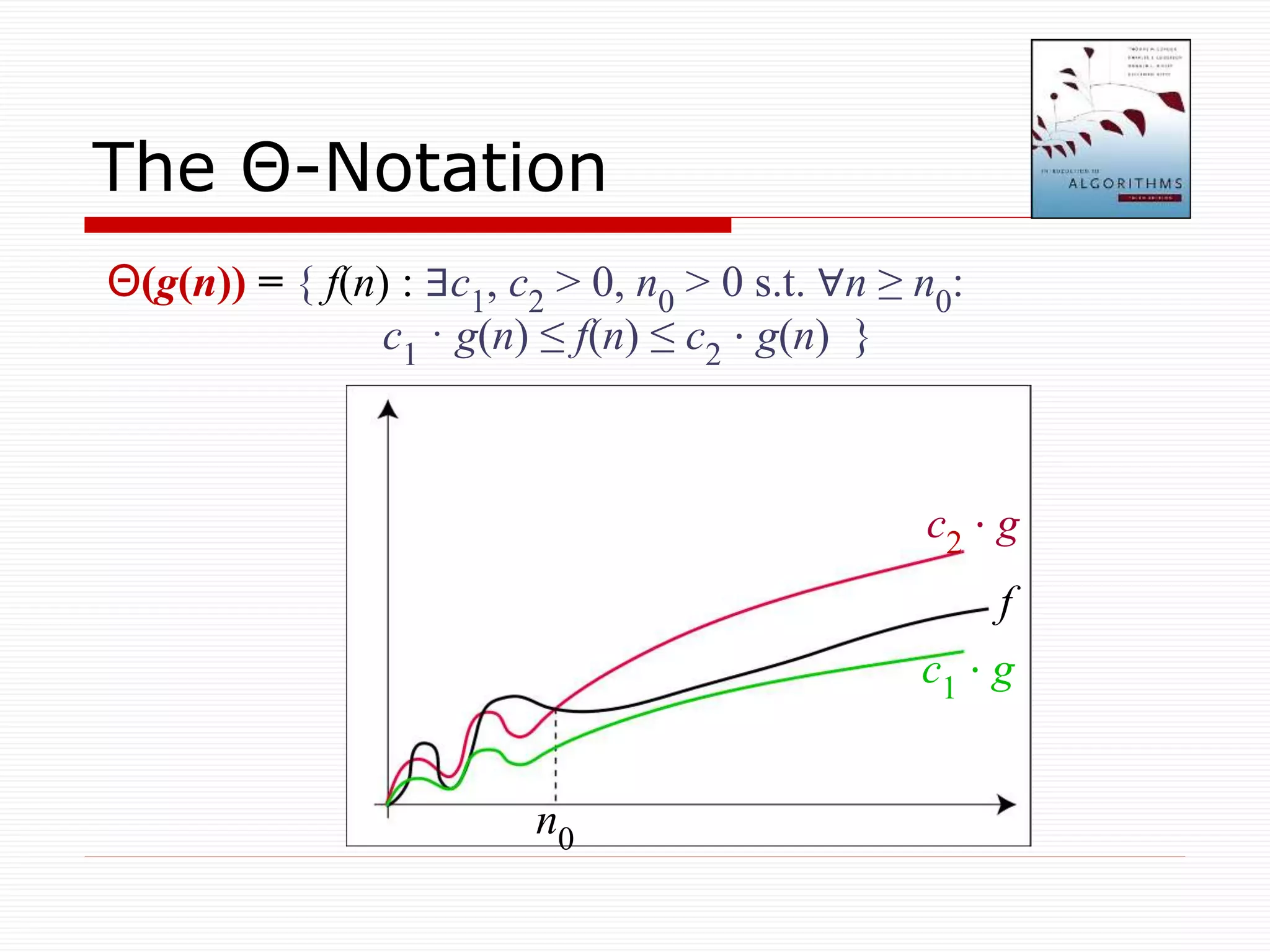
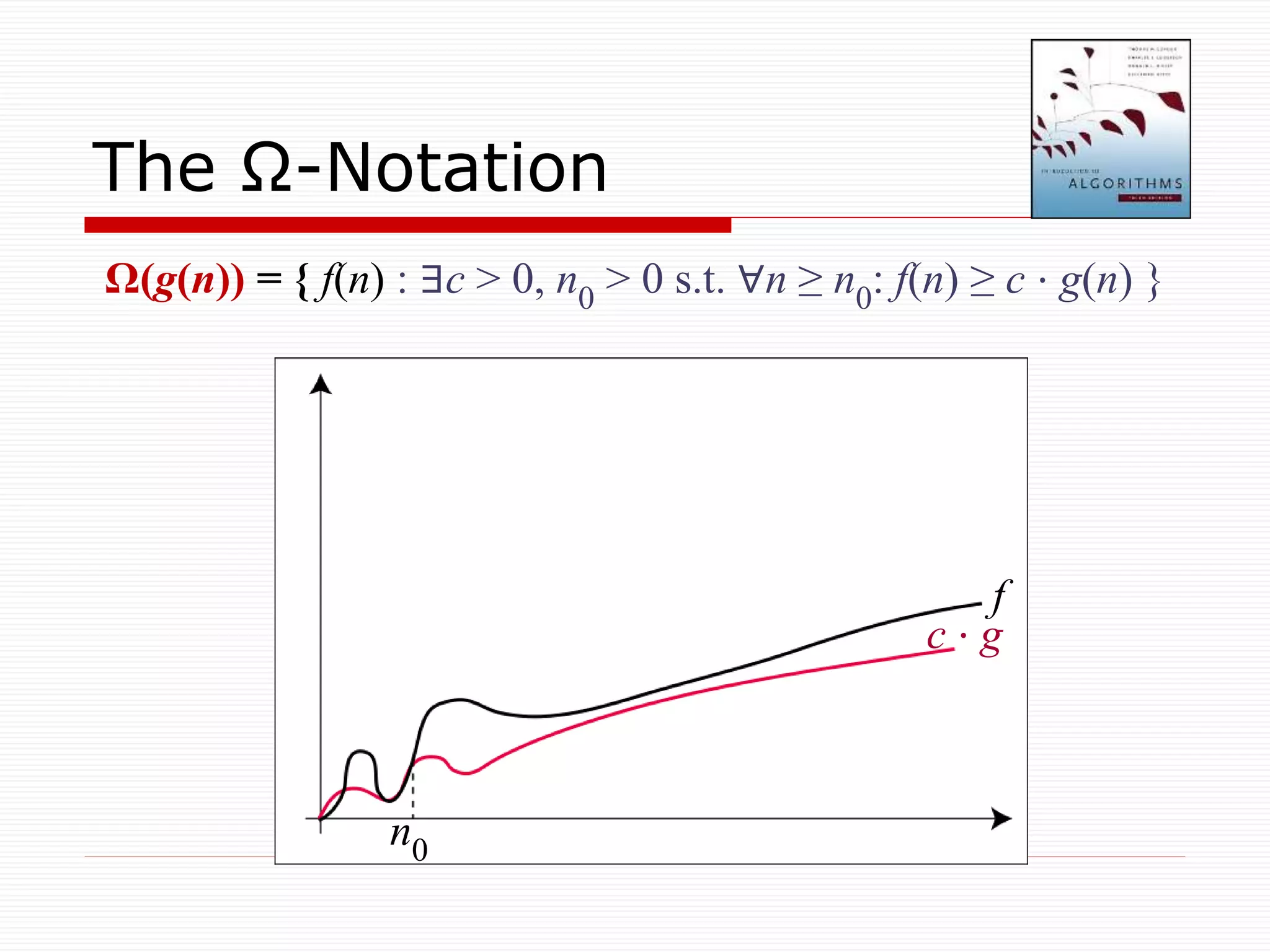
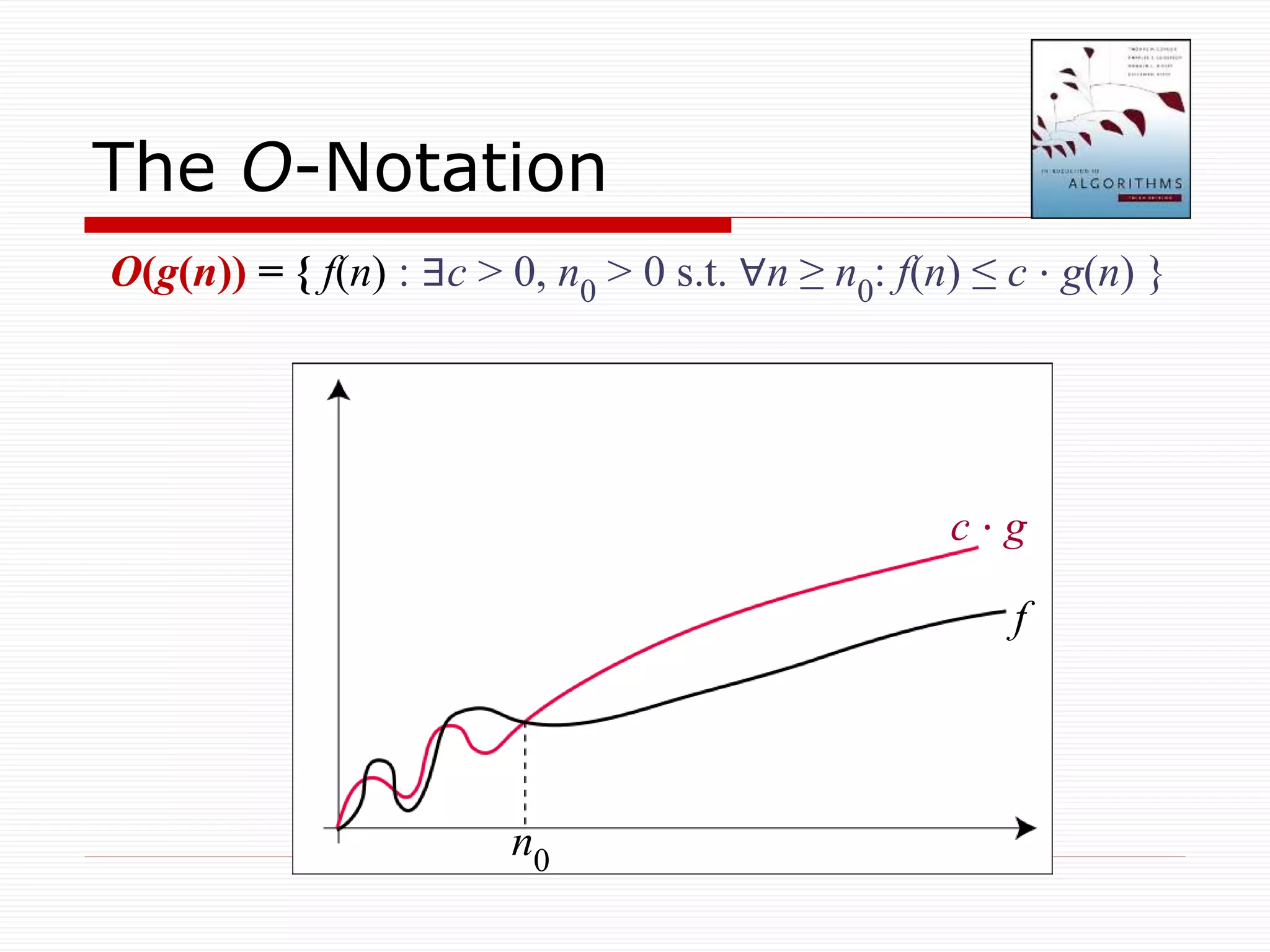
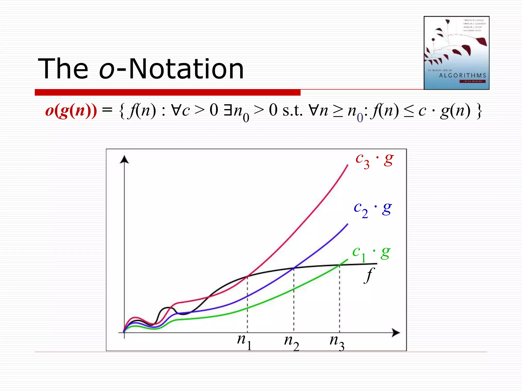
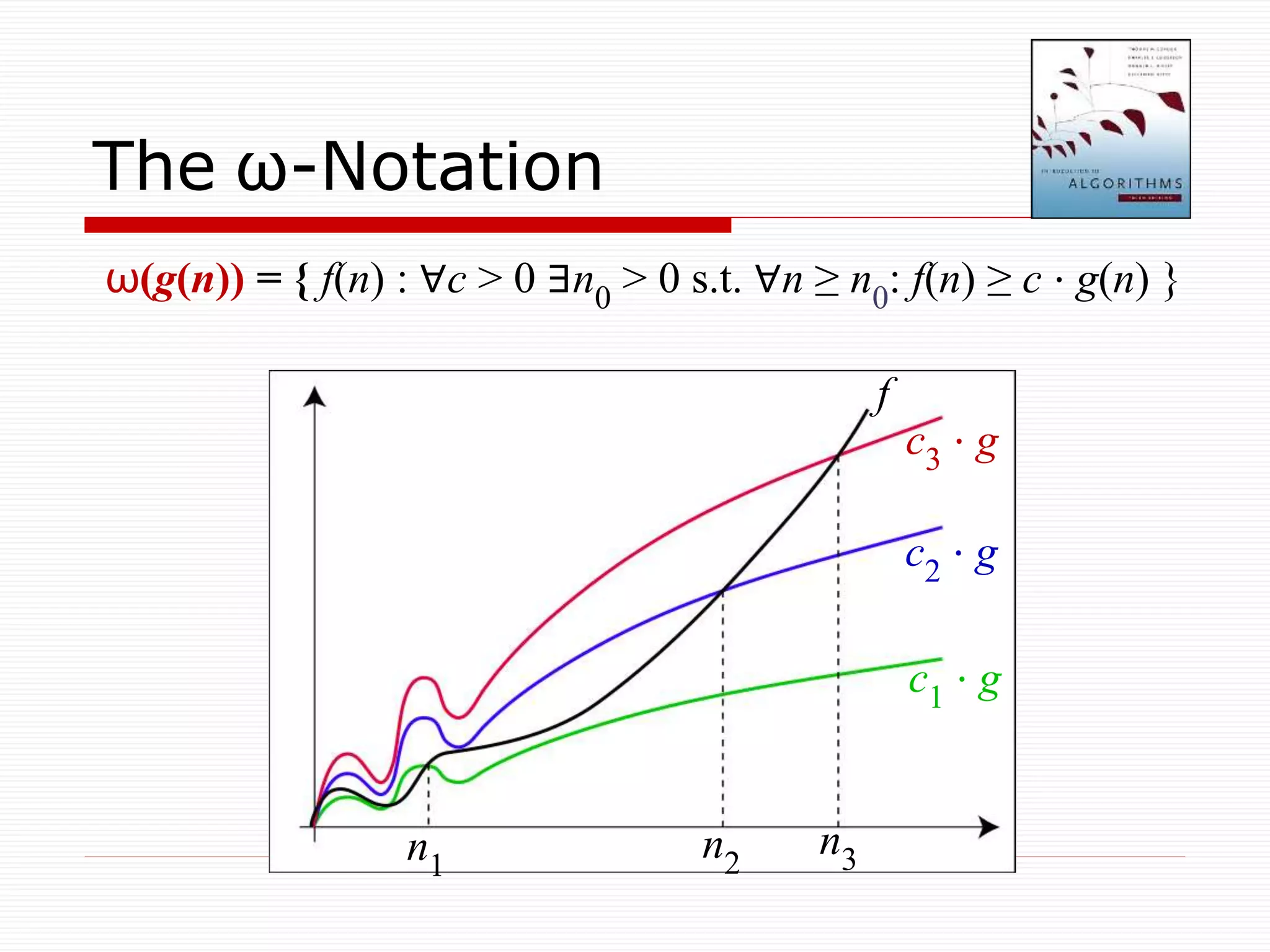
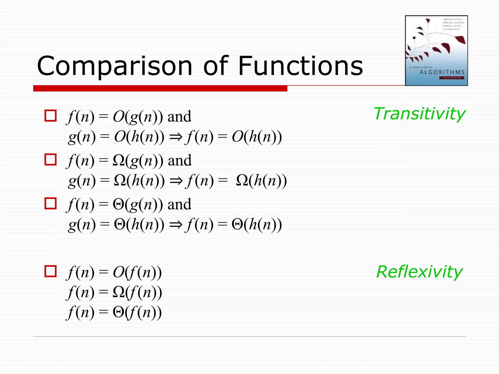
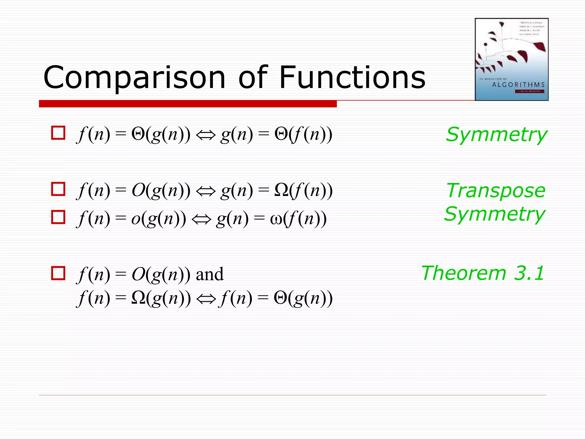
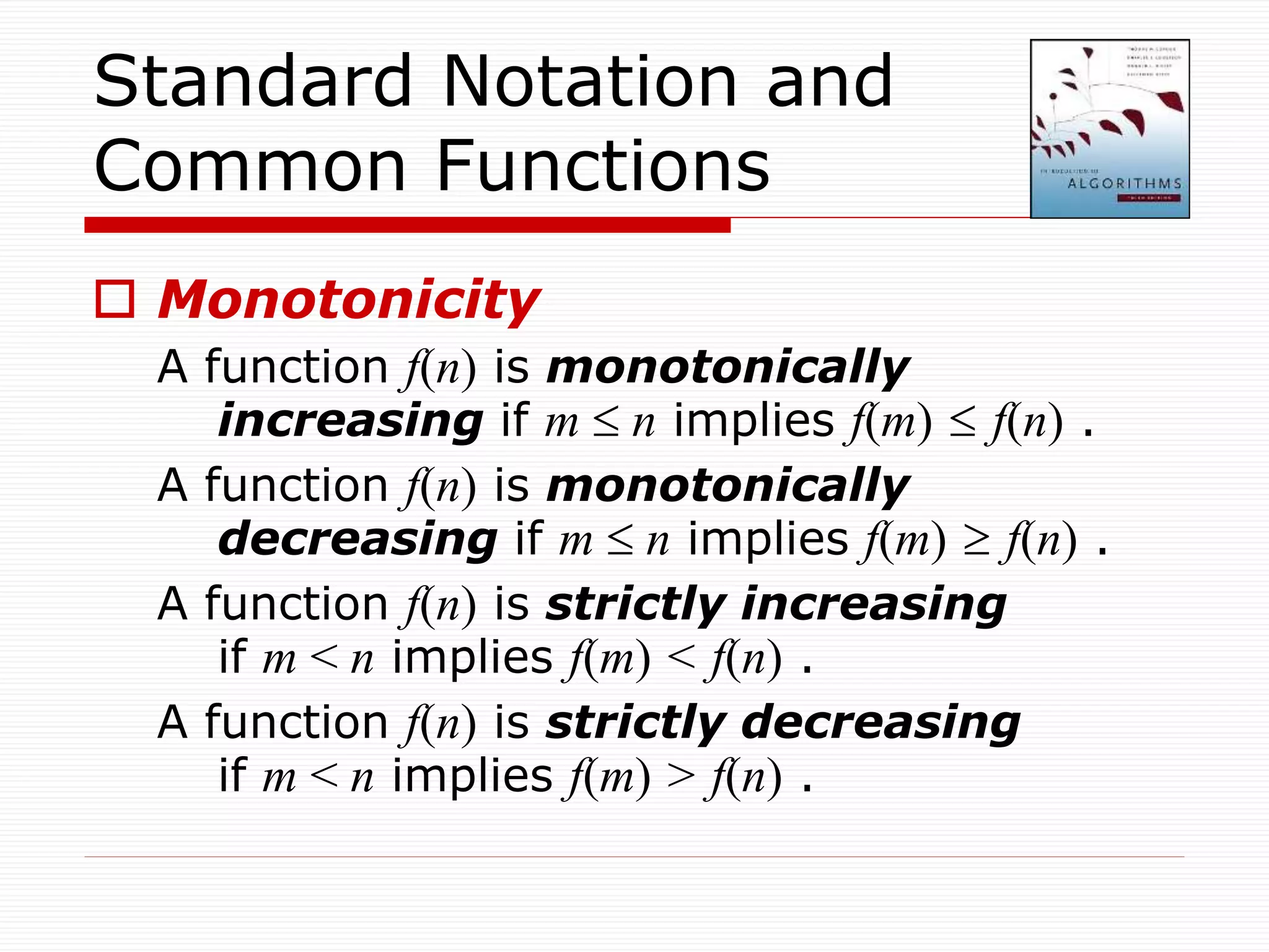
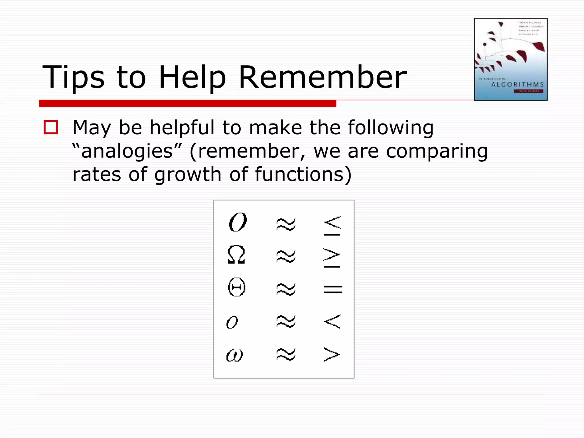
Introduction to Algorithms
(3rd edition)
by Cormen, Leiserson, Rivest & Stein
Chapter 3: Growth of Functions
(slides enhanced by N. Adlai A. DePano)
Overview
 Order of growth of functions provides a
simple characterization of efficiency
 Allows for comparison of relative
performance between alternative
algorithms
 Concerned with asymptotic efficiency of
algorithms
 Best asymptotic efficiency usually is best
choice except for smaller inputs
 Several standard methods to simplify
asymptotic analysis of algorithms
Asymptotic Notation
 Applies to functions whose domains are the
set of natural numbers:
N = {0,1,2,…}
 If time resource T(n) is being analyzed, the
function’s range is usually the set of non-
negative real numbers:
T(n)  R+
 If space resource S(n) is being analyzed, the
function’s range is usually also the set of
natural numbers:
S(n)  N
Asymptotic Notation
 Depending on the textbook,
asymptotic categories may be
expressed in terms of --
a. set membership (our textbook):
functions belong to a family of functions
that exhibit some property; or
b. function property (other textbooks):
functions exhibit the property
 Caveat: we will formally use (a) and
informally use (b)
The Θ-Notation
f
c1 ⋅ g
n0
c2 ⋅ g
Θ(g(n)) = { f(n) : ∃c1, c2 > 0, n0 > 0 s.t. ∀n ≥ n0:
c1 · g(n) ≤ f(n) ≤ c2 ⋅ g(n) }
The Ω-Notation
Ω(g(n)) = { f(n) : ∃c > 0, n0 > 0 s.t. ∀n ≥ n0: f(n) ≥ c ⋅ g(n) }
f
c ⋅ g
n0
The O-Notation
f
c ⋅ g
n0
O(g(n)) = { f(n) : ∃c > 0, n0 > 0 s.t. ∀n ≥ n0: f(n) ≤ c ⋅ g(n) }
The o-Notation
o(g(n)) = { f(n) : ∀c > 0 ∃n0 > 0 s.t. ∀n ≥ n0: f(n) ≤ c ⋅ g(n) }
f
c1 ⋅ g
n1
c2 ⋅ g
c3 ⋅ g
n2 n3
The ω-Notation
f
c1 ⋅ g
n1
c2 ⋅ g
c3 ⋅ g
n2
n3
ω(g(n)) = { f(n) : ∀c > 0 ∃n0 > 0 s.t. ∀n ≥ n0: f(n) ≥ c ⋅ g(n) }
 f(n) = O(g(n)) and
g(n) = O(h(n)) ⇒ f(n) = O(h(n))
 f(n) = Ω(g(n)) and
g(n) = Ω(h(n)) ⇒ f(n) = Ω(h(n))
 f(n) = Θ(g(n)) and
g(n) = Θ(h(n)) ⇒ f(n) = Θ(h(n))
 f(n) = O(f(n))
f(n) = Ω(f(n))
f(n) = Θ(f(n))
Comparison of Functions
Reflexivity
Transitivity
 f (n) = Θ(g(n))  g(n) = Θ(f (n))
 f (n) = O(g(n))  g(n) = Ω(f (n))
 f (n) = o(g(n))  g(n) = ω(f (n))
 f (n) = O(g(n)) and
f (n) = Ω(g(n))  f (n) = Θ(g(n))
Comparison of Functions
Transpose
Symmetry
Symmetry
Theorem 3.1
Standard Notation and
Common Functions
 Monotonicity
A function f(n) is monotonically
increasing if m  n implies f(m)  f(n) .
A function f(n) is monotonically
decreasing if m  n implies f(m)  f(n) .
A function f(n) is strictly increasing
if m < n implies f(m) < f(n) .
A function f(n) is strictly decreasing
if m < n implies f(m) > f(n) .
Standard Notation and
Common Functions
 Floors and ceilings
For any real number x, the greatest integer
less than or equal to x is denoted by x.
For any real number x, the least integer
greater than or equal to x is denoted by
x.
For all real numbers x,
x1 < x  x  x < x+1.
Both functions are monotonically
increasing.
Standard Notation and
Common Functions
 Exponentials
For all n and a1, the function an is the exponential
function with base a and is monotonically
increasing.
 Logarithms
Textbook adopts the following convention
lg n = log2n (binary logarithm),
ln n = logen (natural logarithm),
lgk n = (lg n)k (exponentiation),
lg lg n = lg(lg n) (composition),
lg n + k = (lg n)+k (precedence of lg).
Standard Notation and
Common Functions
 Factorials
For all n the function n! or “n factorial” is
given by
n! = n  (n1)  (n  2)  (n  3)  …  2  1
It can be established that
n! = o(nn)
n! = (2n)
lg(n!) = (nlgn)
 Functional iteration
The notation f (i)(n) represents the function f(n)
iteratively applied i times to an initial value of n,
or, recursively
f (i)(n) = n if i=0
f (i)(n) = f(f (i1)(n)) if i>0
Example:
If f (n) = 2n
then f (2)(n) = f (2n) = 2(2n) = 22n
then f (3)(n) = f (f (2)(n)) = 2(22n) = 23n
then f (i)(n) = 2in
Standard Notation and
Common Functions
 Iterated logarithmic function
The notation lg* n which reads “log star of n” is
defined as
lg* n = min {i0 : lg(i) n  1
Example:
lg* 2 = 1
lg* 4 = 2
lg* 16 = 3
lg* 65536 = 4
lg* 265536 = 5
Standard Notation and
Common Functions
 Asymptotic analysis studies how the
values of functions compare as their
arguments grow without bounds.
 Ignores constants and the behavior of
the function for small arguments.
 Acceptable because all algorithms are
fast for small inputs and growth of
running time is more important than
constant factors.
Things to Remember
 Ignoring the usually unimportant details,
we obtain a representation that succinctly
describes the growth of a function as
its argument grows and thus allows us to
make comparisons between algorithms in
terms of their efficiency.
Things to Remember
Tips to Help Remember
 May be helpful to make the following
“analogies” (remember, we are comparing
rates of growth of functions)

Lecture 4 - Growth of Functions.ppt

  • 1.
    Introduction to Algorithms (3rdedition) by Cormen, Leiserson, Rivest & Stein Chapter 3: Growth of Functions (slides enhanced by N. Adlai A. DePano)
  • 2.
    Overview  Order ofgrowth of functions provides a simple characterization of efficiency  Allows for comparison of relative performance between alternative algorithms  Concerned with asymptotic efficiency of algorithms  Best asymptotic efficiency usually is best choice except for smaller inputs  Several standard methods to simplify asymptotic analysis of algorithms
  • 3.
    Asymptotic Notation  Appliesto functions whose domains are the set of natural numbers: N = {0,1,2,…}  If time resource T(n) is being analyzed, the function’s range is usually the set of non- negative real numbers: T(n)  R+  If space resource S(n) is being analyzed, the function’s range is usually also the set of natural numbers: S(n)  N
  • 4.
    Asymptotic Notation  Dependingon the textbook, asymptotic categories may be expressed in terms of -- a. set membership (our textbook): functions belong to a family of functions that exhibit some property; or b. function property (other textbooks): functions exhibit the property  Caveat: we will formally use (a) and informally use (b)
  • 5.
    The Θ-Notation f c1 ⋅g n0 c2 ⋅ g Θ(g(n)) = { f(n) : ∃c1, c2 > 0, n0 > 0 s.t. ∀n ≥ n0: c1 · g(n) ≤ f(n) ≤ c2 ⋅ g(n) }
  • 6.
    The Ω-Notation Ω(g(n)) ={ f(n) : ∃c > 0, n0 > 0 s.t. ∀n ≥ n0: f(n) ≥ c ⋅ g(n) } f c ⋅ g n0
  • 7.
    The O-Notation f c ⋅g n0 O(g(n)) = { f(n) : ∃c > 0, n0 > 0 s.t. ∀n ≥ n0: f(n) ≤ c ⋅ g(n) }
  • 8.
    The o-Notation o(g(n)) ={ f(n) : ∀c > 0 ∃n0 > 0 s.t. ∀n ≥ n0: f(n) ≤ c ⋅ g(n) } f c1 ⋅ g n1 c2 ⋅ g c3 ⋅ g n2 n3
  • 9.
    The ω-Notation f c1 ⋅g n1 c2 ⋅ g c3 ⋅ g n2 n3 ω(g(n)) = { f(n) : ∀c > 0 ∃n0 > 0 s.t. ∀n ≥ n0: f(n) ≥ c ⋅ g(n) }
  • 10.
     f(n) =O(g(n)) and g(n) = O(h(n)) ⇒ f(n) = O(h(n))  f(n) = Ω(g(n)) and g(n) = Ω(h(n)) ⇒ f(n) = Ω(h(n))  f(n) = Θ(g(n)) and g(n) = Θ(h(n)) ⇒ f(n) = Θ(h(n))  f(n) = O(f(n)) f(n) = Ω(f(n)) f(n) = Θ(f(n)) Comparison of Functions Reflexivity Transitivity
  • 11.
     f (n)= Θ(g(n))  g(n) = Θ(f (n))  f (n) = O(g(n))  g(n) = Ω(f (n))  f (n) = o(g(n))  g(n) = ω(f (n))  f (n) = O(g(n)) and f (n) = Ω(g(n))  f (n) = Θ(g(n)) Comparison of Functions Transpose Symmetry Symmetry Theorem 3.1
  • 12.
    Standard Notation and CommonFunctions  Monotonicity A function f(n) is monotonically increasing if m  n implies f(m)  f(n) . A function f(n) is monotonically decreasing if m  n implies f(m)  f(n) . A function f(n) is strictly increasing if m < n implies f(m) < f(n) . A function f(n) is strictly decreasing if m < n implies f(m) > f(n) .
  • 13.
    Standard Notation and CommonFunctions  Floors and ceilings For any real number x, the greatest integer less than or equal to x is denoted by x. For any real number x, the least integer greater than or equal to x is denoted by x. For all real numbers x, x1 < x  x  x < x+1. Both functions are monotonically increasing.
  • 14.
    Standard Notation and CommonFunctions  Exponentials For all n and a1, the function an is the exponential function with base a and is monotonically increasing.  Logarithms Textbook adopts the following convention lg n = log2n (binary logarithm), ln n = logen (natural logarithm), lgk n = (lg n)k (exponentiation), lg lg n = lg(lg n) (composition), lg n + k = (lg n)+k (precedence of lg).
  • 15.
    Standard Notation and CommonFunctions  Factorials For all n the function n! or “n factorial” is given by n! = n  (n1)  (n  2)  (n  3)  …  2  1 It can be established that n! = o(nn) n! = (2n) lg(n!) = (nlgn)
  • 16.
     Functional iteration Thenotation f (i)(n) represents the function f(n) iteratively applied i times to an initial value of n, or, recursively f (i)(n) = n if i=0 f (i)(n) = f(f (i1)(n)) if i>0 Example: If f (n) = 2n then f (2)(n) = f (2n) = 2(2n) = 22n then f (3)(n) = f (f (2)(n)) = 2(22n) = 23n then f (i)(n) = 2in Standard Notation and Common Functions
  • 17.
     Iterated logarithmicfunction The notation lg* n which reads “log star of n” is defined as lg* n = min {i0 : lg(i) n  1 Example: lg* 2 = 1 lg* 4 = 2 lg* 16 = 3 lg* 65536 = 4 lg* 265536 = 5 Standard Notation and Common Functions
  • 18.
     Asymptotic analysisstudies how the values of functions compare as their arguments grow without bounds.  Ignores constants and the behavior of the function for small arguments.  Acceptable because all algorithms are fast for small inputs and growth of running time is more important than constant factors. Things to Remember
  • 19.
     Ignoring theusually unimportant details, we obtain a representation that succinctly describes the growth of a function as its argument grows and thus allows us to make comparisons between algorithms in terms of their efficiency. Things to Remember
  • 20.
    Tips to HelpRemember  May be helpful to make the following “analogies” (remember, we are comparing rates of growth of functions)