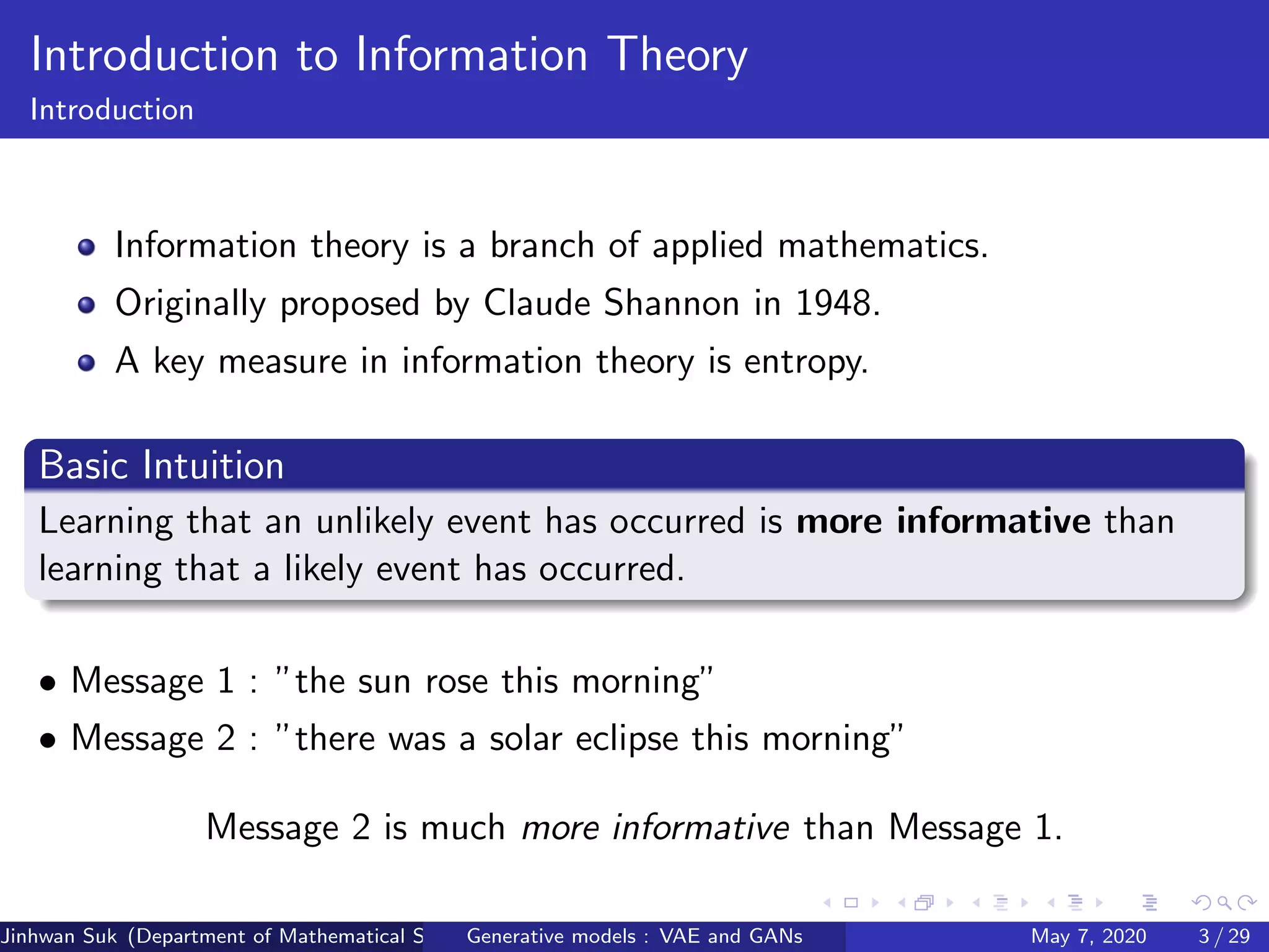
This document summarizes generative models like VAEs and GANs. It begins with an introduction to information theory, defining key concepts like entropy and maximum likelihood estimation. It then explains generative models as estimating the joint distribution P(X,Y) compared to discriminative models estimating P(Y|X). VAEs are discussed as maximizing the evidence lower bound (ELBO) to estimate the latent variable distribution P(Z|X), allowing generation of new X values. GANs are also covered, defining their minimax game between a generator G and discriminator D, with G learning to generate samples resembling the real data distribution Pemp.
![Introduction to Information Theory
Measure of Information
Definition (Self-Informaiton)
self-information of an event X = x is
I(x) = − log P(x).
self-information is a measure of information(or, uncertainity, surprise) of a
certain single event.
Definition (Shannon-Entropy)
Shannon entropy is the expected amount of information in an entire
probability distribution defined by
H(X) = EX∼P[I(X)] = −EX∼P[log P(X)].
Jinhwan Suk (Department of Mathematical Science, KAIST)Generative models : VAE and GANs May 7, 2020 6 / 29](https://image.slidesharecdn.com/gm-200507144033/75/Generative-models-VAE-and-GAN-6-2048.jpg)
![Introduction to Information Theory
Density Estimation
In classification problem, we usually want to describe P(Y |X) for
each input X.
So many models(cθ) aim to estimate conditional probability
distribution by choosing optimal ˆθ such that
cˆθ(x)[i] = P(Y = yi |X = x),
like softmax classifier or Logistic regresor.
So we can regard the classification problem as the regression problem
such that minimizes
R(cθ) = EX [L(cθ(X), P(Y |X))]
(L measures distance between two probability distribution)
Jinhwan Suk (Department of Mathematical Science, KAIST)Generative models : VAE and GANs May 7, 2020 7 / 29](https://image.slidesharecdn.com/gm-200507144033/75/Generative-models-VAE-and-GAN-7-2048.jpg)
![Introduction to Information Theory
Two ways of measuring distance between probability distributions
Definition (Total variation)
The total variation distance between two probability measures Pθ and
Pθ∗ is defined by
TV (Pθ, Pθ∗ ) = max
A:events
|Pθ(A) − Pθ∗ (A)|.
Definition (Kullback-Leibler divergence)
The KL divergence between two probability measures Pθ and Pθ∗ is
defined by
DKL(Pθ||Pθ∗ ) = EX∼Pθ
[log Pθ(X) − log Pθ∗ (X)],
Jinhwan Suk (Department of Mathematical Science, KAIST)Generative models : VAE and GANs May 7, 2020 8 / 29](https://image.slidesharecdn.com/gm-200507144033/75/Generative-models-VAE-and-GAN-8-2048.jpg)
![Introduction to Information Theory
Cross-Entropy
We usually use KL-divergence because finding estimator of θ is much
easier in KL-divergence.
DKL(Pθ||Pθ∗ ) = EX∼Pθ
[log P(X) − log Pθ∗ (X)]
= EX∼Pθ
[log Pθ(X)] − EX∼Pθ
[log Pθ∗ (X)]
= constant − EX∼Pθ
[log Pθ∗ (X)]
Hence, minimizing the KL divergence is equivalent to minimizing
−EX∼Pθ
[log Pθ∗ (x)], whose name is cross-entropy. And the estimation
using estimator that minimizes KL divergence or Cross-entropy is called
maximum likelihood principle.
Jinhwan Suk (Department of Mathematical Science, KAIST)Generative models : VAE and GANs May 7, 2020 9 / 29](https://image.slidesharecdn.com/gm-200507144033/75/Generative-models-VAE-and-GAN-9-2048.jpg)
![Introduction to Information Theory
Maximum Likelihood Estimation
Pθ∗ is distribution of population and we want to choose proper estimator ˆθ
by minimizing the distance between Pθ∗ and Pˆθ,
DKL(Pθ∗ || Pˆθ) = const − EX∼Pθ∗ [log Pˆθ(X)]
If X1, X2, ..., Xn are random samples, then by LLN,
EX∼Pθ∗ [log Pˆθ(x)] ∼
1
n
n
i=1
log Pˆθ(Xi )
∴ DKL(Pθ∗ || Pˆθ) = const −
1
n
n
i=1
log Pˆθ(Xi )
Jinhwan Suk (Department of Mathematical Science, KAIST)Generative models : VAE and GANs May 7, 2020 10 / 29](https://image.slidesharecdn.com/gm-200507144033/75/Generative-models-VAE-and-GAN-10-2048.jpg)
![Introduction to Information Theory
Return to Main Goal : Find an estimator ˆθ that minimizes
R(cθ) = EX [L(cθ(X), P(Y |X))].
Suppose that X1, X2, ..., Xn are i.i.d and cross-entropy is used for L.
EX [L(cθ(X), P(Y |X))] ∼
1
n
n
i=1
L(cθ(Xi ), P(Y |Xi ))
=
1
n
n
i=1
−EY |Xi ∼PYemp|Xi
[log cθ(Xi )]
=
1
n
n
i=1
− log{cθ(Xi )[Yi,true]}.
Jinhwan Suk (Department of Mathematical Science, KAIST)Generative models : VAE and GANs May 7, 2020 12 / 29](https://image.slidesharecdn.com/gm-200507144033/75/Generative-models-VAE-and-GAN-12-2048.jpg)
![Concept of VAE
Goal : estimate population distribution using given observations.
Strong assumption on existence of latent variables, Z ∼ N(0, I).
X|Z ∼ N(f (Z; θ), σ2
∗ I))
X|Z ∼ Bernoulli(f (Z; θ))
Let Pemp be empirical distribution(assumption : Pemp ≈ Ppop)
arg min
θ
DKL(Pemp(X)||Pθ(X)) = arg min
θ
const − EX∼Pemp [log Pθ(X)]
= arg max
θ
EX∼Pemp [log Pθ(X)]
= arg max
θ
1
N
N
i=1
[log Pθ(Xi )]
Jinhwan Suk (Department of Mathematical Science, KAIST)Generative models : VAE and GANs May 7, 2020 15 / 29](https://image.slidesharecdn.com/gm-200507144033/75/Generative-models-VAE-and-GAN-15-2048.jpg)
![Concept of VAE
DKL(Qφ(Z|X)||Pθ(Z|X)) = EZ∼Q|X [log Qφ(Z|X) − log Pθ(Z|X)]
= EZ∼Q|X [log Qφ(Z|X) − log Pθ(X, Z)]
+ log Pθ(X)
We want to maximize log Pθ(X) and minimize
DKL(Qφ(Z|X)||Pθ(Z|X)) at once.
Define L(θ, φ, X) = EZ∼Q|X [log Pθ(X, Z) − log Qφ(Z|X)]
log Pθ(X) − DKL(Qφ(Z|X)||Pθ(Z|X)) = L(θ, φ, X)
Jinhwan Suk (Department of Mathematical Science, KAIST)Generative models : VAE and GANs May 7, 2020 18 / 29](https://image.slidesharecdn.com/gm-200507144033/75/Generative-models-VAE-and-GAN-18-2048.jpg)
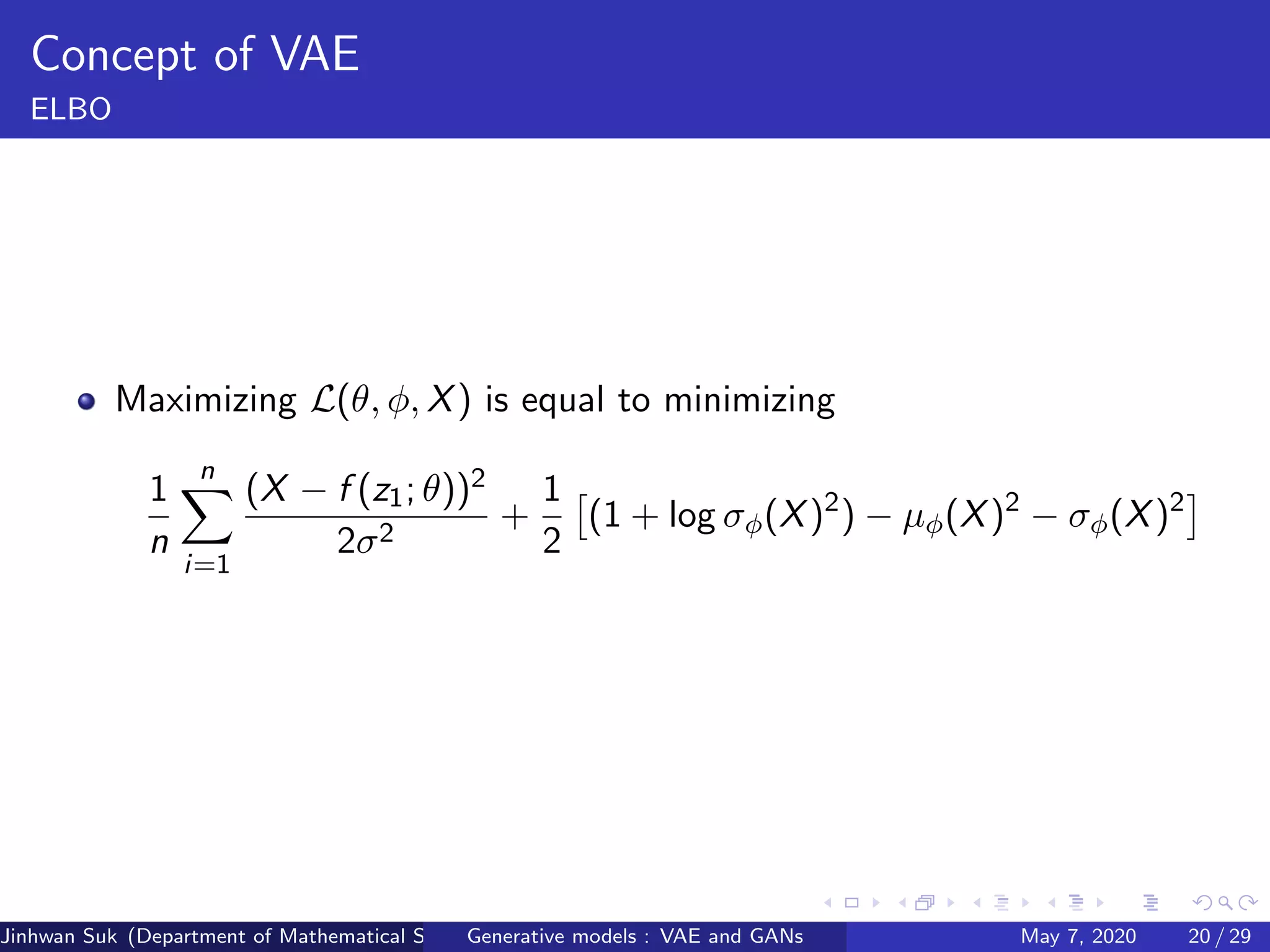
![Concept of VAE
ELBO
L(θ, φ, X) = EZ∼Q|X [log Pθ(X, Z) − log Qφ(Z|X)]
= EZ∼Q|X [log Pθ(X|Z) + log Pθ(Z) − log Qφ(Z|X)]
= EZ∼Q|X [log Pθ(X|Z)] − DKL(Qφ(Z|X)||Pθ(Z))
DKL(Qφ(Z|X)||Pθ(Z)) can be integrated analytically
DKL(Qφ(Z|X)||Pθ(Z)) =
1
2
(1 + log σφ(X)2
) − µφ(X)2
− σφ(X)2
EZ∼Q|X [log Pθ(X|Z)] requires estimation by sampling.
EZ∼Q|X [log Pθ(X|Z)] ≈
1
n
n
i=1
log Pθ(X|zi )
=
1
n
n
i=1
[−
(X − f (z1; θ))2
2σ2
− log(
√
2πσ2
)]
Jinhwan Suk (Department of Mathematical Science, KAIST)Generative models : VAE and GANs May 7, 2020 19 / 29](https://image.slidesharecdn.com/gm-200507144033/75/Generative-models-VAE-and-GAN-19-2048.jpg)
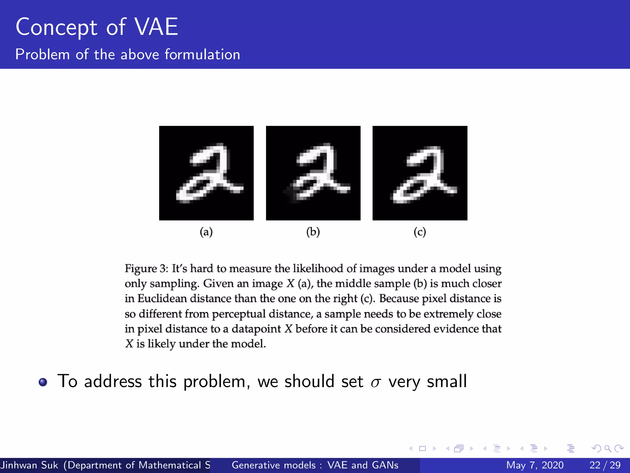
![Concept of VAE
Problem of the above formulation
Since Pθ(Xi ) ≈ 1
n
n
j=1 P(Xi |zj )P(zj ) and we use n = 1,
log Pθ(Xi ) ≈ log[P(Xi |z1)P(z1)]
= log P(Xi |z1) + log P(z1)
= log
1
√
2πσ
exp(−
(Xi − f (z1; θ))2
2σ2
) + log
1
√
2π
exp(−
z2
1
2
)
= −
(Xi − f (z1; θ))2
2σ2
+ const.
Therfore, maximizing log Pθ(Xi ) is transformed to
minimizing −(Xi −f (z1;θ))2
2σ2 .
Jinhwan Suk (Department of Mathematical Science, KAIST)Generative models : VAE and GANs May 7, 2020 21 / 29](https://image.slidesharecdn.com/gm-200507144033/75/Generative-models-VAE-and-GAN-21-2048.jpg)
![Concept of GANs
Introduction
Goal : estimate population distribution using given observations.
Strong assumption on existence of latent variables, Z ∼ PZ .
Define G(z; θg ) which is mapping to data space,
Pg (X = x) = PZ (G(Z) = x)
Define D(x; θd ) that represents the probability that x is real.
min
G
max
D
V (D, G) = Ex∼Pemp [log D(x)] + E[log(1 − D(G(z)))]
What is difference between VAE and GANs??
⇒ GANs do not formulate about P(X) explicitly.
⇒ But we can show it has a global optimum Pg = Pemp
⇒ So we can say that GANs is generative model.
Jinhwan Suk (Department of Mathematical Science, KAIST)Generative models : VAE and GANs May 7, 2020 23 / 29](https://image.slidesharecdn.com/gm-200507144033/75/Generative-models-VAE-and-GAN-23-2048.jpg)
![Concept of GANs
Algorithm
V (D, G) = Ex∼Pemp [log D(x)] + E[log(1 − D(G(z)))]
∼
1
m
m
i=1
log D(xi ) +
1
m
m
j=1
log(1 − D(G(zj )))
1 Sample minibatch of m noise samples and minibatch of m examples.
2 update the discriminator by ascending its stochastic gradient :
1
m
m
i=1
θd
[log D(xi ) + log(1 − D(G(zi )))]
3 Sample minibatch of m noise samples.
4 Update the generator by descending its stochastic gradient :
1
m
m
i=1
θg [log(1 − D(G(zi )))]
Jinhwan Suk (Department of Mathematical Science, KAIST)Generative models : VAE and GANs May 7, 2020 24 / 29](https://image.slidesharecdn.com/gm-200507144033/75/Generative-models-VAE-and-GAN-24-2048.jpg)
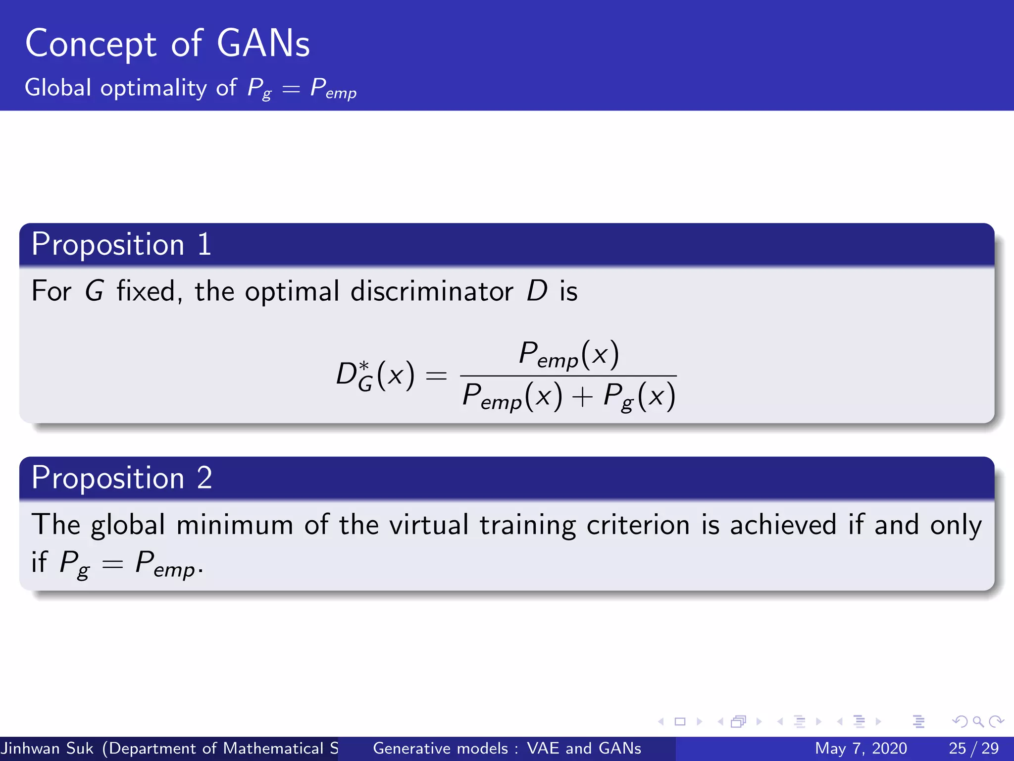

![proof of Proposition 1(continued) :
V (G, Dθ) achieves the minimum when
∂
∂θ [log(Dθ(x))Pemp(x) + log(1 − Dθ(x))Pg (x)] = 0 ∀x ∈ X.
⇔
∂
∂θ
Dθ(x)
Dθ(x) Pemp(x) −
∂
∂θ
Dθ(x)
1−Dθ(x) Pg (x) = 0 ∀x ∈ X
⇔ Dˆθ(x) =
Pemp(x)
Pemp(x)+Pg (x) ∀x ∈ X
Jinhwan Suk (Department of Mathematical Science, KAIST)Generative models : VAE and GANs May 7, 2020 27 / 29](https://image.slidesharecdn.com/gm-200507144033/75/Generative-models-VAE-and-GAN-27-2048.jpg)
![proof of Proposition 2 :
min
G
max
D
V (G, D) = min
G
V (G, D∗
G )
= Ex∼Pemp
[log D∗
G (x)] + E[log(1 − D∗
G (G(z)))]
= Ex∼Pemp
[log D∗
G (x)] + Ex∼Pg
[log(1 − D∗
G (x))]
= Ex∼Pemp
log
Pemp(x)
Pemp(x) + Pg (x)
+ Ex∼Pg
log
Pg (x)
Pemp(x) + Pg (x)
= Ex∼Pemp
log Pemp(x) − log
Pemp(x) + Pg (x)
2
− log 2
+ Ex∼Pg log Pg (x) − log
Pemp(x) + Pg (x)
2
− log 2
= DKL(Pemp||
Pemp(x) + Pg (x)
2
) + DKL(Pg ||
Pemp(x) + Pg (x)
2
)
− 2 log 2
≥ −2 log 2
The equality holds if and only if Pemp =
Pemp(x)+Pg (x)
2 and Pg =
Pemp(x)+Pg (x)
2
Jinhwan Suk (Department of Mathematical Science, KAIST)Generative models : VAE and GANs May 7, 2020 28 / 29](https://image.slidesharecdn.com/gm-200507144033/75/Generative-models-VAE-and-GAN-28-2048.jpg)


![Introduction to Information Theory
Measure of Information
Definition (Self-Informaiton)
self-information of an event X = x is
I(x) = − log P(x).
self-information is a measure of information(or, uncertainity, surprise) of a
certain single event.
Definition (Shannon-Entropy)
Shannon entropy is the expected amount of information in an entire
probability distribution defined by
H(X) = EX∼P[I(X)] = −EX∼P[log P(X)].
Jinhwan Suk (Department of Mathematical Science, KAIST)Generative models : VAE and GANs May 7, 2020 6 / 29](https://crownmelresort.com/image.slidesharecdn.com/gm-200507144033/75/Generative-models-VAE-and-GAN-6-2048.jpg)
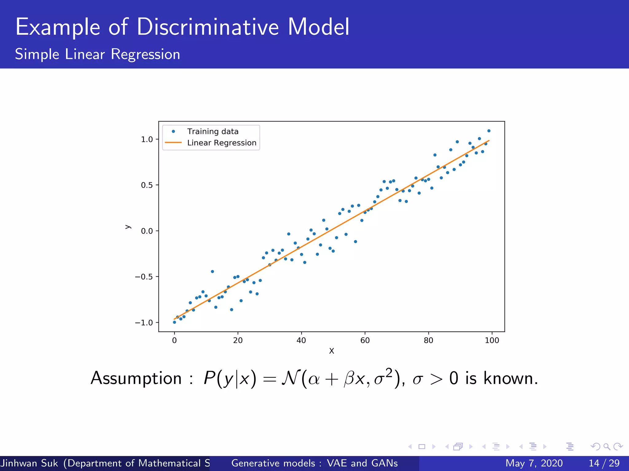
![Introduction to Information Theory
Density Estimation
In classification problem, we usually want to describe P(Y |X) for
each input X.
So many models(cθ) aim to estimate conditional probability
distribution by choosing optimal ˆθ such that
cˆθ(x)[i] = P(Y = yi |X = x),
like softmax classifier or Logistic regresor.
So we can regard the classification problem as the regression problem
such that minimizes
R(cθ) = EX [L(cθ(X), P(Y |X))]
(L measures distance between two probability distribution)
Jinhwan Suk (Department of Mathematical Science, KAIST)Generative models : VAE and GANs May 7, 2020 7 / 29](https://crownmelresort.com/image.slidesharecdn.com/gm-200507144033/75/Generative-models-VAE-and-GAN-7-2048.jpg)
![Introduction to Information Theory
Two ways of measuring distance between probability distributions
Definition (Total variation)
The total variation distance between two probability measures Pθ and
Pθ∗ is defined by
TV (Pθ, Pθ∗ ) = max
A:events
|Pθ(A) − Pθ∗ (A)|.
Definition (Kullback-Leibler divergence)
The KL divergence between two probability measures Pθ and Pθ∗ is
defined by
DKL(Pθ||Pθ∗ ) = EX∼Pθ
[log Pθ(X) − log Pθ∗ (X)],
Jinhwan Suk (Department of Mathematical Science, KAIST)Generative models : VAE and GANs May 7, 2020 8 / 29](https://crownmelresort.com/image.slidesharecdn.com/gm-200507144033/75/Generative-models-VAE-and-GAN-8-2048.jpg)
![Introduction to Information Theory
Cross-Entropy
We usually use KL-divergence because finding estimator of θ is much
easier in KL-divergence.
DKL(Pθ||Pθ∗ ) = EX∼Pθ
[log P(X) − log Pθ∗ (X)]
= EX∼Pθ
[log Pθ(X)] − EX∼Pθ
[log Pθ∗ (X)]
= constant − EX∼Pθ
[log Pθ∗ (X)]
Hence, minimizing the KL divergence is equivalent to minimizing
−EX∼Pθ
[log Pθ∗ (x)], whose name is cross-entropy. And the estimation
using estimator that minimizes KL divergence or Cross-entropy is called
maximum likelihood principle.
Jinhwan Suk (Department of Mathematical Science, KAIST)Generative models : VAE and GANs May 7, 2020 9 / 29](https://crownmelresort.com/image.slidesharecdn.com/gm-200507144033/75/Generative-models-VAE-and-GAN-9-2048.jpg)
![Introduction to Information Theory
Maximum Likelihood Estimation
Pθ∗ is distribution of population and we want to choose proper estimator ˆθ
by minimizing the distance between Pθ∗ and Pˆθ,
DKL(Pθ∗ || Pˆθ) = const − EX∼Pθ∗ [log Pˆθ(X)]
If X1, X2, ..., Xn are random samples, then by LLN,
EX∼Pθ∗ [log Pˆθ(x)] ∼
1
n
n
i=1
log Pˆθ(Xi )
∴ DKL(Pθ∗ || Pˆθ) = const −
1
n
n
i=1
log Pˆθ(Xi )
Jinhwan Suk (Department of Mathematical Science, KAIST)Generative models : VAE and GANs May 7, 2020 10 / 29](https://crownmelresort.com/image.slidesharecdn.com/gm-200507144033/75/Generative-models-VAE-and-GAN-10-2048.jpg)

![Introduction to Information Theory
Return to Main Goal : Find an estimator ˆθ that minimizes
R(cθ) = EX [L(cθ(X), P(Y |X))].
Suppose that X1, X2, ..., Xn are i.i.d and cross-entropy is used for L.
EX [L(cθ(X), P(Y |X))] ∼
1
n
n
i=1
L(cθ(Xi ), P(Y |Xi ))
=
1
n
n
i=1
−EY |Xi ∼PYemp|Xi
[log cθ(Xi )]
=
1
n
n
i=1
− log{cθ(Xi )[Yi,true]}.
Jinhwan Suk (Department of Mathematical Science, KAIST)Generative models : VAE and GANs May 7, 2020 12 / 29](https://crownmelresort.com/image.slidesharecdn.com/gm-200507144033/75/Generative-models-VAE-and-GAN-12-2048.jpg)


![Concept of VAE
Goal : estimate population distribution using given observations.
Strong assumption on existence of latent variables, Z ∼ N(0, I).
X|Z ∼ N(f (Z; θ), σ2
∗ I))
X|Z ∼ Bernoulli(f (Z; θ))
Let Pemp be empirical distribution(assumption : Pemp ≈ Ppop)
arg min
θ
DKL(Pemp(X)||Pθ(X)) = arg min
θ
const − EX∼Pemp [log Pθ(X)]
= arg max
θ
EX∼Pemp [log Pθ(X)]
= arg max
θ
1
N
N
i=1
[log Pθ(Xi )]
Jinhwan Suk (Department of Mathematical Science, KAIST)Generative models : VAE and GANs May 7, 2020 15 / 29](https://crownmelresort.com/image.slidesharecdn.com/gm-200507144033/75/Generative-models-VAE-and-GAN-15-2048.jpg)


![Concept of VAE
DKL(Qφ(Z|X)||Pθ(Z|X)) = EZ∼Q|X [log Qφ(Z|X) − log Pθ(Z|X)]
= EZ∼Q|X [log Qφ(Z|X) − log Pθ(X, Z)]
+ log Pθ(X)
We want to maximize log Pθ(X) and minimize
DKL(Qφ(Z|X)||Pθ(Z|X)) at once.
Define L(θ, φ, X) = EZ∼Q|X [log Pθ(X, Z) − log Qφ(Z|X)]
log Pθ(X) − DKL(Qφ(Z|X)||Pθ(Z|X)) = L(θ, φ, X)
Jinhwan Suk (Department of Mathematical Science, KAIST)Generative models : VAE and GANs May 7, 2020 18 / 29](https://crownmelresort.com/image.slidesharecdn.com/gm-200507144033/75/Generative-models-VAE-and-GAN-18-2048.jpg)
![Concept of VAE
ELBO
L(θ, φ, X) = EZ∼Q|X [log Pθ(X, Z) − log Qφ(Z|X)]
= EZ∼Q|X [log Pθ(X|Z) + log Pθ(Z) − log Qφ(Z|X)]
= EZ∼Q|X [log Pθ(X|Z)] − DKL(Qφ(Z|X)||Pθ(Z))
DKL(Qφ(Z|X)||Pθ(Z)) can be integrated analytically
DKL(Qφ(Z|X)||Pθ(Z)) =
1
2
(1 + log σφ(X)2
) − µφ(X)2
− σφ(X)2
EZ∼Q|X [log Pθ(X|Z)] requires estimation by sampling.
EZ∼Q|X [log Pθ(X|Z)] ≈
1
n
n
i=1
log Pθ(X|zi )
=
1
n
n
i=1
[−
(X − f (z1; θ))2
2σ2
− log(
√
2πσ2
)]
Jinhwan Suk (Department of Mathematical Science, KAIST)Generative models : VAE and GANs May 7, 2020 19 / 29](https://crownmelresort.com/image.slidesharecdn.com/gm-200507144033/75/Generative-models-VAE-and-GAN-19-2048.jpg)

![Concept of VAE
Problem of the above formulation
Since Pθ(Xi ) ≈ 1
n
n
j=1 P(Xi |zj )P(zj ) and we use n = 1,
log Pθ(Xi ) ≈ log[P(Xi |z1)P(z1)]
= log P(Xi |z1) + log P(z1)
= log
1
√
2πσ
exp(−
(Xi − f (z1; θ))2
2σ2
) + log
1
√
2π
exp(−
z2
1
2
)
= −
(Xi − f (z1; θ))2
2σ2
+ const.
Therfore, maximizing log Pθ(Xi ) is transformed to
minimizing −(Xi −f (z1;θ))2
2σ2 .
Jinhwan Suk (Department of Mathematical Science, KAIST)Generative models : VAE and GANs May 7, 2020 21 / 29](https://crownmelresort.com/image.slidesharecdn.com/gm-200507144033/75/Generative-models-VAE-and-GAN-21-2048.jpg)

![Concept of GANs
Introduction
Goal : estimate population distribution using given observations.
Strong assumption on existence of latent variables, Z ∼ PZ .
Define G(z; θg ) which is mapping to data space,
Pg (X = x) = PZ (G(Z) = x)
Define D(x; θd ) that represents the probability that x is real.
min
G
max
D
V (D, G) = Ex∼Pemp [log D(x)] + E[log(1 − D(G(z)))]
What is difference between VAE and GANs??
⇒ GANs do not formulate about P(X) explicitly.
⇒ But we can show it has a global optimum Pg = Pemp
⇒ So we can say that GANs is generative model.
Jinhwan Suk (Department of Mathematical Science, KAIST)Generative models : VAE and GANs May 7, 2020 23 / 29](https://crownmelresort.com/image.slidesharecdn.com/gm-200507144033/75/Generative-models-VAE-and-GAN-23-2048.jpg)
![Concept of GANs
Algorithm
V (D, G) = Ex∼Pemp [log D(x)] + E[log(1 − D(G(z)))]
∼
1
m
m
i=1
log D(xi ) +
1
m
m
j=1
log(1 − D(G(zj )))
1 Sample minibatch of m noise samples and minibatch of m examples.
2 update the discriminator by ascending its stochastic gradient :
1
m
m
i=1
θd
[log D(xi ) + log(1 − D(G(zi )))]
3 Sample minibatch of m noise samples.
4 Update the generator by descending its stochastic gradient :
1
m
m
i=1
θg [log(1 − D(G(zi )))]
Jinhwan Suk (Department of Mathematical Science, KAIST)Generative models : VAE and GANs May 7, 2020 24 / 29](https://crownmelresort.com/image.slidesharecdn.com/gm-200507144033/75/Generative-models-VAE-and-GAN-24-2048.jpg)


![proof of Proposition 1(continued) :
V (G, Dθ) achieves the minimum when
∂
∂θ [log(Dθ(x))Pemp(x) + log(1 − Dθ(x))Pg (x)] = 0 ∀x ∈ X.
⇔
∂
∂θ
Dθ(x)
Dθ(x) Pemp(x) −
∂
∂θ
Dθ(x)
1−Dθ(x) Pg (x) = 0 ∀x ∈ X
⇔ Dˆθ(x) =
Pemp(x)
Pemp(x)+Pg (x) ∀x ∈ X
Jinhwan Suk (Department of Mathematical Science, KAIST)Generative models : VAE and GANs May 7, 2020 27 / 29](https://crownmelresort.com/image.slidesharecdn.com/gm-200507144033/75/Generative-models-VAE-and-GAN-27-2048.jpg)
![proof of Proposition 2 :
min
G
max
D
V (G, D) = min
G
V (G, D∗
G )
= Ex∼Pemp
[log D∗
G (x)] + E[log(1 − D∗
G (G(z)))]
= Ex∼Pemp
[log D∗
G (x)] + Ex∼Pg
[log(1 − D∗
G (x))]
= Ex∼Pemp
log
Pemp(x)
Pemp(x) + Pg (x)
+ Ex∼Pg
log
Pg (x)
Pemp(x) + Pg (x)
= Ex∼Pemp
log Pemp(x) − log
Pemp(x) + Pg (x)
2
− log 2
+ Ex∼Pg log Pg (x) − log
Pemp(x) + Pg (x)
2
− log 2
= DKL(Pemp||
Pemp(x) + Pg (x)
2
) + DKL(Pg ||
Pemp(x) + Pg (x)
2
)
− 2 log 2
≥ −2 log 2
The equality holds if and only if Pemp =
Pemp(x)+Pg (x)
2 and Pg =
Pemp(x)+Pg (x)
2
Jinhwan Suk (Department of Mathematical Science, KAIST)Generative models : VAE and GANs May 7, 2020 28 / 29](https://crownmelresort.com/image.slidesharecdn.com/gm-200507144033/75/Generative-models-VAE-and-GAN-28-2048.jpg)


![[GAN by Hung-yi Lee]Part 1: General introduction of GAN](https://cdn.slidesharecdn.com/ss_thumbnails/part1-180809095233-thumbnail.jpg?width=640&height=640&fit=bounds)