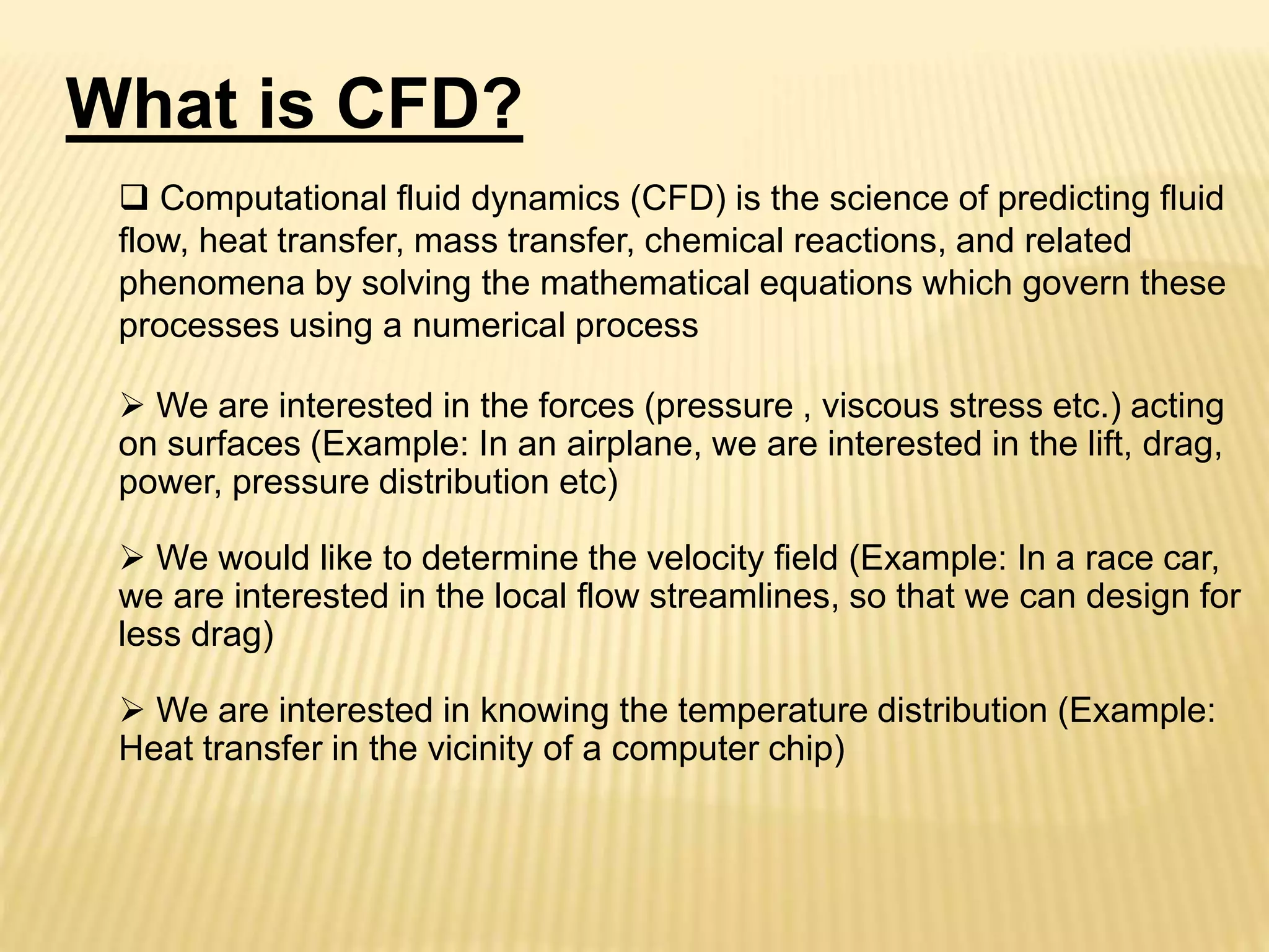
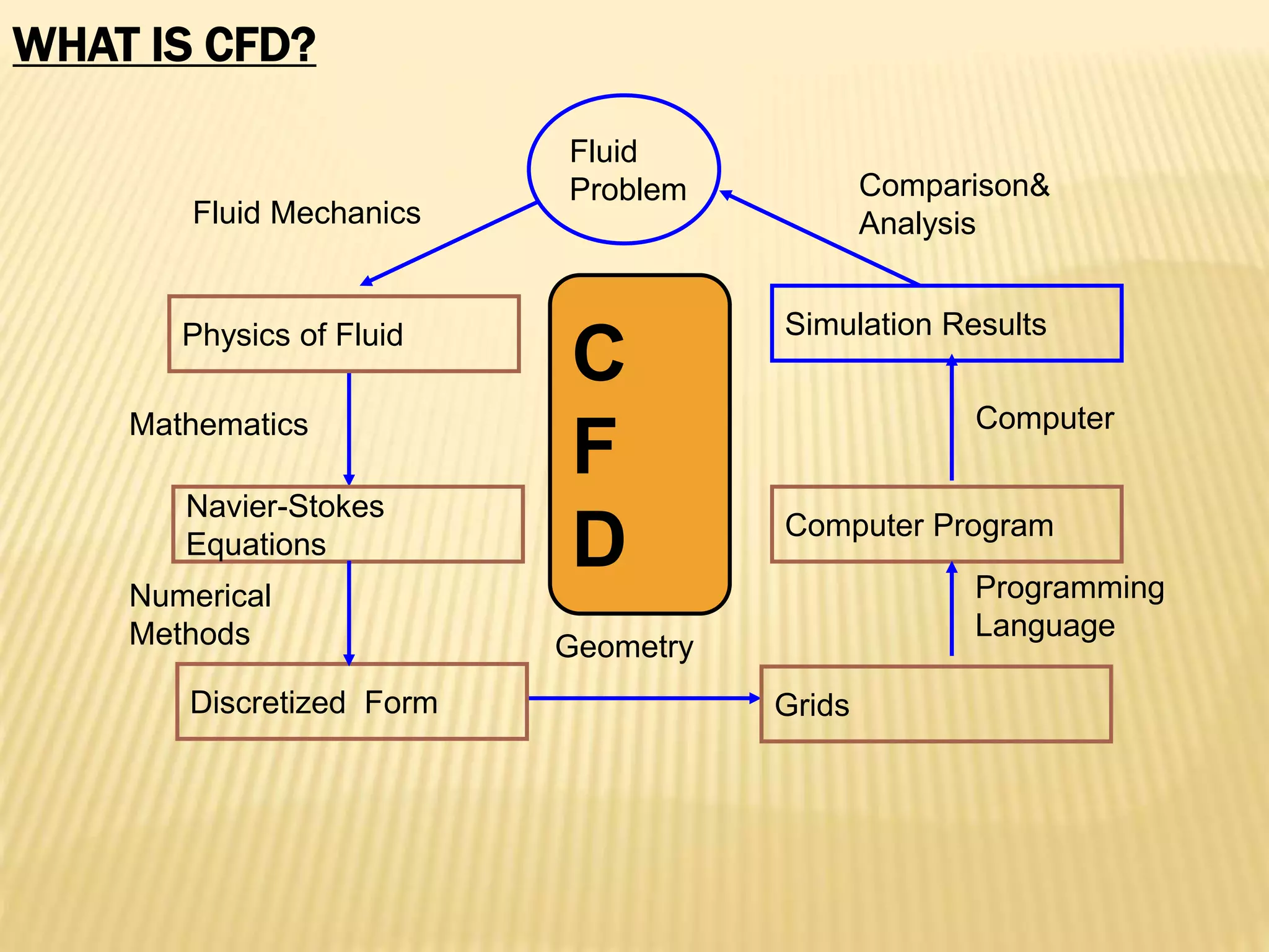
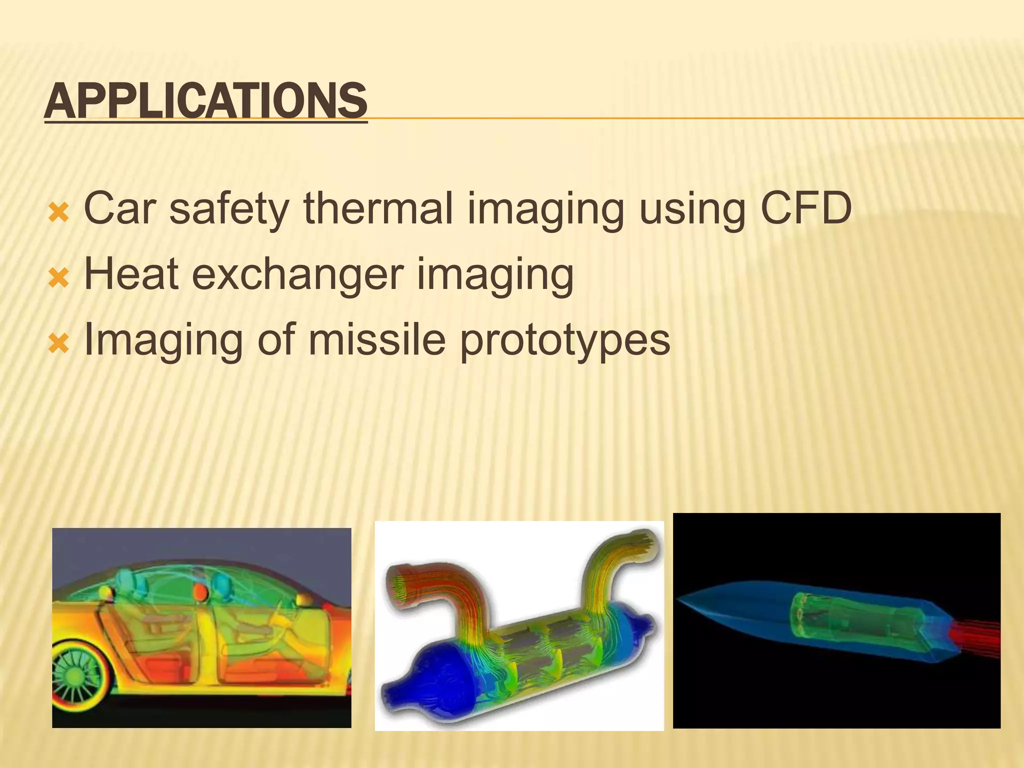
SEMINAR PRESENTATION
ON
FUNDAMENTALS OF COMPUTATIONAL FLUID
DYNAMICS(CFD)
Presented By:-
Pankaj Darbar Koli
B.Tech (Mechanical)
Roll No:-42
Seminar Guide:-
Prof. R.D.Sandhanshiv
R.C.PATEL INSTITUTE OF TECHNOLOGY
(An ISO 9001:2011 Certified Institution & Accredited by NAAC-UGC)
DEPARTMENT OF MECHANICAL ENGINEERING.
 What is Computational Fluid Dynamics(CFD)?
 Why and where use CFD?
 Physics of Fluid
Grids
 Boundary Conditions
 Applications
Advantage
Limitation
 References
CONTENTS
What is CFD?
 Computational fluid dynamics (CFD) is the science of predicting fluid
flow, heat transfer, mass transfer, chemical reactions, and related
phenomena by solving the mathematical equations which govern these
processes using a numerical process
 We are interested in the forces (pressure , viscous stress etc.) acting
on surfaces (Example: In an airplane, we are interested in the lift, drag,
power, pressure distribution etc)
 We would like to determine the velocity field (Example: In a race car,
we are interested in the local flow streamlines, so that we can design for
less drag)
 We are interested in knowing the temperature distribution (Example:
Heat transfer in the vicinity of a computer chip)
WHAT IS CFD?
Mathematics
Navier-Stokes
Equations
Fluid Mechanics
Physics of Fluid
Fluid
Problem
Computer Program
Programming
Language
Simulation Results
Computer
Grids
Geometry
Numerical
Methods
Discretized Form
Comparison&
Analysis
C
F
D
WHY USE CFD?
Simulation(CFD) Experiment
Cost Cheap Expensive
Time Short Long
Scale Any Small/Middle
Information All Measured Points
Repeatable All Some
Security Safe Some Dangerous
WHERE USE CFD?
• Aerospace
• Automotive
• Biomedical
• Chemical
Processing
• HVAC
• Hydraulics
• Power Generation
• Sports
• Marine
Temperature and natural
convection currents in the eye
following laser heating.
Aerospa
ce
Automotive
Biomedicine
WHERE USE CFD?
reactor vessel - prediction of flow
separation and residence time effects.
Streamlines for workstation
ventilation
HVAC
Chemical Processing
Hydraulics
• Aerospace
• Automotive
• Biomedical
• Chemical Processing
• HVAC(Heat
Ventilation Air
Condition)
• Hydraulics
• Power Generation
• Sports
• Marine
WHERE USE CFD?
Flow around cooling towers
Marine
Sports Power Generation
• Aerospace
• Automotive
• Biomedical
• Chemical Processing
• HVAC
• Hydraulics
• Power Generation
• Sports
• Marine
PHYSICS OF FLUID
 Density
ρ
 Fluid = Liquid or Gas
le
compressib
variable
ible
incompress
const





Substance Air(18ºC) Water(20ºC) Honey(20ºC)
Density(kg/m3) 1.275 1000 1446
Viscosity(P) 1.82e-4 1.002e-2 190
Viscosity μ:
resistance to flow of a fluid
)
(
3
Poise
m
Ns









CONSERVATION LAW
in out
M
in
m
 out
m

out
in m
m
dt
dM

 

out
in m
m 
 
0

dt
dM
Mass
Momentum
Energy
DISCRETIZATION
 Discretization Methods
 Finite Difference
Straightforward to apply, simple, sturctured grids
 Finite Element
Any geometries
 Finite Volume
Conservation, any geometries
Analytical Equations Discretized Equations
Discretization
FINITE VOLUME METHOD
General Form of Navier-Stokes Equation
 

 




















q
x
U
x
t i
i
i


 
T
U j ,
,
1



 





S
i
V i
dS
n
dV
x
Integrate over the
Control Volume(CV)
Local change with time Flux Source
 


 




















V
S
i
i
i
V
dV
q
dS
n
x
U
dV
t


Integral Form of Navier-Stokes Equation
Local change
with time in CV
Flux Over
the CV Surface
Source in CV
GRIDS
 Structured Grid
+ all nodes have the same number of elements
around it
– only for simple domains
 Unstructured Grid
+ for all geometries
– irregular data structure
 Block Structured
Grid
BOUNDARY CONDITIONS
 Typical Boundary Conditions
No-slip(Wall), Axisymmetric, Inlet, Outlet, Periodic
Inlet ,u=c,v=0
o
No-slip walls: u=0,v=0
v=0, dp/dr=0,du/dr=0
Outlet, du/dx=0
dv/dy=0,dp/dx=0
r
x
Axisymmetric Periodic boundary
condition in spanwise
direction of an airfoil
APPLICATIONS
 Car safety thermal imaging using CFD
 Heat exchanger imaging
 Imaging of missile prototypes
ADVANTAGES
 Relatively low cost.
 CFD simulations are relatively inexpensive, and costs are
likely to decrease as computers become more powerful.
 Speed.
 CFD simulations can be executed in a short period of
time.
 Ability to simulate real conditions.
 CFD provides the ability to theoretically simulate any
physical condition.
 Comprehensive information.
 CFD allows the analyst to examine a large number of
locations in the region of interest, and yields a
comprehensive set of flow parameters for examination.
LIMITATIONS
• The CFD solutions can only be as accurate as the physical models on
which they are based.
• Solving equations on a computer invariably introduces numerical
errors.
 Round-off error: due to finite word size available on the computer.
Round-off errors will always exist (though they can be small in most
cases).
 Truncation error: due to approximations in the numerical models.
Truncation errors will go to zero as the grid is refined. Mesh refinement
is one way to deal with truncation error.
 Boundary conditions.
 As with physical models, the accuracy of the CFD solution is
only as good as the initial/boundary conditions provided to the
numerical model.
REFERENCES
 www.google.com
 www.wikipedia.com
 www.slideshare.com
THANKS

Fundamentals of Computational Fluid Dynamics

  • 1.
    SEMINAR PRESENTATION ON FUNDAMENTALS OFCOMPUTATIONAL FLUID DYNAMICS(CFD) Presented By:- Pankaj Darbar Koli B.Tech (Mechanical) Roll No:-42 Seminar Guide:- Prof. R.D.Sandhanshiv R.C.PATEL INSTITUTE OF TECHNOLOGY (An ISO 9001:2011 Certified Institution & Accredited by NAAC-UGC) DEPARTMENT OF MECHANICAL ENGINEERING.
  • 2.
     What isComputational Fluid Dynamics(CFD)?  Why and where use CFD?  Physics of Fluid Grids  Boundary Conditions  Applications Advantage Limitation  References CONTENTS
  • 3.
    What is CFD? Computational fluid dynamics (CFD) is the science of predicting fluid flow, heat transfer, mass transfer, chemical reactions, and related phenomena by solving the mathematical equations which govern these processes using a numerical process  We are interested in the forces (pressure , viscous stress etc.) acting on surfaces (Example: In an airplane, we are interested in the lift, drag, power, pressure distribution etc)  We would like to determine the velocity field (Example: In a race car, we are interested in the local flow streamlines, so that we can design for less drag)  We are interested in knowing the temperature distribution (Example: Heat transfer in the vicinity of a computer chip)
  • 4.
    WHAT IS CFD? Mathematics Navier-Stokes Equations FluidMechanics Physics of Fluid Fluid Problem Computer Program Programming Language Simulation Results Computer Grids Geometry Numerical Methods Discretized Form Comparison& Analysis C F D
  • 5.
    WHY USE CFD? Simulation(CFD)Experiment Cost Cheap Expensive Time Short Long Scale Any Small/Middle Information All Measured Points Repeatable All Some Security Safe Some Dangerous
  • 6.
    WHERE USE CFD? •Aerospace • Automotive • Biomedical • Chemical Processing • HVAC • Hydraulics • Power Generation • Sports • Marine Temperature and natural convection currents in the eye following laser heating. Aerospa ce Automotive Biomedicine
  • 7.
    WHERE USE CFD? reactorvessel - prediction of flow separation and residence time effects. Streamlines for workstation ventilation HVAC Chemical Processing Hydraulics • Aerospace • Automotive • Biomedical • Chemical Processing • HVAC(Heat Ventilation Air Condition) • Hydraulics • Power Generation • Sports • Marine
  • 8.
    WHERE USE CFD? Flowaround cooling towers Marine Sports Power Generation • Aerospace • Automotive • Biomedical • Chemical Processing • HVAC • Hydraulics • Power Generation • Sports • Marine
  • 9.
    PHYSICS OF FLUID Density ρ  Fluid = Liquid or Gas le compressib variable ible incompress const      Substance Air(18ºC) Water(20ºC) Honey(20ºC) Density(kg/m3) 1.275 1000 1446 Viscosity(P) 1.82e-4 1.002e-2 190 Viscosity μ: resistance to flow of a fluid ) ( 3 Poise m Ns         
  • 10.
    CONSERVATION LAW in out M in m out m  out in m m dt dM     out in m m    0  dt dM Mass Momentum Energy
  • 11.
    DISCRETIZATION  Discretization Methods Finite Difference Straightforward to apply, simple, sturctured grids  Finite Element Any geometries  Finite Volume Conservation, any geometries Analytical Equations Discretized Equations Discretization
  • 12.
    FINITE VOLUME METHOD GeneralForm of Navier-Stokes Equation                          q x U x t i i i     T U j , , 1           S i V i dS n dV x Integrate over the Control Volume(CV) Local change with time Flux Source                           V S i i i V dV q dS n x U dV t   Integral Form of Navier-Stokes Equation Local change with time in CV Flux Over the CV Surface Source in CV
  • 13.
    GRIDS  Structured Grid +all nodes have the same number of elements around it – only for simple domains  Unstructured Grid + for all geometries – irregular data structure  Block Structured Grid
  • 14.
    BOUNDARY CONDITIONS  TypicalBoundary Conditions No-slip(Wall), Axisymmetric, Inlet, Outlet, Periodic Inlet ,u=c,v=0 o No-slip walls: u=0,v=0 v=0, dp/dr=0,du/dr=0 Outlet, du/dx=0 dv/dy=0,dp/dx=0 r x Axisymmetric Periodic boundary condition in spanwise direction of an airfoil
  • 15.
    APPLICATIONS  Car safetythermal imaging using CFD  Heat exchanger imaging  Imaging of missile prototypes
  • 16.
    ADVANTAGES  Relatively lowcost.  CFD simulations are relatively inexpensive, and costs are likely to decrease as computers become more powerful.  Speed.  CFD simulations can be executed in a short period of time.  Ability to simulate real conditions.  CFD provides the ability to theoretically simulate any physical condition.  Comprehensive information.  CFD allows the analyst to examine a large number of locations in the region of interest, and yields a comprehensive set of flow parameters for examination.
  • 17.
    LIMITATIONS • The CFDsolutions can only be as accurate as the physical models on which they are based. • Solving equations on a computer invariably introduces numerical errors.  Round-off error: due to finite word size available on the computer. Round-off errors will always exist (though they can be small in most cases).  Truncation error: due to approximations in the numerical models. Truncation errors will go to zero as the grid is refined. Mesh refinement is one way to deal with truncation error.  Boundary conditions.  As with physical models, the accuracy of the CFD solution is only as good as the initial/boundary conditions provided to the numerical model.
  • 18.
  • 19.