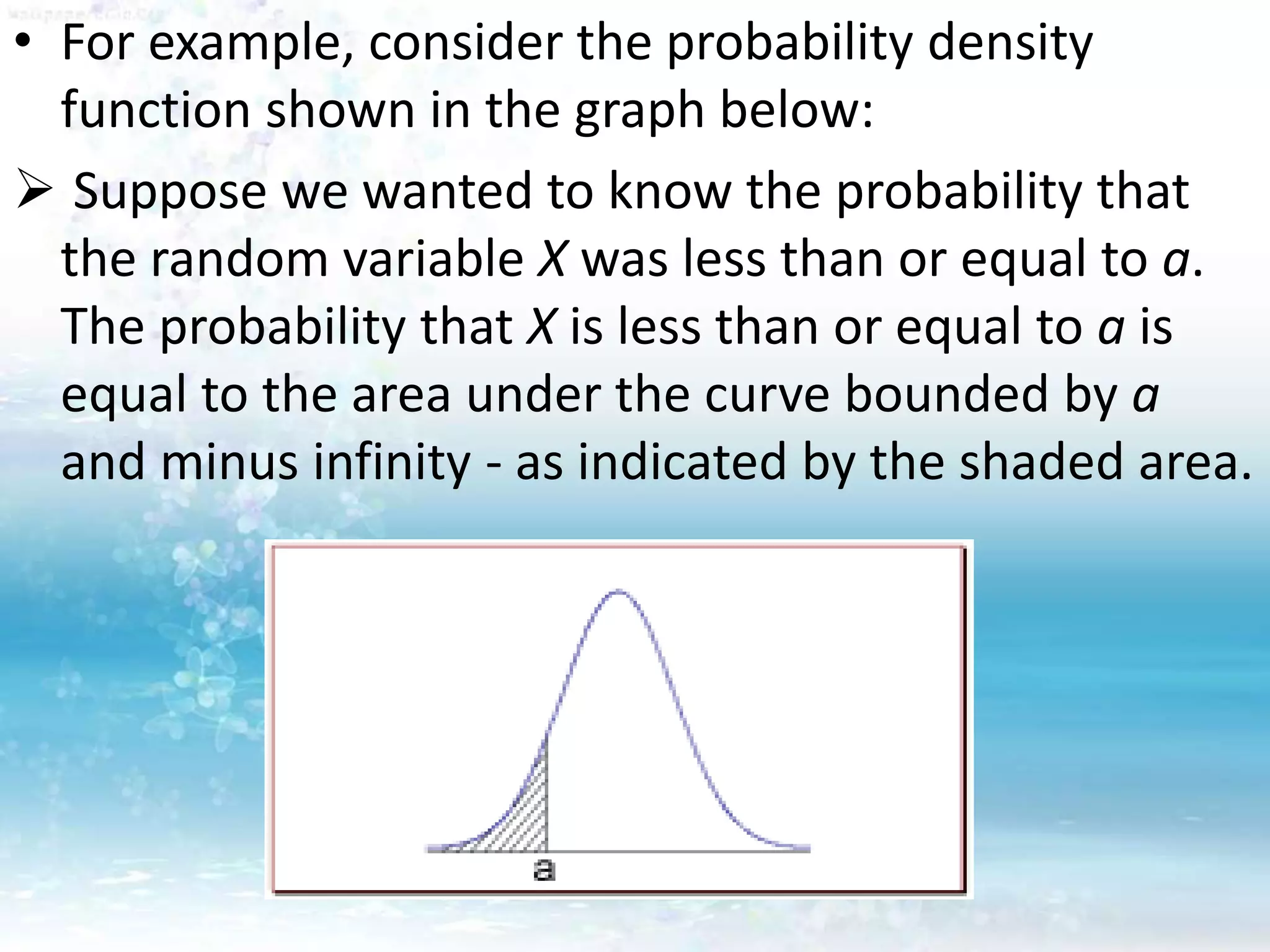
DISCREET AND CONTINUOUS
PROBABILITY
PRESENTED BY:
Noopur Joshi
MSc. I SEM
DEPARTMENT:
BIOTECHNOLOGY
PROBABILITY
AN INTRODUCTION
• Probability is a measure of the expectation that an
event will occur or a statement is true.
• Probabilities are given a value between 0 (will not
occur) and 1 (will occur).
• The higher the probability of an event, the more
certain we are that the event will occur.
• The concept has been given an axiomatic
mathematical derivation in probability theory,
which is used widely in such areas of study as
mathematics, statistics, finance, gambling, science,
artificial intelligence/machine learning and
philosophy to, for example, draw inferences about
the expected frequency of events.
• Probability theory is also used to describe the
underlying mechanics and regularities of complex
systems.
Etymology
• The word Probability derives from the Latin
probabilitas, which can also mean probity, a
measure of the authority of a witness in a legal case
in Europe, and often correlated with the witness's
nobility.
• In a sense, this differs much from the modern
meaning of probability, which, in contrast, is a
measure of the weight of empirical evidence, and is
arrived at from inductive reasoning and statistical
inference.
Interpretations
• When dealing with experiments that are
random and well-defined in a purely
theoretical setting (like tossing a fair coin),
probabilities describe the statistical number of
outcomes considered divided by the number
of all outcomes (tossing a fair coin twice will
yield HH with probability 1/4, because the
four outcomes HH, HT, TH and TT are
possible).
• When it comes to practical application,
however, the word probability does not have a
singular direct definition.
• There are two major categories of probability
interpretations, whose adherents possess
conflicting views about the fundamental
nature of probability:
• Objectivists assign numbers to describe some
objective or physical state of affairs.
• The most popular version of objective probability is
frequentist probability, which claims that the
probability of a random event denotes the relative
frequency of occurrence of an experiment's
outcome, when repeating the experiment.
• This interpretation considers probability to be the
relative frequency "in the long run" of outcomes.
• A modification of this is propensity probability,
which interprets probability as the tendency of
some experiment to yield a certain outcome, even if
it is performed only once.
• Subjectivists assign numbers per subjective
probability, i.e., as a degree of belief.
• The most popular version of subjective probability
is Bayesian probability, which includes expert
knowledge as well as experimental data to produce
probabilities.
• The expert knowledge is represented by some
(subjective) prior probability distribution. The data
is incorporated in a likelihood function.
• The product of the prior and the likelihood,
normalized, results in a posterior probability
distribution that incorporates all the information
known to date.
Probability Distributions:
Discrete vs. Continuous
• All probability distributions can be classified as
discrete probability distributions or as
continuous probability distributions,
depending on whether they define
probabilities associated with discrete variables
or continuous variables
Discrete vs. Continuous Variables
• If a variable can take on any value between
two specified values, it is called a continuous
variable; otherwise, it is called a discrete
variable
• Suppose the fire department mandates that all fire
fighters must weigh between 150 and 250 pounds.
The weight of a fire fighter would be an example of
a continuous variable; since a fire fighter's weight
could take on any value between 150 and 250
pounds.
• Suppose we flip a coin and count the number of
heads. The number of heads could be any integer
value between 0 and plus infinity. However, it could
not be any number between 0 and plus infinity. We
could not, for example, get 2.5 heads. Therefore,
the number of heads must be a discrete variable.
Just like variables,
probability distributions can
be classified as discrete or
continuous.
Discrete Probability Distributions
• DEFINITION:
If a random variable is a discrete variable, its
probability distribution is called a discrete
probability distribution.
EXAMPLE
• Suppose you flip a coin two times. This simple
statistical experiment can have four possible
outcomes: HH, HT, TH, and TT.
• Now, let the random variable X represent the
number of Heads that result from this experiment
• The random variable X can only take on the values
0, 1, or 2, so it is a discrete random variable.
• The probability distribution for this statistical
experiment appears below
• The above table represents a discrete probability
distribution because it relates each value of a discrete
random variable with its probability of occurrence
Number of
heads
Probability
0 0.25
1 0.50
2 0.25
Continuous Probability Distributions
• DEFINITION:
If a random variable is a continuous variable,
its probability distribution is called a
continuous probability distribution.
• A continuous probability distribution differs from a
discrete probability distribution in several ways:
1. The probability that a continuous random variable
will assume a particular value is zero.
2.As a result, a continuous probability distribution
cannot be expressed in tabular form.
3.Instead, an equation or formula is used to describe
a continuous probability distribution.
• Most often, the equation used to describe a
continuous probability distribution is called a
probability density function.
• Sometimes, it is referred to as a density function, a
PDF, or a pdf. For a continuous probability
distribution, the density function has the following
properties:
• Since the continuous random variable is defined
over a continuous range of values (called the
domain of the variable), the graph of the density
function will also be continuous over that range.
• The area bounded by the curve of the density
function and the x-axis is equal to 1, when
computed over the domain of the variable.
• The probability that a random variable assumes a
value between a and b is equal to the area under
the density function bounded by a and b.
• For example, consider the probability density
function shown in the graph below:
 Suppose we wanted to know the probability that
the random variable X was less than or equal to a.
The probability that X is less than or equal to a is
equal to the area under the curve bounded by a
and minus infinity - as indicated by the shaded area.
THE END
• Note: The shaded area in the graph represents
the probability that the random variable X is
less than or equal to a. This is a cumulative
probability. However, the probability that X is
exactly equal to a would be zero. A continuous
random variable can take on an infinite
number of values. The probability that it will
equal a specific value (such as a) is always
zero.

Discreet and continuous probability

  • 1.
    DISCREET AND CONTINUOUS PROBABILITY PRESENTEDBY: Noopur Joshi MSc. I SEM DEPARTMENT: BIOTECHNOLOGY
  • 2.
  • 3.
    • Probability isa measure of the expectation that an event will occur or a statement is true. • Probabilities are given a value between 0 (will not occur) and 1 (will occur). • The higher the probability of an event, the more certain we are that the event will occur.
  • 4.
    • The concepthas been given an axiomatic mathematical derivation in probability theory, which is used widely in such areas of study as mathematics, statistics, finance, gambling, science, artificial intelligence/machine learning and philosophy to, for example, draw inferences about the expected frequency of events. • Probability theory is also used to describe the underlying mechanics and regularities of complex systems.
  • 5.
    Etymology • The wordProbability derives from the Latin probabilitas, which can also mean probity, a measure of the authority of a witness in a legal case in Europe, and often correlated with the witness's nobility. • In a sense, this differs much from the modern meaning of probability, which, in contrast, is a measure of the weight of empirical evidence, and is arrived at from inductive reasoning and statistical inference.
  • 6.
    Interpretations • When dealingwith experiments that are random and well-defined in a purely theoretical setting (like tossing a fair coin), probabilities describe the statistical number of outcomes considered divided by the number of all outcomes (tossing a fair coin twice will yield HH with probability 1/4, because the four outcomes HH, HT, TH and TT are possible).
  • 7.
    • When itcomes to practical application, however, the word probability does not have a singular direct definition. • There are two major categories of probability interpretations, whose adherents possess conflicting views about the fundamental nature of probability:
  • 8.
    • Objectivists assignnumbers to describe some objective or physical state of affairs. • The most popular version of objective probability is frequentist probability, which claims that the probability of a random event denotes the relative frequency of occurrence of an experiment's outcome, when repeating the experiment. • This interpretation considers probability to be the relative frequency "in the long run" of outcomes. • A modification of this is propensity probability, which interprets probability as the tendency of some experiment to yield a certain outcome, even if it is performed only once.
  • 9.
    • Subjectivists assignnumbers per subjective probability, i.e., as a degree of belief. • The most popular version of subjective probability is Bayesian probability, which includes expert knowledge as well as experimental data to produce probabilities. • The expert knowledge is represented by some (subjective) prior probability distribution. The data is incorporated in a likelihood function. • The product of the prior and the likelihood, normalized, results in a posterior probability distribution that incorporates all the information known to date.
  • 10.
    Probability Distributions: Discrete vs.Continuous • All probability distributions can be classified as discrete probability distributions or as continuous probability distributions, depending on whether they define probabilities associated with discrete variables or continuous variables
  • 11.
    Discrete vs. ContinuousVariables • If a variable can take on any value between two specified values, it is called a continuous variable; otherwise, it is called a discrete variable
  • 12.
    • Suppose thefire department mandates that all fire fighters must weigh between 150 and 250 pounds. The weight of a fire fighter would be an example of a continuous variable; since a fire fighter's weight could take on any value between 150 and 250 pounds. • Suppose we flip a coin and count the number of heads. The number of heads could be any integer value between 0 and plus infinity. However, it could not be any number between 0 and plus infinity. We could not, for example, get 2.5 heads. Therefore, the number of heads must be a discrete variable.
  • 13.
    Just like variables, probabilitydistributions can be classified as discrete or continuous.
  • 14.
    Discrete Probability Distributions •DEFINITION: If a random variable is a discrete variable, its probability distribution is called a discrete probability distribution.
  • 15.
    EXAMPLE • Suppose youflip a coin two times. This simple statistical experiment can have four possible outcomes: HH, HT, TH, and TT. • Now, let the random variable X represent the number of Heads that result from this experiment • The random variable X can only take on the values 0, 1, or 2, so it is a discrete random variable.
  • 16.
    • The probabilitydistribution for this statistical experiment appears below • The above table represents a discrete probability distribution because it relates each value of a discrete random variable with its probability of occurrence Number of heads Probability 0 0.25 1 0.50 2 0.25
  • 17.
    Continuous Probability Distributions •DEFINITION: If a random variable is a continuous variable, its probability distribution is called a continuous probability distribution.
  • 18.
    • A continuousprobability distribution differs from a discrete probability distribution in several ways: 1. The probability that a continuous random variable will assume a particular value is zero. 2.As a result, a continuous probability distribution cannot be expressed in tabular form. 3.Instead, an equation or formula is used to describe a continuous probability distribution.
  • 19.
    • Most often,the equation used to describe a continuous probability distribution is called a probability density function. • Sometimes, it is referred to as a density function, a PDF, or a pdf. For a continuous probability distribution, the density function has the following properties:
  • 20.
    • Since thecontinuous random variable is defined over a continuous range of values (called the domain of the variable), the graph of the density function will also be continuous over that range. • The area bounded by the curve of the density function and the x-axis is equal to 1, when computed over the domain of the variable. • The probability that a random variable assumes a value between a and b is equal to the area under the density function bounded by a and b.
  • 21.
    • For example,consider the probability density function shown in the graph below:  Suppose we wanted to know the probability that the random variable X was less than or equal to a. The probability that X is less than or equal to a is equal to the area under the curve bounded by a and minus infinity - as indicated by the shaded area.
  • 22.
  • 23.
    • Note: Theshaded area in the graph represents the probability that the random variable X is less than or equal to a. This is a cumulative probability. However, the probability that X is exactly equal to a would be zero. A continuous random variable can take on an infinite number of values. The probability that it will equal a specific value (such as a) is always zero.