Chapter-6-Random Variables & Probability distributions-3.doc

L
Le
ec
ct
tu
ur
re
e n
no
ot
te
es
s o
on
n I
In
nt
tr
ro
od
du
uc
ct
ti
io
on
n t
to
o S
St
ta
at
ti
is
st
ti
ic
cs
s (
(S
St
ta
at
t 1
17
73
3)
) C
Ch
ha
ap
pt
te
er
r 6
6:
: R
Ra
an
nd
do
om
m V
Va
ar
ri
ia
ab
bl
le
es
s &
& P
Pr
ro
ob
b.
.
d
di
is
st
tr
ri
ib
bu
ut
ti
io
on
ns
s
Page 1 of 18
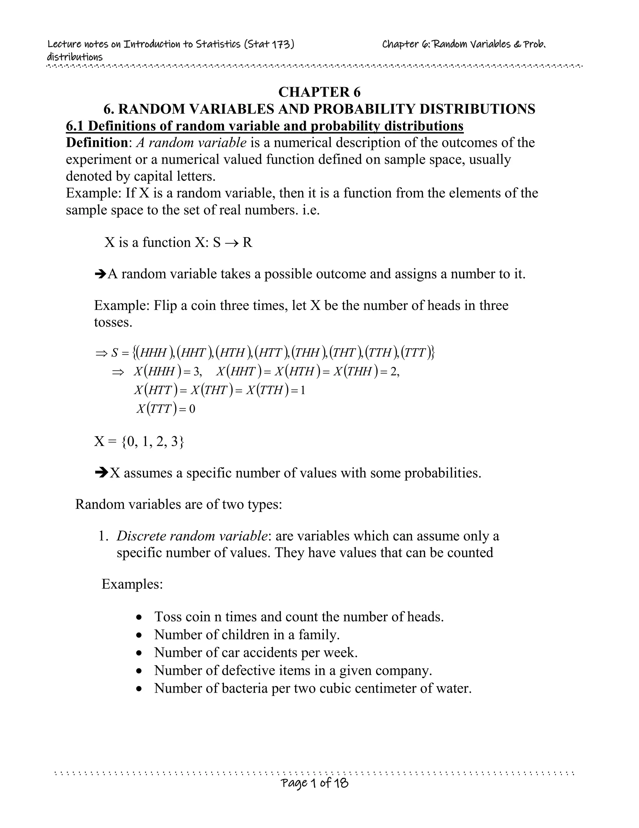
CHAPTER 6
6. RANDOM VARIABLES AND PROBABILITY DISTRIBUTIONS
6.1 Definitions of random variable and probability distributions
Definition: A random variable is a numerical description of the outcomes of the
experiment or a numerical valued function defined on sample space, usually
denoted by capital letters.
Example: If X is a random variable, then it is a function from the elements of the
sample space to the set of real numbers. i.e.
X is a function X: S  R
A random variable takes a possible outcome and assigns a number to it.
Example: Flip a coin three times, let X be the number of heads in three
tosses.
               
 
       
     
  0
1
,
2
,
3
,
,
,
,
,
,
,











TTT
X
TTH
X
THT
X
HTT
X
THH
X
HTH
X
HHT
X
HHH
X
TTT
TTH
THT
THH
HTT
HTH
HHT
HHH
S
X = {0, 1, 2, 3}
X assumes a specific number of values with some probabilities.
Random variables are of two types:
1. Discrete random variable: are variables which can assume only a
specific number of values. They have values that can be counted
Examples:
 Toss coin n times and count the number of heads.
 Number of children in a family.
 Number of car accidents per week.
 Number of defective items in a given company.
 Number of bacteria per two cubic centimeter of water.

L
Le
ec
ct
tu
ur
re
e n
no
ot
te
es
s o
on
n I
In
nt
tr
ro
od
du
uc
ct
ti
io
on
n t
to
o S
St
ta
at
ti
is
st
ti
ic
cs
s (
(S
St
ta
at
t 1
17
73
3)
) C
Ch
ha
ap
pt
te
er
r 6
6:
: R
Ra
an
nd
do
om
m V
Va
ar
ri
ia
ab
bl
le
es
s &
& P
Pr
ro
ob
b.
.
d
di
is
st
tr
ri
ib
bu
ut
ti
io
on
ns
s
Page 2 of 18
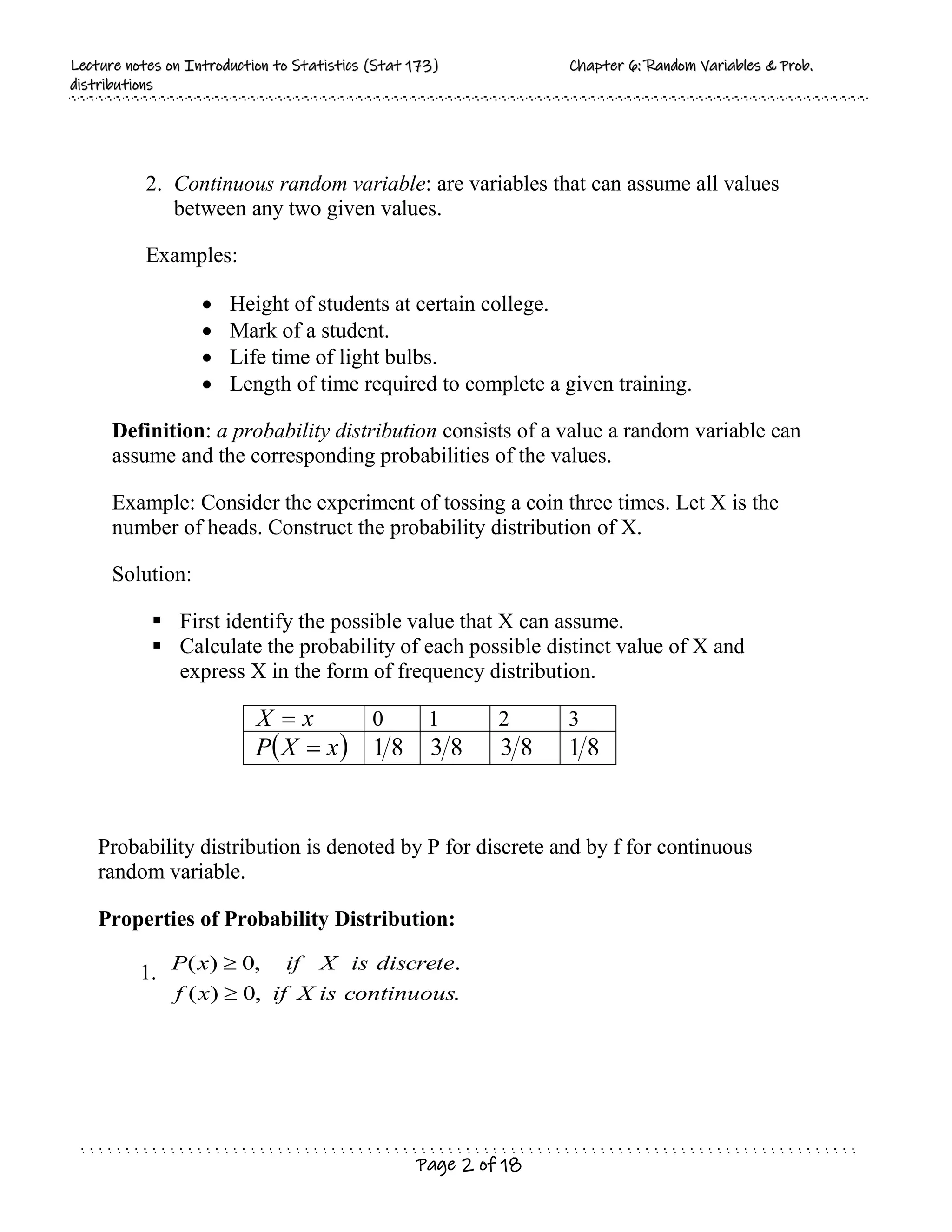
2. Continuous random variable: are variables that can assume all values
between any two given values.
Examples:
 Height of students at certain college.
 Mark of a student.
 Life time of light bulbs.
 Length of time required to complete a given training.
Definition: a probability distribution consists of a value a random variable can
assume and the corresponding probabilities of the values.
Example: Consider the experiment of tossing a coin three times. Let X is the
number of heads. Construct the probability distribution of X.
Solution:
 First identify the possible value that X can assume.
 Calculate the probability of each possible distinct value of X and
express X in the form of frequency distribution.
x
X  0 1 2 3
 
x
X
P  8
1 8
3 8
3 8
1
Probability distribution is denoted by P for discrete and by f for continuous
random variable.
Properties of Probability Distribution:
1.
.
,
0
)
(
.
,
0
)
(
continuous
is
X
if
x
f
discrete
is
X
if
x
P



L
Le
ec
ct
tu
ur
re
e n
no
ot
te
es
s o
on
n I
In
nt
tr
ro
od
du
uc
ct
ti
io
on
n t
to
o S
St
ta
at
ti
is
st
ti
ic
cs
s (
(S
St
ta
at
t 1
17
73
3)
) C
Ch
ha
ap
pt
te
er
r 6
6:
: R
Ra
an
nd
do
om
m V
Va
ar
ri
ia
ab
bl
le
es
s &
& P
Pr
ro
ob
b.
.
d
di
is
st
tr
ri
ib
bu
ut
ti
io
on
ns
s
Page 3 of 18
2.
 
.
,
1
)
(
.
,
1
continuous
is
if
dx
x
f
discrete
is
X
if
x
X
P
x
x





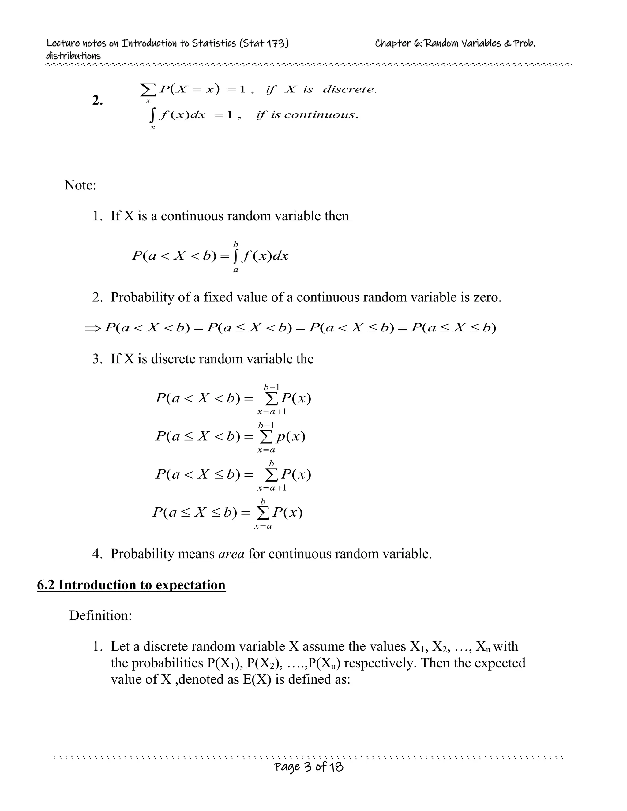
Note:
1. If X is a continuous random variable then




b
a
dx
x
f
b
X
a
P )
(
)
(
2. Probability of a fixed value of a continuous random variable is zero.
)
(
)
(
)
(
)
( b
X
a
P
b
X
a
P
b
X
a
P
b
X
a
P 











3. If X is discrete random variable the
























b
a
x
b
a
x
b
a
x
b
a
x
x
P
b
X
a
P
x
P
b
X
a
P
x
p
b
X
a
P
x
P
b
X
a
P
)
(
)
(
)
(
)
(
)
(
)
(
)
(
)
(
1
1
1
1
4. Probability means area for continuous random variable.
6.2 Introduction to expectation
Definition:
1. Let a discrete random variable X assume the values X1, X2, …, Xn with
the probabilities P(X1), P(X2), ….,P(Xn) respectively. Then the expected
value of X ,denoted as E(X) is defined as:

L
Le
ec
ct
tu
ur
re
e n
no
ot
te
es
s o
on
n I
In
nt
tr
ro
od
du
uc
ct
ti
io
on
n t
to
o S
St
ta
at
ti
is
st
ti
ic
cs
s (
(S
St
ta
at
t 1
17
73
3)
) C
Ch
ha
ap
pt
te
er
r 6
6:
: R
Ra
an
nd
do
om
m V
Va
ar
ri
ia
ab
bl
le
es
s &
& P
Pr
ro
ob
b.
.
d
di
is
st
tr
ri
ib
bu
ut
ti
io
on
ns
s
Page 4 of 18







n
i
i
i
n
n
X
P
X
X
P
X
X
P
X
X
P
X
X
E
1
2
2
1
1
)
(
)
(
....
)
(
)
(
)
(
2. Let X be a continuous random variable assuming the values in the
interval (a, b) such that 1
)
( 

b
a
dx
x
f ,then


b
a
dx
x
f
x
X
E )
(
)
(
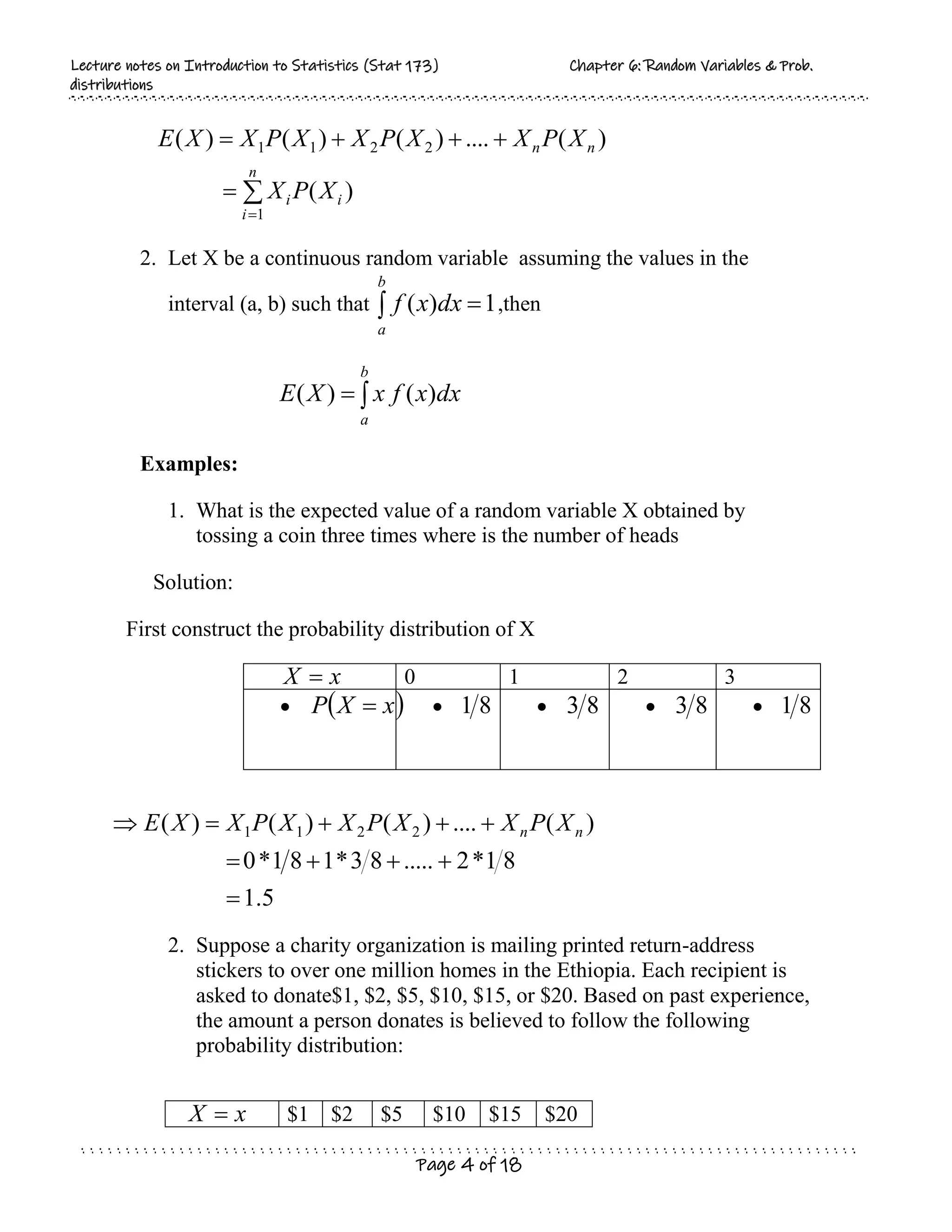
Examples:
1. What is the expected value of a random variable X obtained by
tossing a coin three times where is the number of heads
Solution:
First construct the probability distribution of X
x
X  0 1 2 3
  
x
X
P   8
1  8
3  8
3  8
1
2. Suppose a charity organization is mailing printed return-address
stickers to over one million homes in the Ethiopia. Each recipient is
asked to donate$1, $2, $5, $10, $15, or $20. Based on past experience,
the amount a person donates is believed to follow the following
probability distribution:
x
X  $1 $2 $5 $10 $15 $20
5
.
1
8
1
*
2
.....
8
3
*
1
8
1
*
0
)
(
....
)
(
)
(
)
( 2
2
1
1









 n
n X
P
X
X
P
X
X
P
X
X
E

L
Le
ec
ct
tu
ur
re
e n
no
ot
te
es
s o
on
n I
In
nt
tr
ro
od
du
uc
ct
ti
io
on
n t
to
o S
St
ta
at
ti
is
st
ti
ic
cs
s (
(S
St
ta
at
t 1
17
73
3)
) C
Ch
ha
ap
pt
te
er
r 6
6:
: R
Ra
an
nd
do
om
m V
Va
ar
ri
ia
ab
bl
le
es
s &
& P
Pr
ro
ob
b.
.
d
di
is
st
tr
ri
ib
bu
ut
ti
io
on
ns
s
Page 5 of 18
What is expected that an average donor to contribute?
Solution:
x
X  $1 $2 $5 $10 $15 $20 Total
 
x
X
P  0.1 0.2 0.3 0.2 0.15 0.05 1
)
( x
X
xP  0.1 0.4 1.5 2 2.25 1 7.25
25
.
7
$
)
(
)
(
6
1



 

i
i
i x
X
P
x
X
E
Mean and Variance of a random variable
Let X is given random variable.
1. The expected value of X is its mean )
(X
E
X
of
Mean 

2. The variance of X is given by:
2
2
)]
(
[
)
(
)
var( X
E
X
E
X
X
of
Variance 


Where:
ar
Examples:
1. Find the mean and the variance of a random variable X in example 2
above.
Solutions:
x
X  $1 $2 $5 $10 $15 $20 Total
 
x
X
P  0.1 0.2 0.3 0.2 0.15 0.05 1
)
( x
X
xP  0.1 0.4 1.5 2 2.25 1 7.25
 
x
X
P  0.1 0.2 0.3 0.2 0.15 0.05

L
Le
ec
ct
tu
ur
re
e n
no
ot
te
es
s o
on
n I
In
nt
tr
ro
od
du
uc
ct
ti
io
on
n t
to
o S
St
ta
at
ti
is
st
ti
ic
cs
s (
(S
St
ta
at
t 1
17
73
3)
) C
Ch
ha
ap
pt
te
er
r 6
6:
: R
Ra
an
nd
do
om
m V
Va
ar
ri
ia
ab
bl
le
es
s &
& P
Pr
ro
ob
b.
.
d
di
is
st
tr
ri
ib
bu
ut
ti
io
on
ns
s
Page 6 of 18
)
(
2
x
X
P
x  0.1 0.8 7.5 20 33.75 20 82.15
2. Two dice are rolled. Let X is a random variable denoting the sum of the
numbers on the two dice.
i) Give the probability distribution of X
ii) Compute the expected value of X and its variance
There are some general rules for mathematical expectation.
Let X and Y are random variables and k is a constant.
RULE 1 k
k
E 
)
(
RULE 2 0
)
( 
k
Var
RULE 3 )
(
)
( X
kE
kX
E 
RULE 4 )
(
)
( 2
X
Var
k
kX
Var 
RULE 5 )
(
)
(
)
( Y
E
X
E
Y
X
E 


6.3 Common Discrete Probability Distributions
1. Binomial Distribution
A binomial experiment is a probability experiment that satisfies the following
four requirements called assumptions of a binomial distribution.
1. The experiment consists of n identical trials.
2. Each trial has only one of the two possible mutually exclusive
outcomes, success or a failure.
3. The probability of each outcome does not change from trial to trial, and
4. The trials are independent, thus we must sample with replacement.
59
.
29
25
.
7
15
.
82
)]
(
[
)
(
)
(
25
.
7
)
(
2
2
2







X
E
X
E
X
Var
X
E

L
Le
ec
ct
tu
ur
re
e n
no
ot
te
es
s o
on
n I
In
nt
tr
ro
od
du
uc
ct
ti
io
on
n t
to
o S
St
ta
at
ti
is
st
ti
ic
cs
s (
(S
St
ta
at
t 1
17
73
3)
) C
Ch
ha
ap
pt
te
er
r 6
6:
: R
Ra
an
nd
do
om
m V
Va
ar
ri
ia
ab
bl
le
es
s &
& P
Pr
ro
ob
b.
.
d
di
is
st
tr
ri
ib
bu
ut
ti
io
on
ns
s
Page 7 of 18
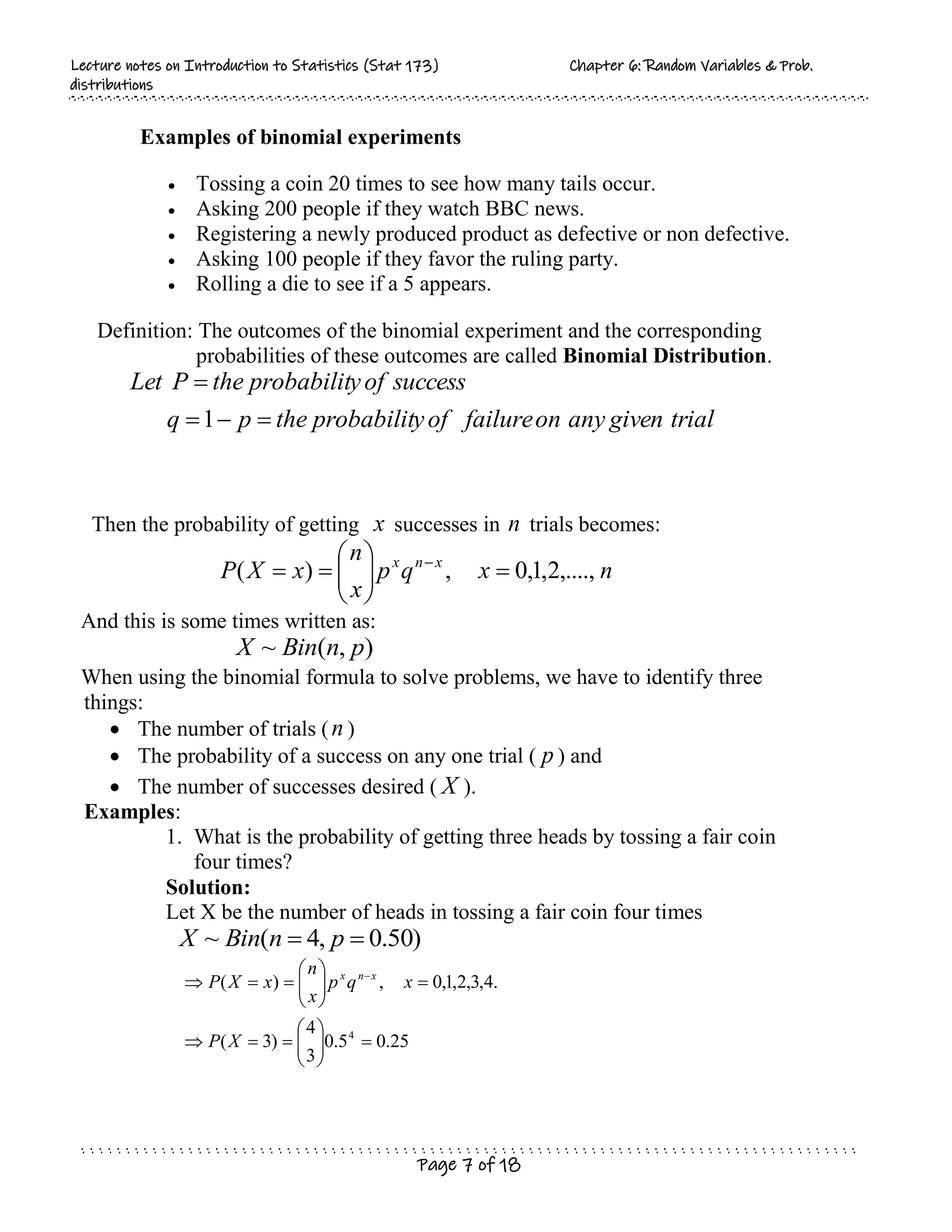
Examples of binomial experiments
 Tossing a coin 20 times to see how many tails occur.
 Asking 200 people if they watch BBC news.
 Registering a newly produced product as defective or non defective.
 Asking 100 people if they favor the ruling party.
 Rolling a die to see if a 5 appears.
Definition: The outcomes of the binomial experiment and the corresponding
probabilities of these outcomes are called Binomial Distribution.
trial
given
any
on
failure
of
y
probabilit
the
p
q
success
of
y
probabilit
the
P
Let




1
Then the probability of getting x successes in n trials becomes:
n
x
q
p
x
n
x
X
P x
n
x
,....,
2
,
1
,
0
,
)
( 









 
And this is some times written as:
)
,
(
~ p
n
Bin
X
When using the binomial formula to solve problems, we have to identify three
things:
 The number of trials (n )
 The probability of a success on any one trial ( p ) and
 The number of successes desired ( X ).
Examples:
1. What is the probability of getting three heads by tossing a fair coin
four times?
Solution:
Let X be the number of heads in tossing a fair coin four times
)
50
.
0
,
4
(
~ 
 p
n
Bin
X
25
.
0
5
.
0
3
4
)
3
(
.
4
,
3
,
2
,
1
,
0
,
)
(
4























 
X
P
x
q
p
x
n
x
X
P x
n
x

L
Le
ec
ct
tu
ur
re
e n
no
ot
te
es
s o
on
n I
In
nt
tr
ro
od
du
uc
ct
ti
io
on
n t
to
o S
St
ta
at
ti
is
st
ti
ic
cs
s (
(S
St
ta
at
t 1
17
73
3)
) C
Ch
ha
ap
pt
te
er
r 6
6:
: R
Ra
an
nd
do
om
m V
Va
ar
ri
ia
ab
bl
le
es
s &
& P
Pr
ro
ob
b.
.
d
di
is
st
tr
ri
ib
bu
ut
ti
io
on
ns
s
Page 8 of 18
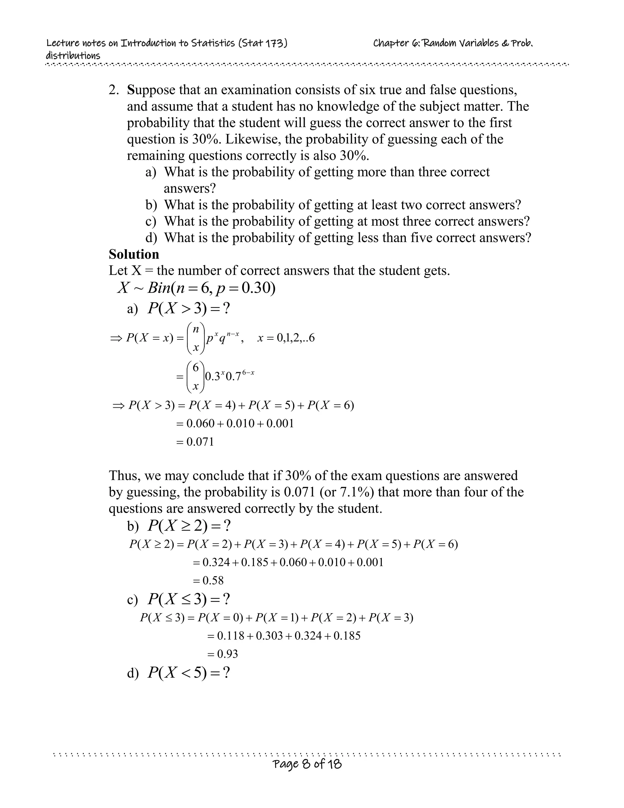
2. Suppose that an examination consists of six true and false questions,
and assume that a student has no knowledge of the subject matter. The
probability that the student will guess the correct answer to the first
question is 30%. Likewise, the probability of guessing each of the
remaining questions correctly is also 30%.
a) What is the probability of getting more than three correct
answers?
b) What is the probability of getting at least two correct answers?
c) What is the probability of getting at most three correct answers?
d) What is the probability of getting less than five correct answers?
Solution
Let X = the number of correct answers that the student gets.
)
30
.
0
,
6
(
~ 
 p
n
Bin
X
a) ?
)
3
( 

X
P
Thus, we may conclude that if 30% of the exam questions are answered
by guessing, the probability is 0.071 (or 7.1%) that more than four of the
questions are answered correctly by the student.
b) ?
)
2
( 

X
P
58
.
0
001
.
0
010
.
0
060
.
0
185
.
0
324
.
0
)
6
(
)
5
(
)
4
(
)
3
(
)
2
(
)
2
(
















 X
P
X
P
X
P
X
P
X
P
X
P
c) ?
)
3
( 

X
P
93
.
0
185
.
0
324
.
0
303
.
0
118
.
0
)
3
(
)
2
(
)
1
(
)
0
(
)
3
(













 X
P
X
P
X
P
X
P
X
P
d) ?
)
5
( 

X
P
071
.
0
001
.
0
010
.
0
060
.
0
)
6
(
)
5
(
)
4
(
)
3
(
7
.
0
3
.
0
6
6
,..
2
,
1
,
0
,
)
(
6



































X
P
X
P
X
P
X
P
x
x
q
p
x
n
x
X
P
x
x
x
n
x

L
Le
ec
ct
tu
ur
re
e n
no
ot
te
es
s o
on
n I
In
nt
tr
ro
od
du
uc
ct
ti
io
on
n t
to
o S
St
ta
at
ti
is
st
ti
ic
cs
s (
(S
St
ta
at
t 1
17
73
3)
) C
Ch
ha
ap
pt
te
er
r 6
6:
: R
Ra
an
nd
do
om
m V
Va
ar
ri
ia
ab
bl
le
es
s &
& P
Pr
ro
ob
b.
.
d
di
is
st
tr
ri
ib
bu
ut
ti
io
on
ns
s
Page 9 of 18
989
.
0
)
001
.
0
010
.
0
(
1
)}
6
(
)
5
(
{
1
)
5
(
1
)
5
(













X
P
X
P
X
P
X
P
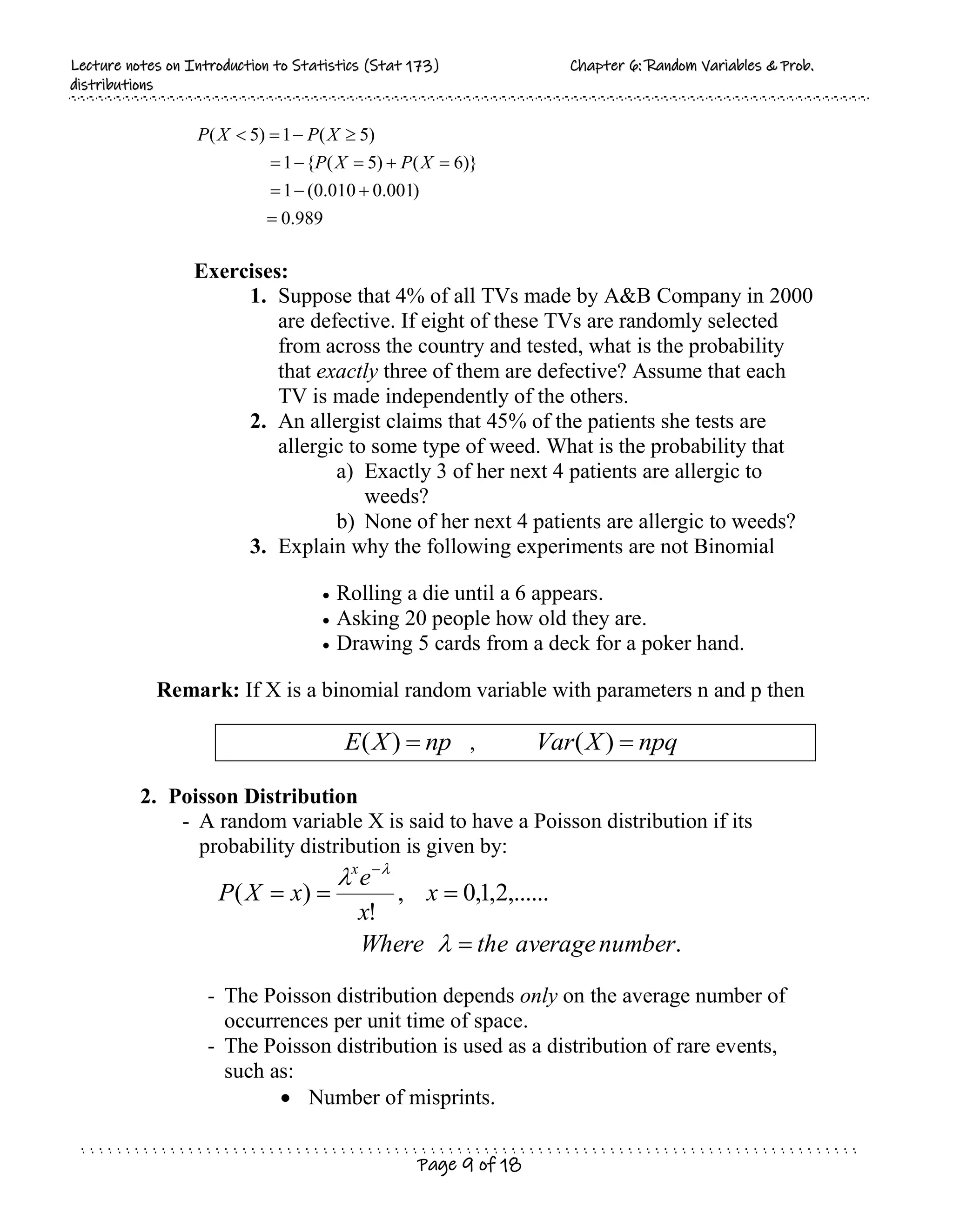
Exercises:
1. Suppose that 4% of all TVs made by A&B Company in 2000
are defective. If eight of these TVs are randomly selected
from across the country and tested, what is the probability
that exactly three of them are defective? Assume that each
TV is made independently of the others.
2. An allergist claims that 45% of the patients she tests are
allergic to some type of weed. What is the probability that
a) Exactly 3 of her next 4 patients are allergic to
weeds?
b) None of her next 4 patients are allergic to weeds?
3. Explain why the following experiments are not Binomial
 Rolling a die until a 6 appears.
 Asking 20 people how old they are.
 Drawing 5 cards from a deck for a poker hand.
Remark: If X is a binomial random variable with parameters n and p then
np
X
E 
)
( , npq
X
Var 
)
(
2. Poisson Distribution
- A random variable X is said to have a Poisson distribution if its
probability distribution is given by:
.
,......
2
,
1
,
0
,
!
)
(
number
average
the
Where
x
x
e
x
X
P
x






 
- The Poisson distribution depends only on the average number of
occurrences per unit time of space.
- The Poisson distribution is used as a distribution of rare events,
such as:
 Number of misprints.

L
Le
ec
ct
tu
ur
re
e n
no
ot
te
es
s o
on
n I
In
nt
tr
ro
od
du
uc
ct
ti
io
on
n t
to
o S
St
ta
at
ti
is
st
ti
ic
cs
s (
(S
St
ta
at
t 1
17
73
3)
) C
Ch
ha
ap
pt
te
er
r 6
6:
: R
Ra
an
nd
do
om
m V
Va
ar
ri
ia
ab
bl
le
es
s &
& P
Pr
ro
ob
b.
.
d
di
is
st
tr
ri
ib
bu
ut
ti
io
on
ns
s
Page 10 of 18
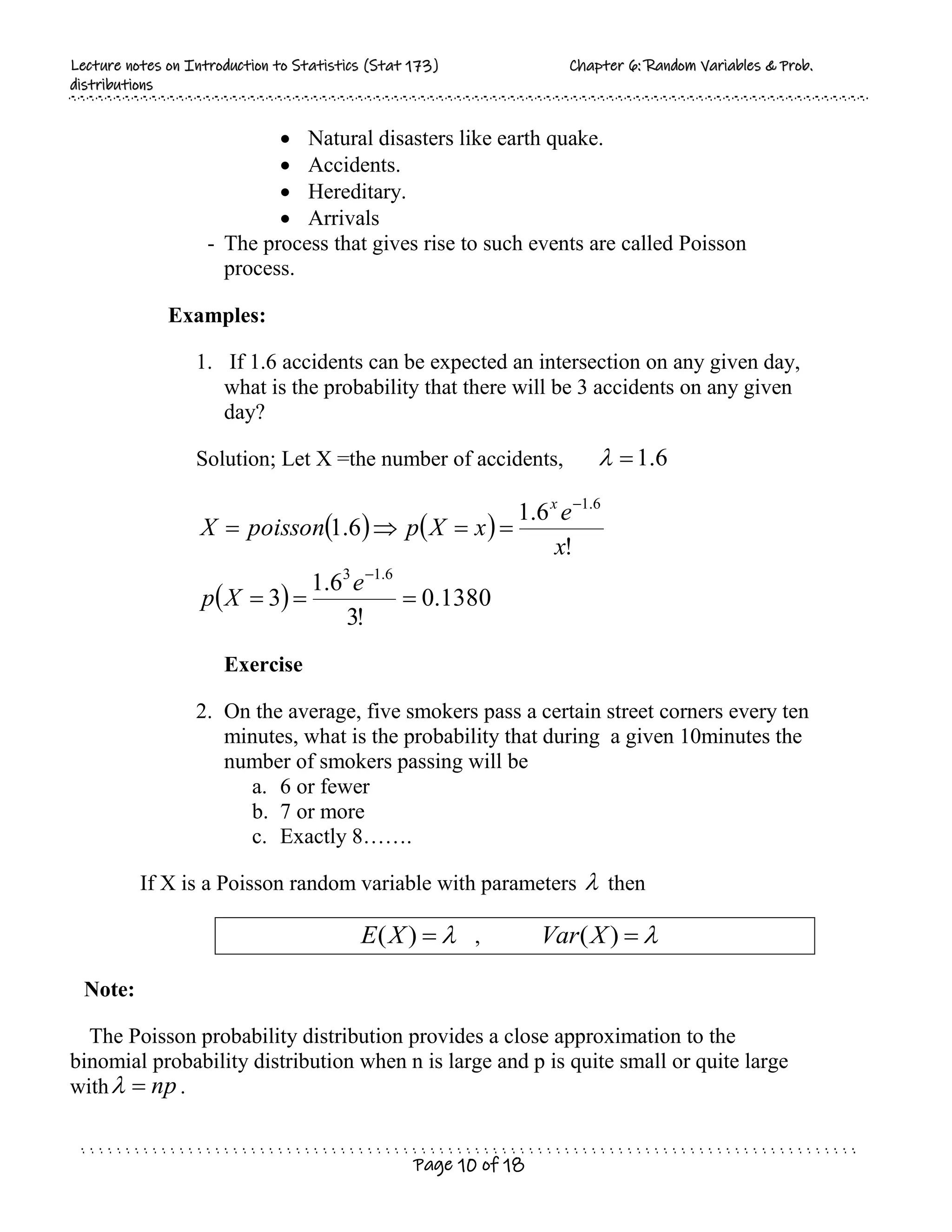
 Natural disasters like earth quake.
 Accidents.
 Hereditary.
 Arrivals
- The process that gives rise to such events are called Poisson
process.
Examples:
1. If 1.6 accidents can be expected an intersection on any given day,
what is the probability that there will be 3 accidents on any given
day?
Solution; Let X =the number of accidents, 6
.
1


   
  1380
.
0
!
3
6
.
1
3
!
6
.
1
6
.
1
6
.
1
3
6
.
1









e
X
p
x
e
x
X
p
poisson
X
x
Exercise
2. On the average, five smokers pass a certain street corners every ten
minutes, what is the probability that during a given 10minutes the
number of smokers passing will be
a. 6 or fewer
b. 7 or more
c. Exactly 8…….
If X is a Poisson random variable with parameters  then


)
(X
E , 

)
(X
Var
Note:
The Poisson probability distribution provides a close approximation to the
binomial probability distribution when n is large and p is quite small or quite large
with np

 .

L
Le
ec
ct
tu
ur
re
e n
no
ot
te
es
s o
on
n I
In
nt
tr
ro
od
du
uc
ct
ti
io
on
n t
to
o S
St
ta
at
ti
is
st
ti
ic
cs
s (
(S
St
ta
at
t 1
17
73
3)
) C
Ch
ha
ap
pt
te
er
r 6
6:
: R
Ra
an
nd
do
om
m V
Va
ar
ri
ia
ab
bl
le
es
s &
& P
Pr
ro
ob
b.
.
d
di
is
st
tr
ri
ib
bu
ut
ti
io
on
ns
s
Page 11 of 18
.
,......
2
,
1
,
0
,
!
)
(
)
(
)
(
number
average
the
np
Where
x
x
e
np
x
X
P
np
x







Usually we use this approximation if 5

np . In other words, if 20

n and
5

np [or 5
)
1
( 
 p
n ], then we may use Poisson distribution as an approximation
to binomial distribution.
Example:
1. Find the binomial probability P(X=3) by using the Poisson distribution
if 01
.
0

p and 200

n
Solution:
1814
.
0
)
99
.
0
(
)
01
.
0
(
3
200
)
3
(
01
.
0
,
200
,
sin
1804
.
0
!
3
2
)
3
(
2
200
*
01
.
0
,
sin
99
3
2
3






















X
P
p
n
Binomial
g
U
e
X
P
np
Poisson
g
U 
6.4 Common Continuous Probability Distributions
1. Normal Distribution
A random variable X is said to have a normal distribution if its probability
density function is given by
.
)
(
),
(
0
,
,
,
2
1
)
(
2
2
2
2
1
on
Distributi
Normal
the
of
Parameters
the
are
and
X
Var
X
E
Where
x
e
x
f
x





























 


L
Le
ec
ct
tu
ur
re
e n
no
ot
te
es
s o
on
n I
In
nt
tr
ro
od
du
uc
ct
ti
io
on
n t
to
o S
St
ta
at
ti
is
st
ti
ic
cs
s (
(S
St
ta
at
t 1
17
73
3)
) C
Ch
ha
ap
pt
te
er
r 6
6:
: R
Ra
an
nd
do
om
m V
Va
ar
ri
ia
ab
bl
le
es
s &
& P
Pr
ro
ob
b.
.
d
di
is
st
tr
ri
ib
bu
ut
ti
io
on
ns
s
Page 12 of 18
Properties of Normal Distribution:
1. It is bell shaped and is symmetrical about its mean and it is mesokurtic.
The maximum ordinate is at 

x and is given by

 2
1
)
( 
x
f
2. It is asymptotic to the axis, i.e., it extends indefinitely in either direction
from the mean.
3. It is a continuous distribution.
4. It is a family of curves, i.e., every unique pair of mean and standard
deviation defines a different normal distribution. Thus, the normal
distribution is completely described by two parameters: mean and
standard deviation.
5. Total area under the curve sums to 1, i.e., the area of the distribution on
each side of the mean is 0.5. 1
)
( 




dx
x
f
6. It is unimodal, i.e., values mound up only in the center of the curve.
7. 


 e
Median
Mean mod
8. The probability that a random variable will have a value between any two
points is equal to the area under the curve between those points.
Note: To facilitate the use of normal distribution, the following distribution known
as the standard normal distribution was derived by using the transformation




X
Z
2
2
1
2
1
)
(
z
e
z
f




Properties of the Standard Normal Distribution:
- Same as a normal distribution, but also...
 Mean is zero
 Variance is one
 Standard Deviation is one
- Areas under the standard normal distribution curve have been tabulated in
various ways. The most common ones are the areas between
.
0 Z
of
value
positive
a
and
Z 

L
Le
ec
ct
tu
ur
re
e n
no
ot
te
es
s o
on
n I
In
nt
tr
ro
od
du
uc
ct
ti
io
on
n t
to
o S
St
ta
at
ti
is
st
ti
ic
cs
s (
(S
St
ta
at
t 1
17
73
3)
) C
Ch
ha
ap
pt
te
er
r 6
6:
: R
Ra
an
nd
do
om
m V
Va
ar
ri
ia
ab
bl
le
es
s &
& P
Pr
ro
ob
b.
.
d
di
is
st
tr
ri
ib
bu
ut
ti
io
on
ns
s
Page 13 of 18
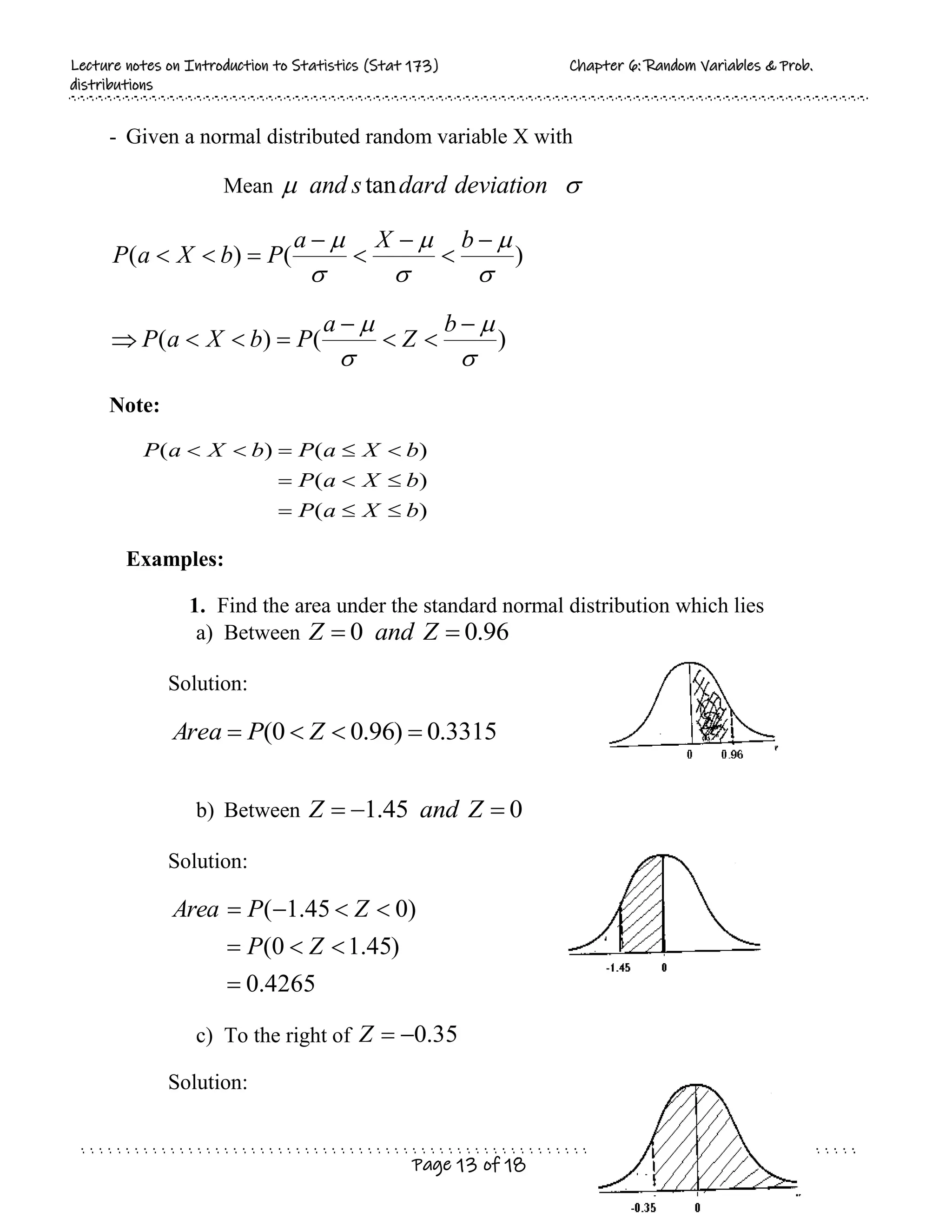
- Given a normal distributed random variable X with
Mean 
 deviation
dard
s
and tan
)
(
)
(





 







b
X
a
P
b
X
a
P
 )
(
)
(



 






b
Z
a
P
b
X
a
P
Note:
)
(
)
(
)
(
)
(
b
X
a
P
b
X
a
P
b
X
a
P
b
X
a
P











Examples:
1. Find the area under the standard normal distribution which lies
a) Between 96
.
0
0 
 Z
and
Z
Solution:
3315
.
0
)
96
.
0
0
( 


 Z
P
Area
b) Between 0
45
.
1 

 Z
and
Z
Solution:
4265
.
0
)
45
.
1
0
(
)
0
45
.
1
(








Z
P
Z
P
Area
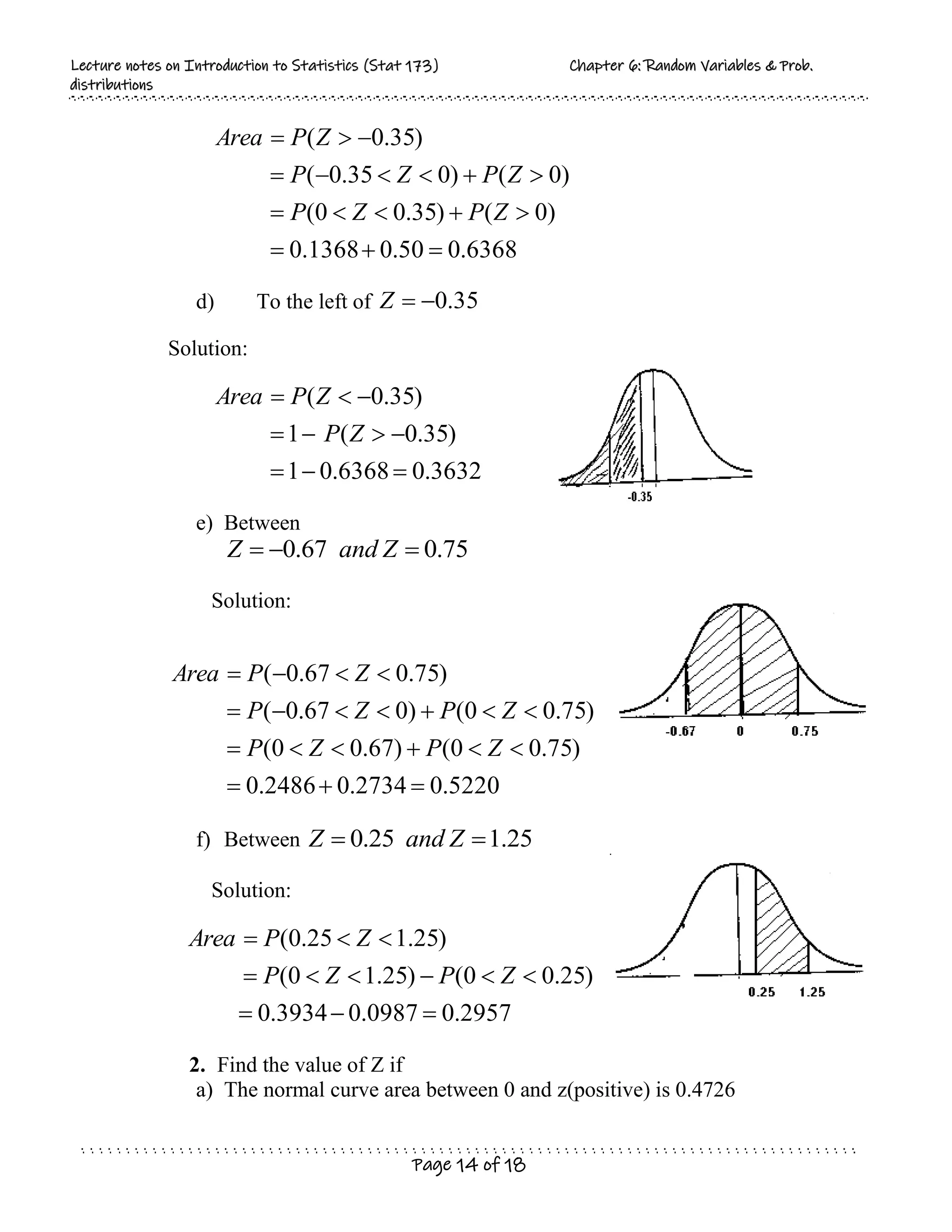
c) To the right of 35
.
0


Z
Solution:

L
Le
ec
ct
tu
ur
re
e n
no
ot
te
es
s o
on
n I
In
nt
tr
ro
od
du
uc
ct
ti
io
on
n t
to
o S
St
ta
at
ti
is
st
ti
ic
cs
s (
(S
St
ta
at
t 1
17
73
3)
) C
Ch
ha
ap
pt
te
er
r 6
6:
: R
Ra
an
nd
do
om
m V
Va
ar
ri
ia
ab
bl
le
es
s &
& P
Pr
ro
ob
b.
.
d
di
is
st
tr
ri
ib
bu
ut
ti
io
on
ns
s
Page 14 of 18
6368
.
0
50
.
0
1368
.
0
)
0
(
)
35
.
0
0
(
)
0
(
)
0
35
.
0
(
)
35
.
0
(

















Z
P
Z
P
Z
P
Z
P
Z
P
Area
d) To the left of 35
.
0


Z
Solution:
3632
.
0
6368
.
0
1
)
35
.
0
(
1
)
35
.
0
(










Z
P
Z
P
Area
e) Between
75
.
0
67
.
0 

 Z
and
Z
Solution:
5220
.
0
2734
.
0
2486
.
0
)
75
.
0
0
(
)
67
.
0
0
(
)
75
.
0
0
(
)
0
67
.
0
(
)
75
.
0
67
.
0
(




















Z
P
Z
P
Z
P
Z
P
Z
P
Area
f) Between 25
.
1
25
.
0 
 Z
and
Z
Solution:
2957
.
0
0987
.
0
3934
.
0
)
25
.
0
0
(
)
25
.
1
0
(
)
25
.
1
25
.
0
(












Z
P
Z
P
Z
P
Area
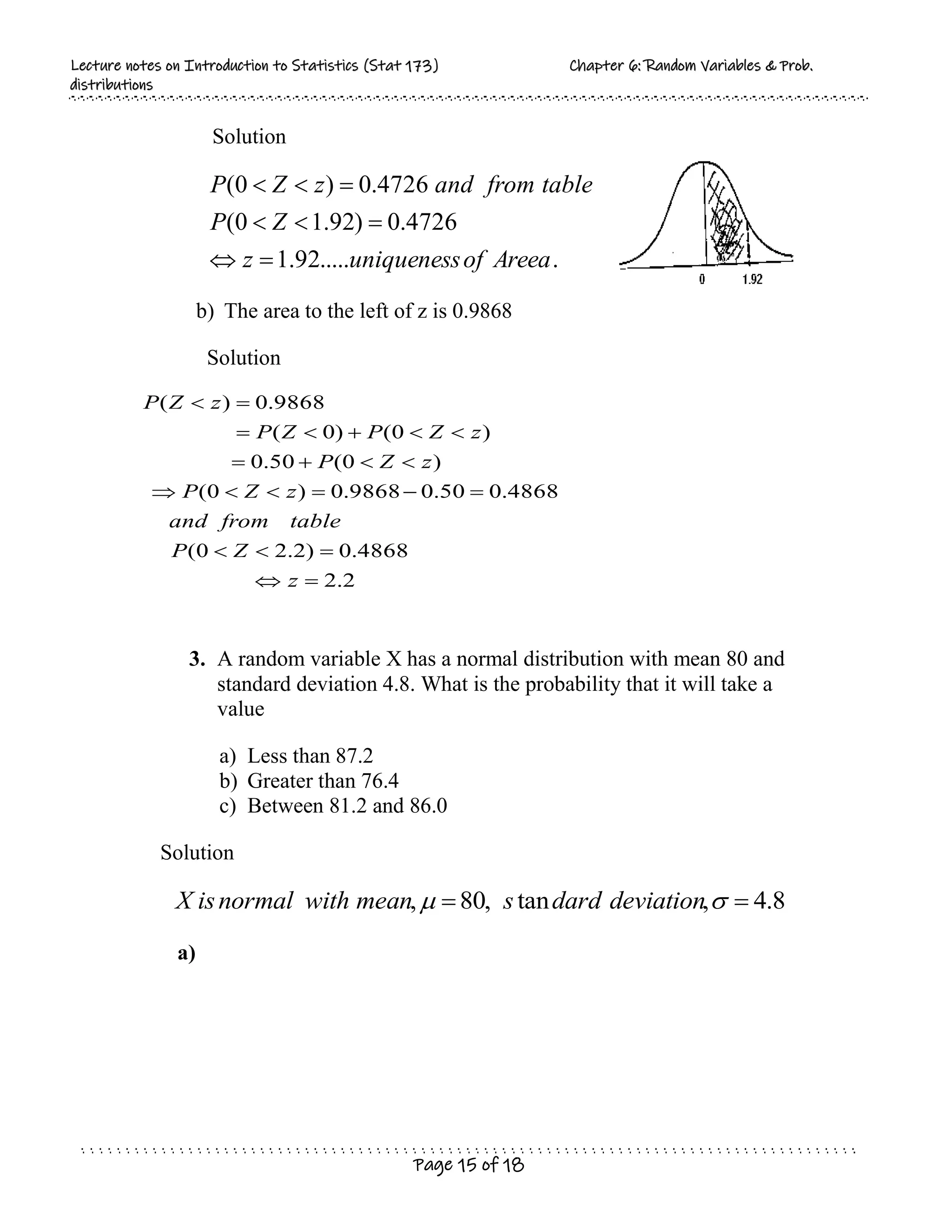
2. Find the value of Z if
a) The normal curve area between 0 and z(positive) is 0.4726

L
Le
ec
ct
tu
ur
re
e n
no
ot
te
es
s o
on
n I
In
nt
tr
ro
od
du
uc
ct
ti
io
on
n t
to
o S
St
ta
at
ti
is
st
ti
ic
cs
s (
(S
St
ta
at
t 1
17
73
3)
) C
Ch
ha
ap
pt
te
er
r 6
6:
: R
Ra
an
nd
do
om
m V
Va
ar
ri
ia
ab
bl
le
es
s &
& P
Pr
ro
ob
b.
.
d
di
is
st
tr
ri
ib
bu
ut
ti
io
on
ns
s
Page 15 of 18
Solution
.
.....
92
.
1
4726
.
0
)
92
.
1
0
(
4726
.
0
)
0
(
Areea
of
uniqueness
z
Z
P
table
from
and
z
Z
P








b) The area to the left of z is 0.9868
Solution
2
.
2
4868
.
0
)
2
.
2
0
(
4868
.
0
50
.
0
9868
.
0
)
0
(
)
0
(
50
.
0
)
0
(
)
0
(
9868
.
0
)
(






















z
Z
P
table
from
and
z
Z
P
z
Z
P
z
Z
P
Z
P
z
Z
P
3. A random variable X has a normal distribution with mean 80 and
standard deviation 4.8. What is the probability that it will take a
value
a) Less than 87.2
b) Greater than 76.4
c) Between 81.2 and 86.0
Solution
8
.
4
,
tan
,
80
, 
 
 deviation
dard
s
mean
with
normal
is
X
a)

L
Le
ec
ct
tu
ur
re
e n
no
ot
te
es
s o
on
n I
In
nt
tr
ro
od
du
uc
ct
ti
io
on
n t
to
o S
St
ta
at
ti
is
st
ti
ic
cs
s (
(S
St
ta
at
t 1
17
73
3)
) C
Ch
ha
ap
pt
te
er
r 6
6:
: R
Ra
an
nd
do
om
m V
Va
ar
ri
ia
ab
bl
le
es
s &
& P
Pr
ro
ob
b.
.
d
di
is
st
tr
ri
ib
bu
ut
ti
io
on
ns
s
Page 16 of 18
9332
.
0
4332
.
0
50
.
0
)
5
.
1
0
(
)
0
(
)
5
.
1
(
)
8
.
4
80
2
.
87
(
)
2
.
87
(
)
2
.
87
(


















Z
P
Z
P
Z
P
Z
P
X
P
X
P




b)
7734
.
0
2734
.
0
50
.
0
)
75
.
0
0
(
)
0
(
)
75
.
0
(
)
8
.
4
80
4
.
76
(
)
4
.
76
(
)
4
.
76
(



















Z
P
Z
P
Z
P
Z
P
X
P
X
P




c)
2957
.
0
0987
.
0
3934
.
0
)
25
.
1
0
(
)
25
.
1
0
(
)
25
.
1
25
.
0
(
)
8
.
4
80
0
.
86
8
.
4
80
2
.
81
(
)
0
.
86
2
.
81
(
)
0
.
86
2
.
81
(

























Z
P
Z
P
Z
P
Z
P
X
P
X
P






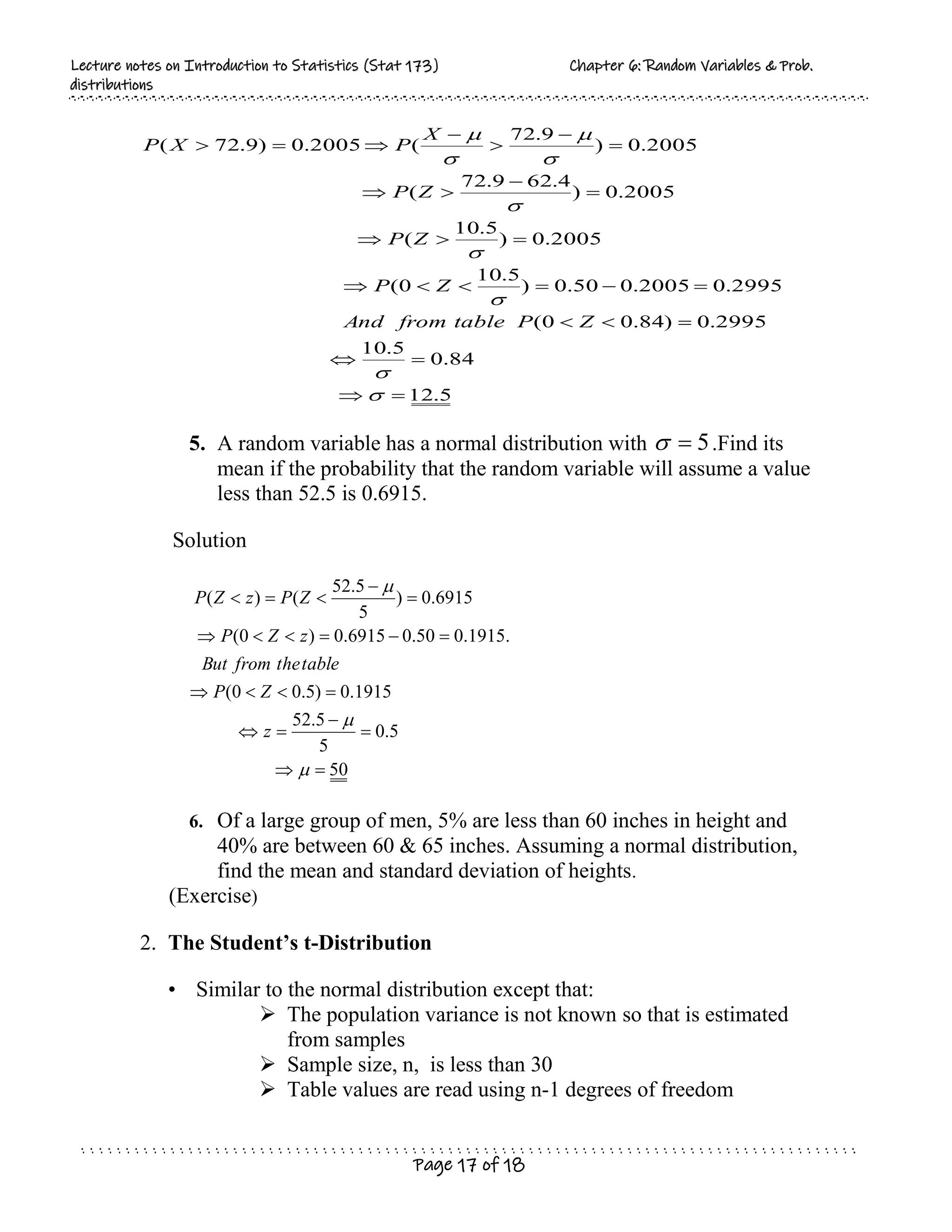
4. A normal distribution has mean 62.4.Find its standard deviation if
20.0% of the area under the normal curve lies to the right of 72.9
Solution

L
Le
ec
ct
tu
ur
re
e n
no
ot
te
es
s o
on
n I
In
nt
tr
ro
od
du
uc
ct
ti
io
on
n t
to
o S
St
ta
at
ti
is
st
ti
ic
cs
s (
(S
St
ta
at
t 1
17
73
3)
) C
Ch
ha
ap
pt
te
er
r 6
6:
: R
Ra
an
nd
do
om
m V
Va
ar
ri
ia
ab
bl
le
es
s &
& P
Pr
ro
ob
b.
.
d
di
is
st
tr
ri
ib
bu
ut
ti
io
on
ns
s
Page 17 of 18
5
.
12
84
.
0
5
.
10
2995
.
0
)
84
.
0
0
(
2995
.
0
2005
.
0
50
.
0
)
5
.
10
0
(
2005
.
0
)
5
.
10
(
2005
.
0
)
4
.
62
9
.
72
(
2005
.
0
)
9
.
72
(
2005
.
0
)
9
.
72
(




































Z
P
table
from
And
Z
P
Z
P
Z
P
X
P
X
P
5. A random variable has a normal distribution with 5

 .Find its
mean if the probability that the random variable will assume a value
less than 52.5 is 0.6915.
Solution
50
5
.
0
5
5
.
52
1915
.
0
)
5
.
0
0
(
.
1915
.
0
50
.
0
6915
.
0
)
0
(
6915
.
0
)
5
5
.
52
(
)
(
























z
Z
P
table
the
from
But
z
Z
P
Z
P
z
Z
P
6. Of a large group of men, 5% are less than 60 inches in height and
40% are between 60 & 65 inches. Assuming a normal distribution,
find the mean and standard deviation of heights.
(Exercise)
2. The Student’s t-Distribution
• Similar to the normal distribution except that:
 The population variance is not known so that is estimated
from samples
 Sample size, n, is less than 30
 Table values are read using n-1 degrees of freedom

L
Le
ec
ct
tu
ur
re
e n
no
ot
te
es
s o
on
n I
In
nt
tr
ro
od
du
uc
ct
ti
io
on
n t
to
o S
St
ta
at
ti
is
st
ti
ic
cs
s (
(S
St
ta
at
t 1
17
73
3)
) C
Ch
ha
ap
pt
te
er
r 6
6:
: R
Ra
an
nd
do
om
m V
Va
ar
ri
ia
ab
bl
le
es
s &
& P
Pr
ro
ob
b.
.
d
di
is
st
tr
ri
ib
bu
ut
ti
io
on
ns
s
Page 18 of 18
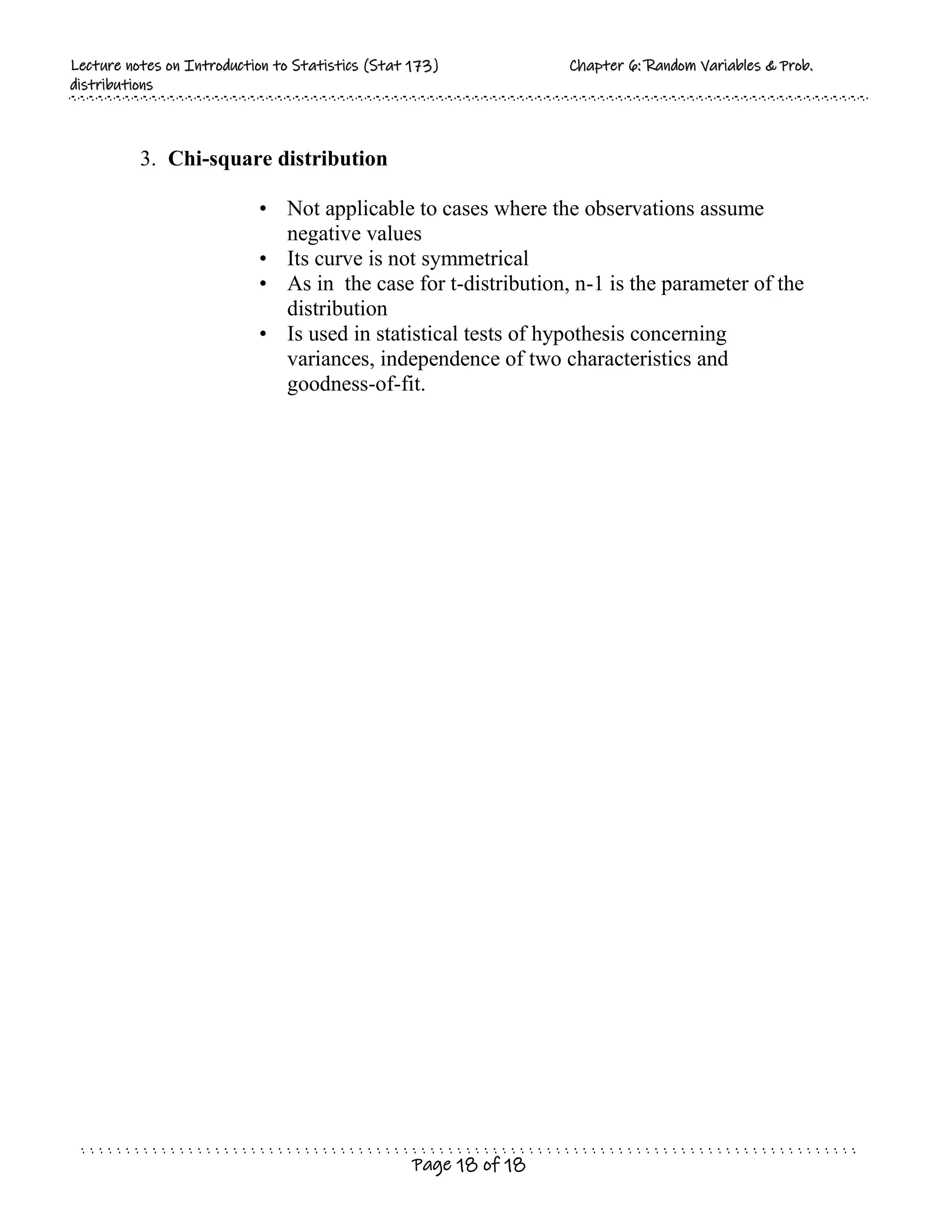
3. Chi-square distribution
• Not applicable to cases where the observations assume
negative values
• Its curve is not symmetrical
• As in the case for t-distribution, n-1 is the parameter of the
distribution
• Is used in statistical tests of hypothesis concerning
variances, independence of two characteristics and
goodness-of-fit.

Chapter-6-Random Variables & Probability distributions-3.doc

In this document

More Related Content

What's hot

Similar to Chapter-6-Random Variables & Probability distributions-3.doc

More from BULE HORA UNIVERSITY(DESALE CHALI)

Recently uploaded

Chapter-6-Random Variables & Probability distributions-3.doc