Syllabus
• Trees -Binary Trees, Binary Search Trees, AVL
Trees, 2-4 trees, Hash tables, tries.
• Binary Trees and Binary Search Trees -
Operations, Representation, Traversals. Hash
tables - concept of hashing, hash function,
collision and collision resolution.
3.
Linear Data Structures
•Arrays, linked lists, stacks and queues were
examples of linear data structures in which
elements are arranged in a linear fashion (ie,
one dimensional representation).
4.
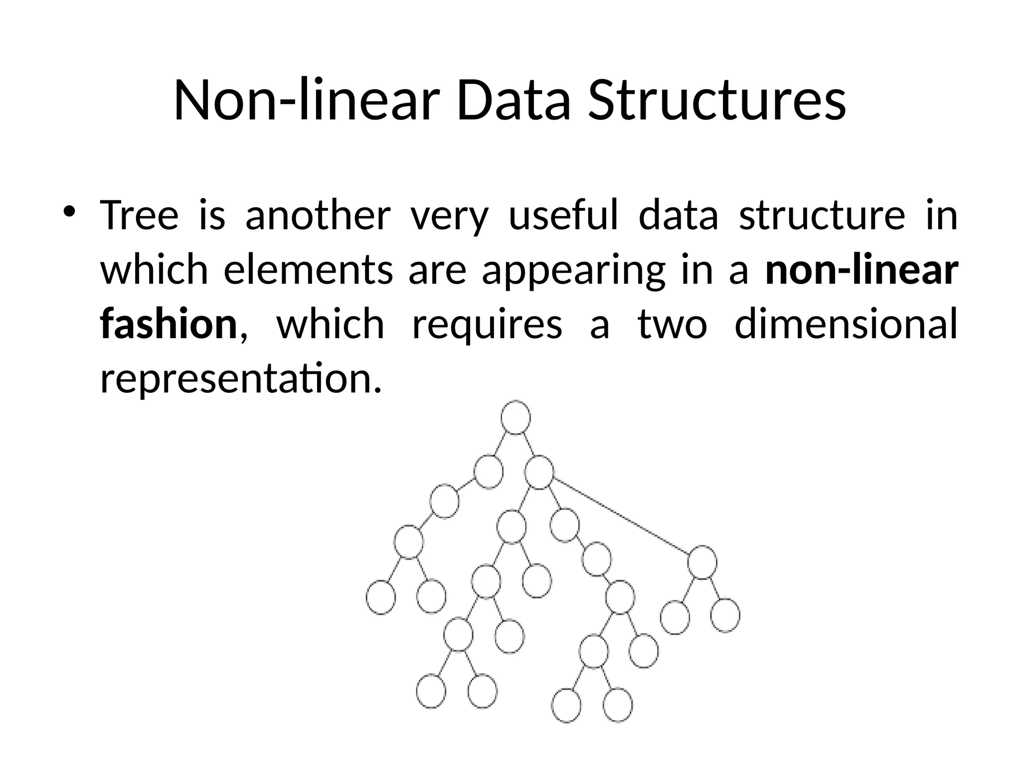
Non-linear Data Structures
•Tree is another very useful data structure in
which elements are appearing in a non-linear
fashion, which requires a two dimensional
representation.
5.
Tree
Tree isa nonlinear data structure
The elements appear in a non linear fashion, which
require two dimensional representations.
Using tree it is easy to organize hierarchical
representation of objects.
Tree is efficient for maintaining and manipulating
data, where the hierarchy of relationship among the
data is to be preserved.
6.
Tree
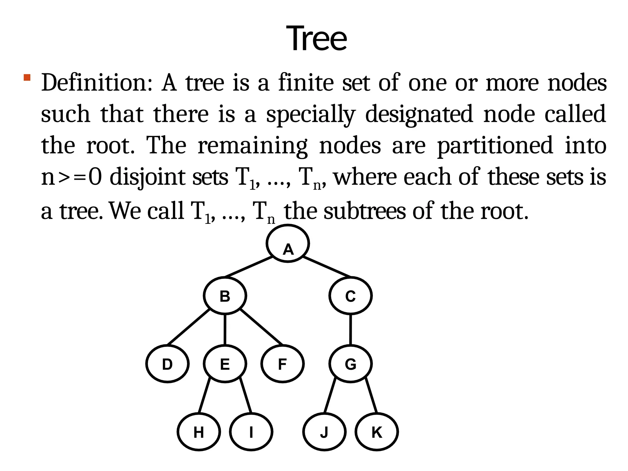
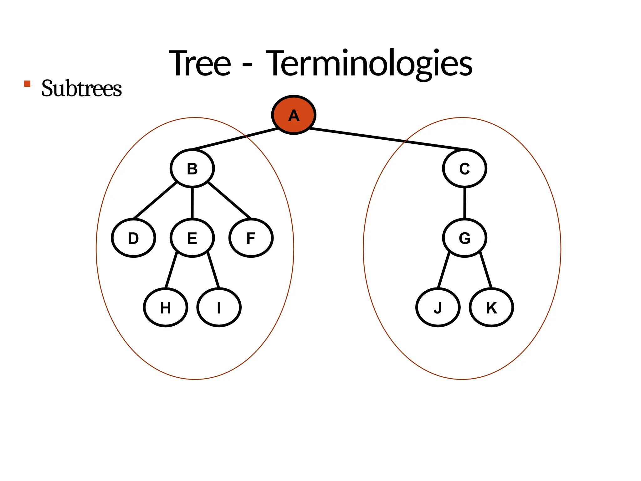
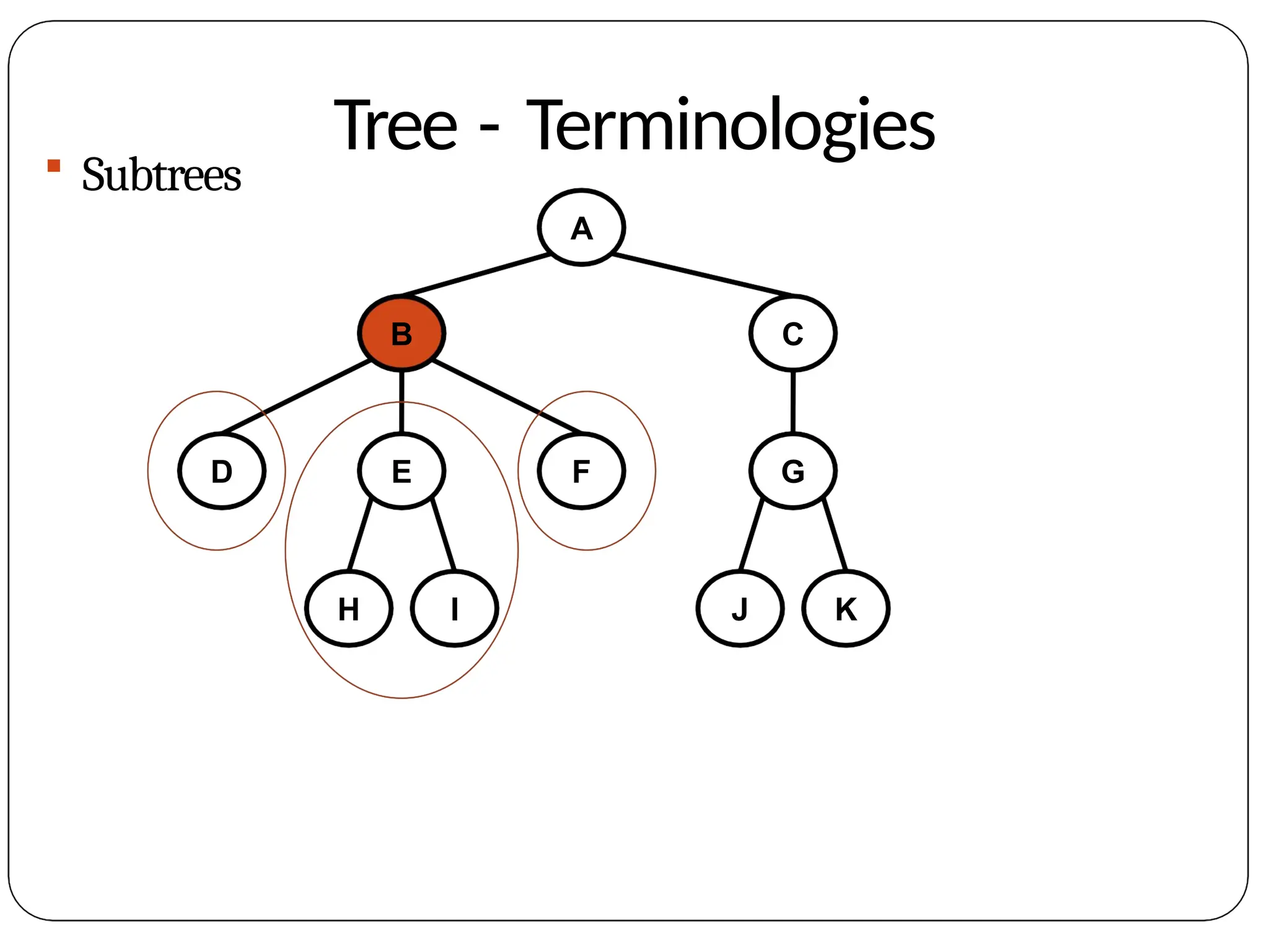
Definition: Atree is a finite set of one or more nodes
such that there is a specially designated node called
the root. The remaining nodes are partitioned into
n>=0 disjoint sets T1, ..., Tn, where each of these sets is
a tree. We call T1, ..., Tn the subtrees of the root.
A
B C
D E F G
H I J K
7.
Tree - Terminologies
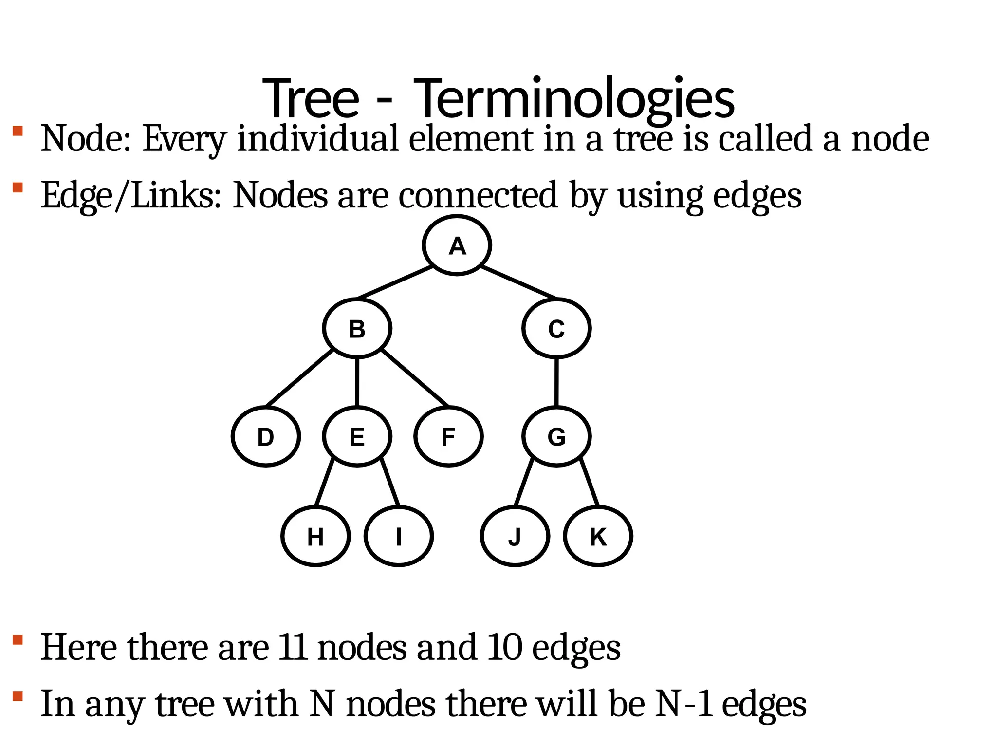
Here there are 11 nodes and 10 edges
In any tree with N nodes there will be N-1 edges
Node: Every individual element in a tree is called a node
Edge/Links: Nodes are connected by using edges
A
B C
D E F G
H I J K
8.
Tree - Terminologies
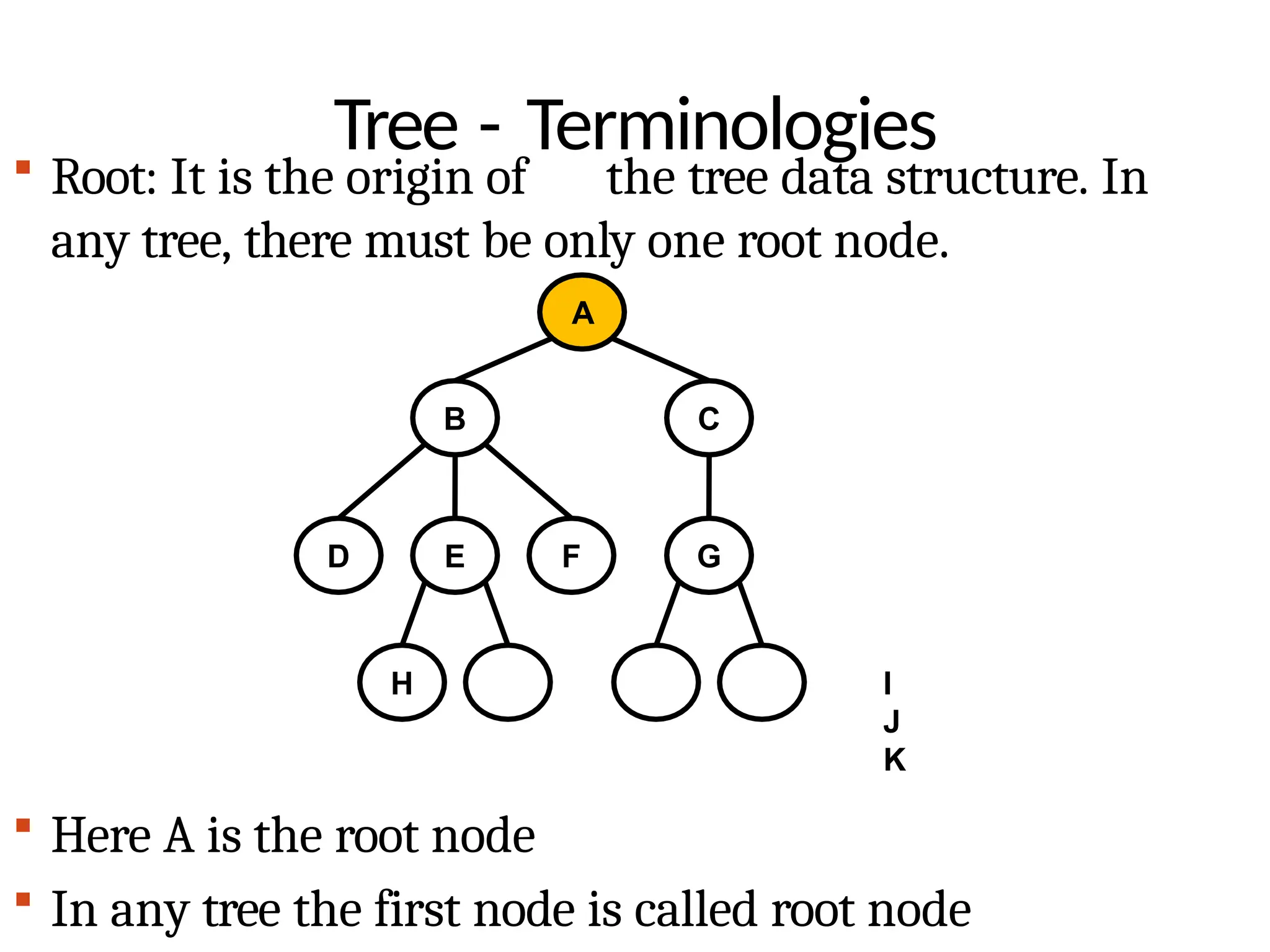
Root: It is the origin of the tree data structure. In
any tree, there must be only one root node.
A
B C
D E F G
H I
J
K
Here A is the root node
In any tree the first node is called root node
9.
Tree - Terminologies
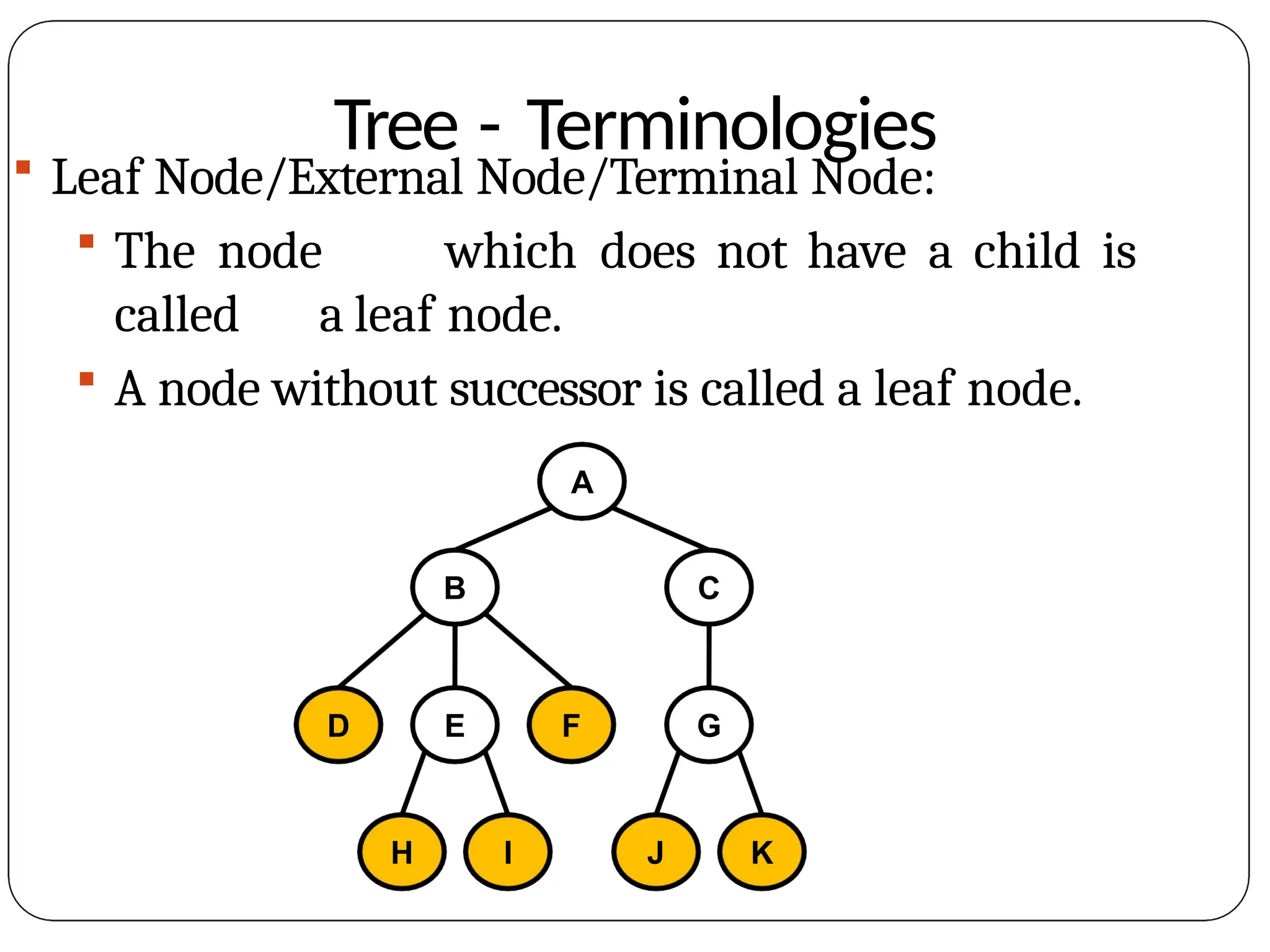
Leaf Node/External Node/Terminal Node:
The node which does not have a child is
called a leaf node.
A node without successor is called a leaf node.
A
B C
D E F G
H I J K
10.
Tree - Terminologies
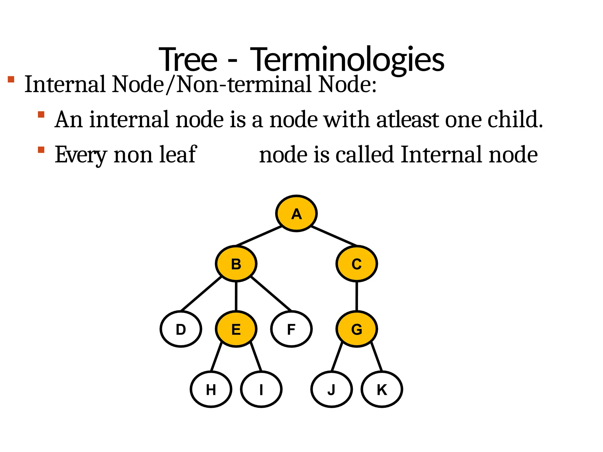
Internal Node/Non-terminal Node:
An internal node is a node with atleast one child.
Every non leaf node is called Internal node
A
B C
D E F G
H I J K
11.
Tree - Terminologies
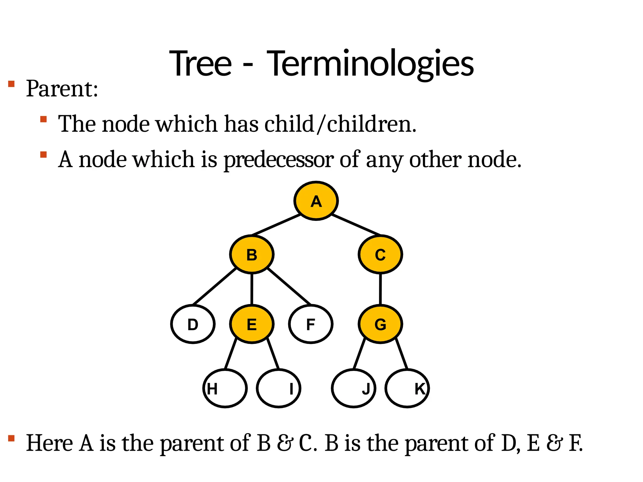
Parent:
The node which has child/children.
A node which is predecessor of any other node.
A
B C
D E F G
H I J K
Here A is the parent of B & C. B is the parent of D, E & F.
12.
Tree - Terminologies
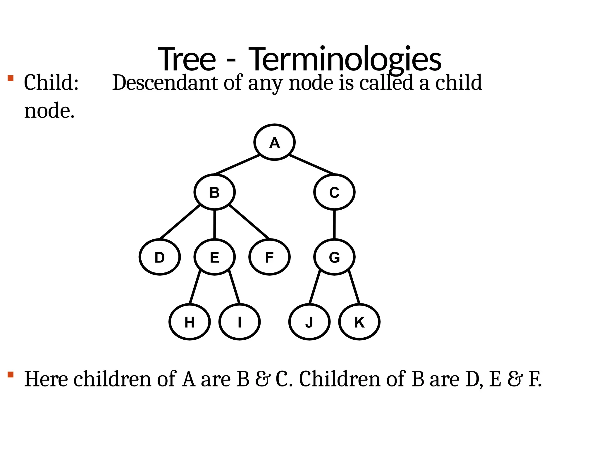
Child: Descendant of any node is called a child
node.
Here children of A are B & C. Children of B are D, E & F.
A
B C
D E F G
H I J K
13.
Order of
nodes
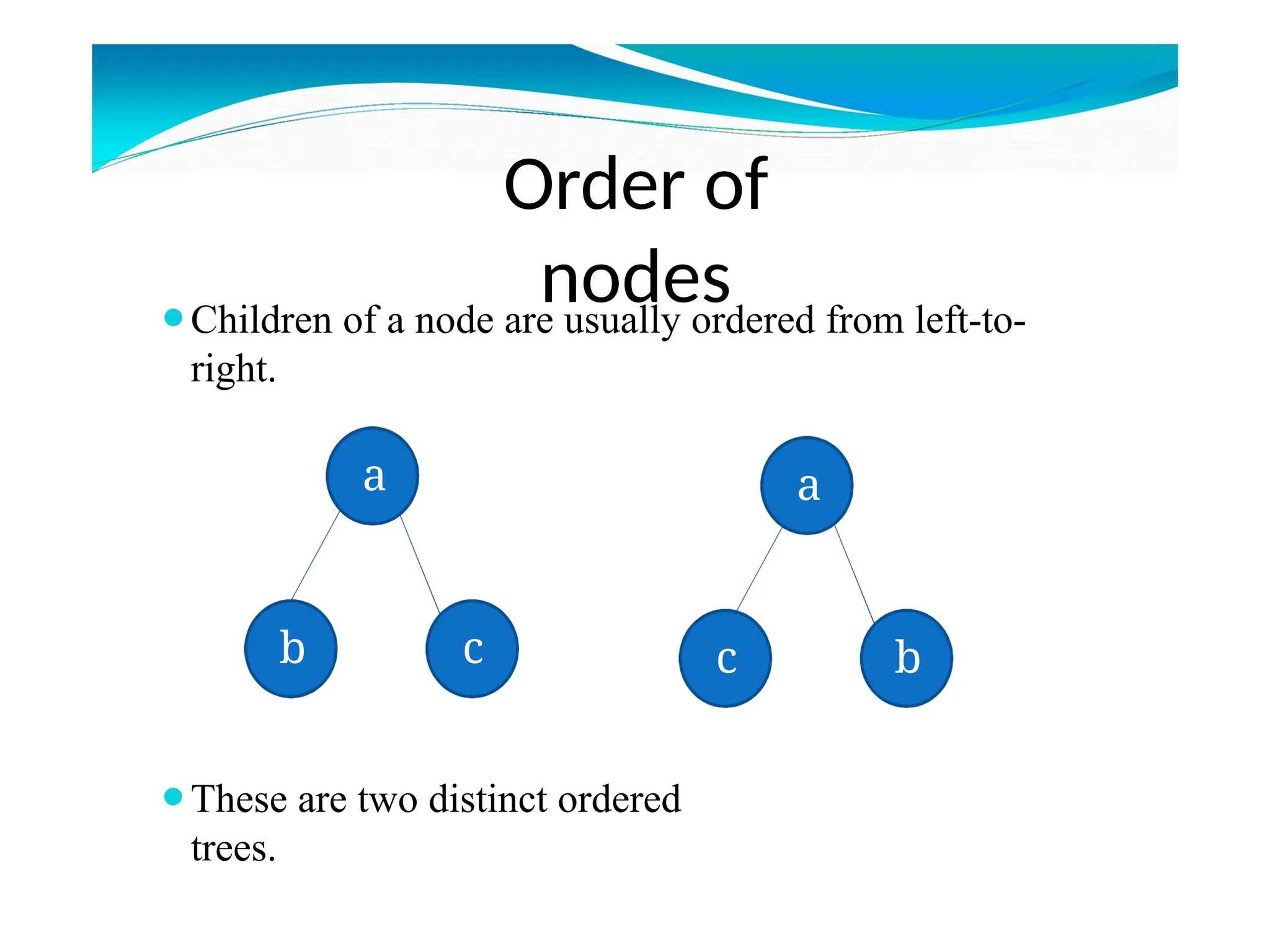
⚫Children ofa node are usually ordered from left-to-
right.
⚫These are two distinct ordered
trees.
a
b c
a
c b
14.
⚫If a andb are siblings, and a is to the left of b, then all
the descendants of a are to the left of all descendants of
b.
⚫A tree in which the order of nodes is ignored is referred
to as unordered tree.
15.
Tree - Terminologies
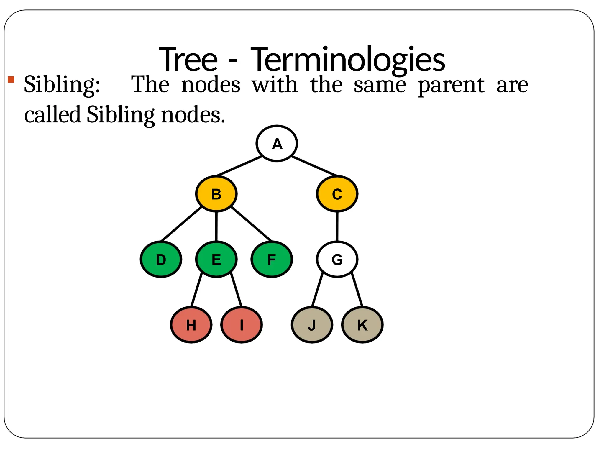
Sibling: The nodes with the same parent are
called Sibling nodes.
A
B C
D E F G
H I J K
16.
Tree - Terminologies
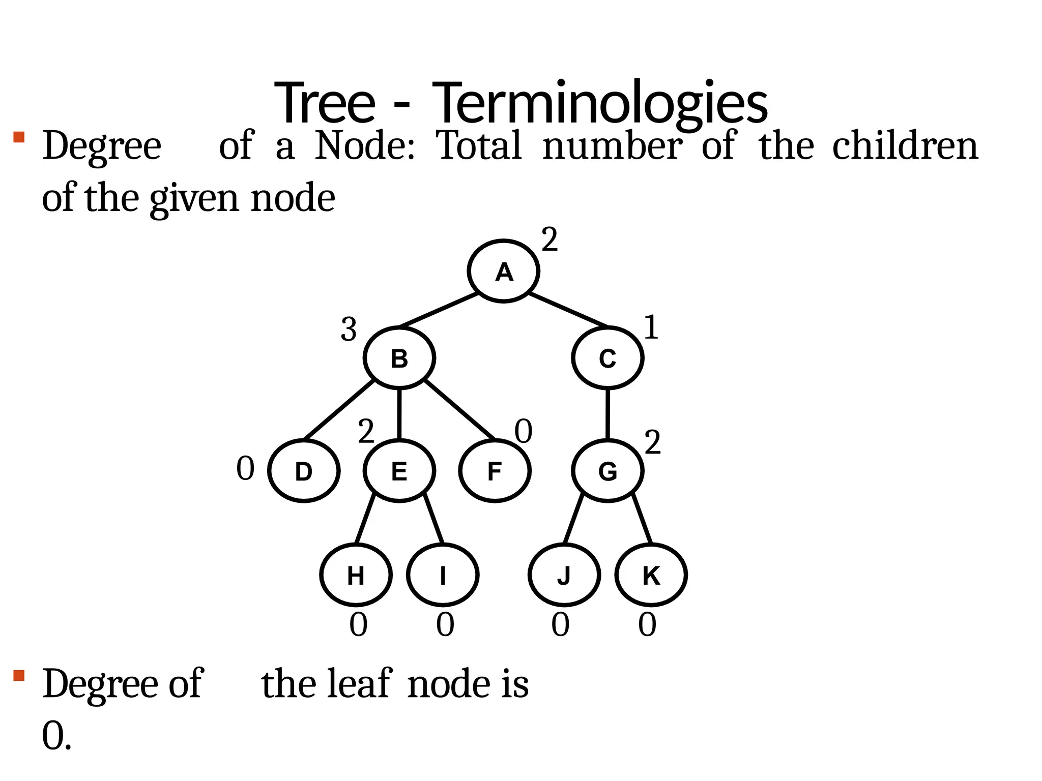
Degree of the leaf node is
0.
B C
D G
Degree of a Node: Total number of the children
of the given node
2
A
3 1
2
J
0
K
0
0
2
E
0
F
H
0
I
0
17.
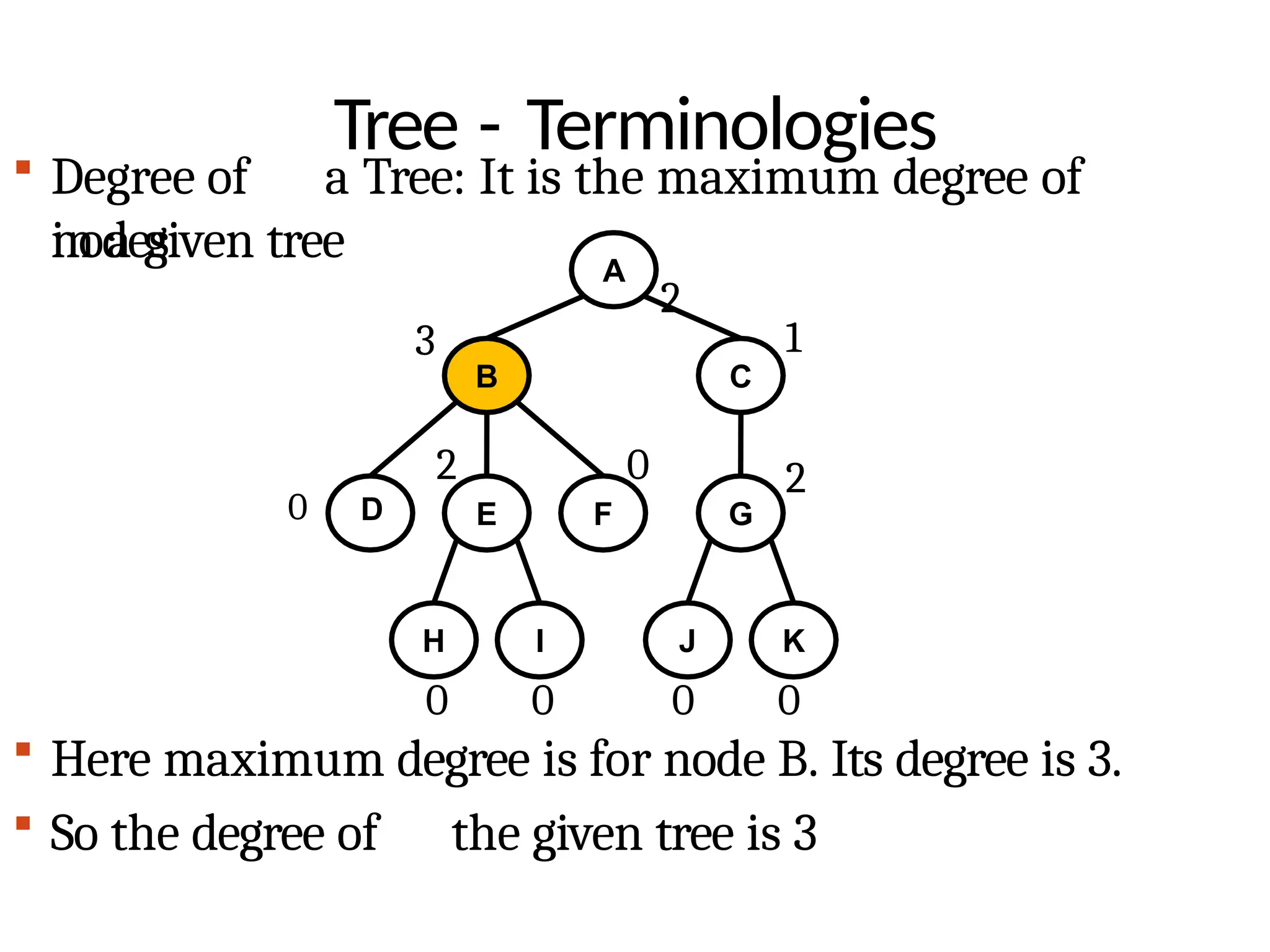
Tree - Terminologies
ina given tree
Here maximum degree is for node B. Its degree is 3.
So the degree of the given tree is 3
A
B C
G
Degree of a Tree: It is the maximum degree of
nodes
2
3 1
2
J
0
K
0
0 D
2
E
0
F
H
0
I
0
18.
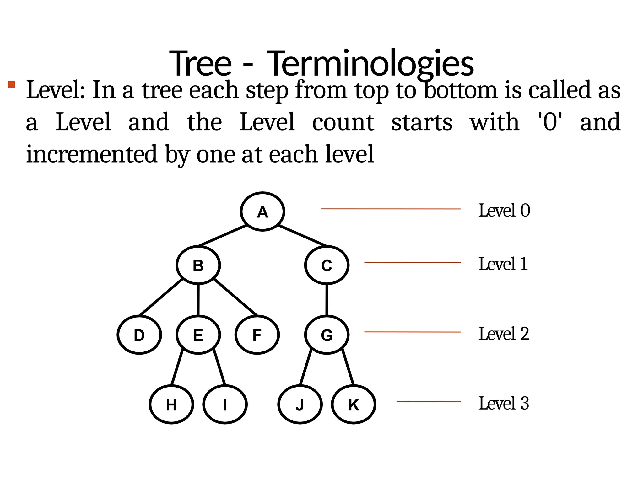
Tree - Terminologies
Level: In a tree each step from top to bottom is called as
a Level and the Level count starts with '0' and
incremented by one at each level
A
B C
D E F G
H I J K
Level 0
Level 1
Level 2
Level 3
19.
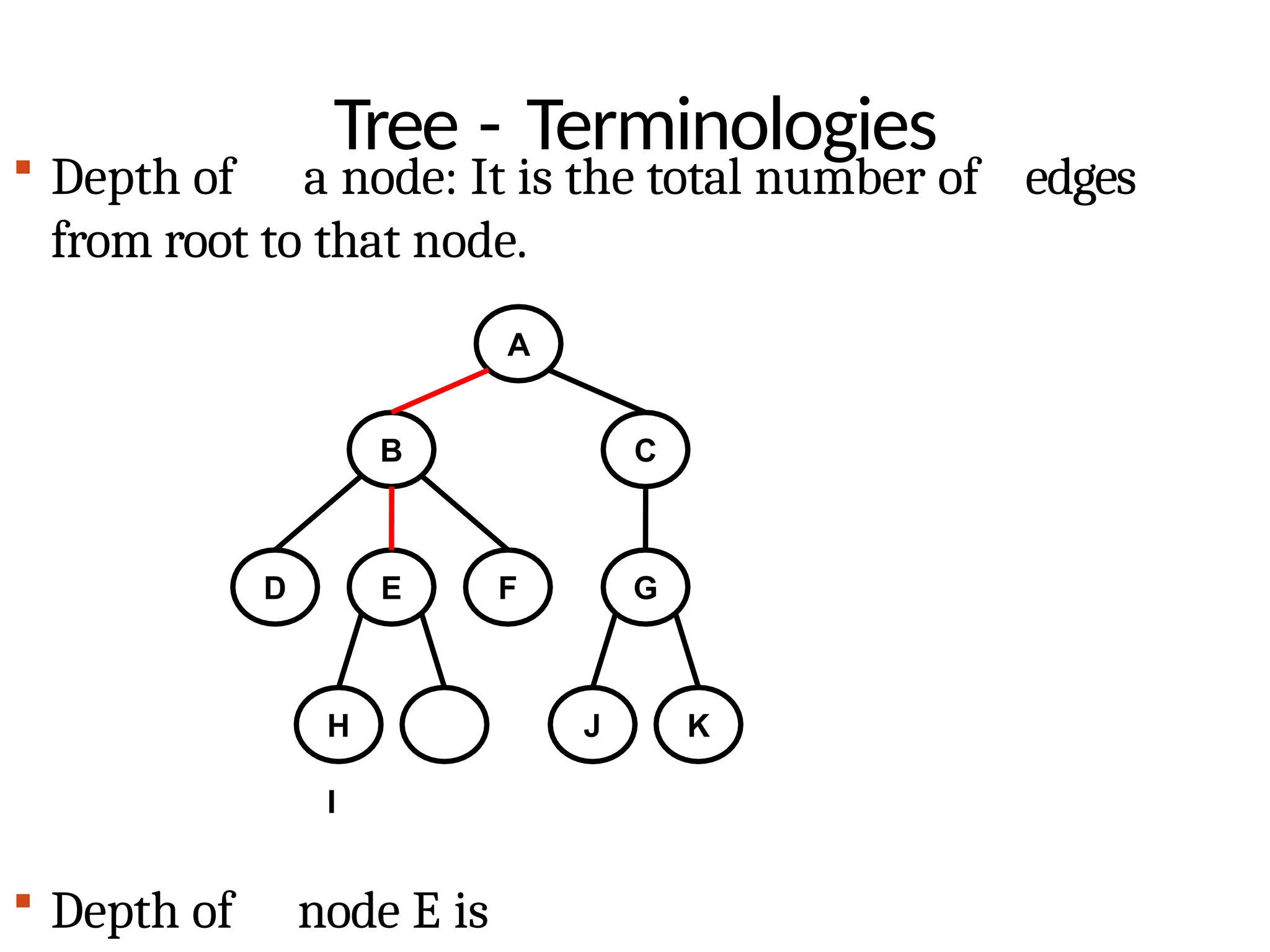
Tree - Terminologies
Depth of a node: It is the total number of edges
from root to that node.
A
B C
D E F G
H
I
Depth of node E is
J K
20.
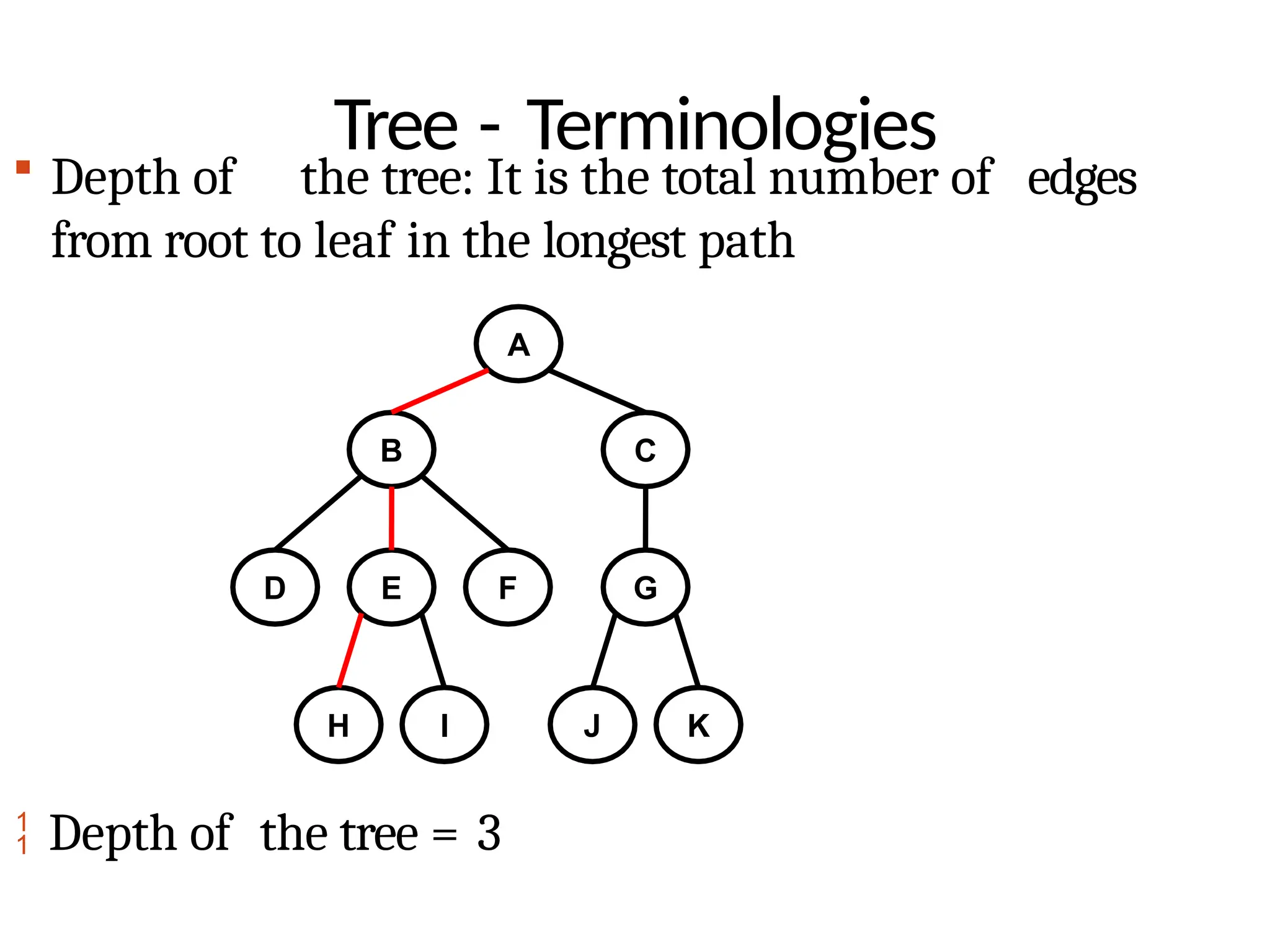
Tree - Terminologies
Depth of the tree: It is the total number of edges
from root to leaf in the longest path
A
B C
D E F G
H I J K
Depth of the tree = 3
21.
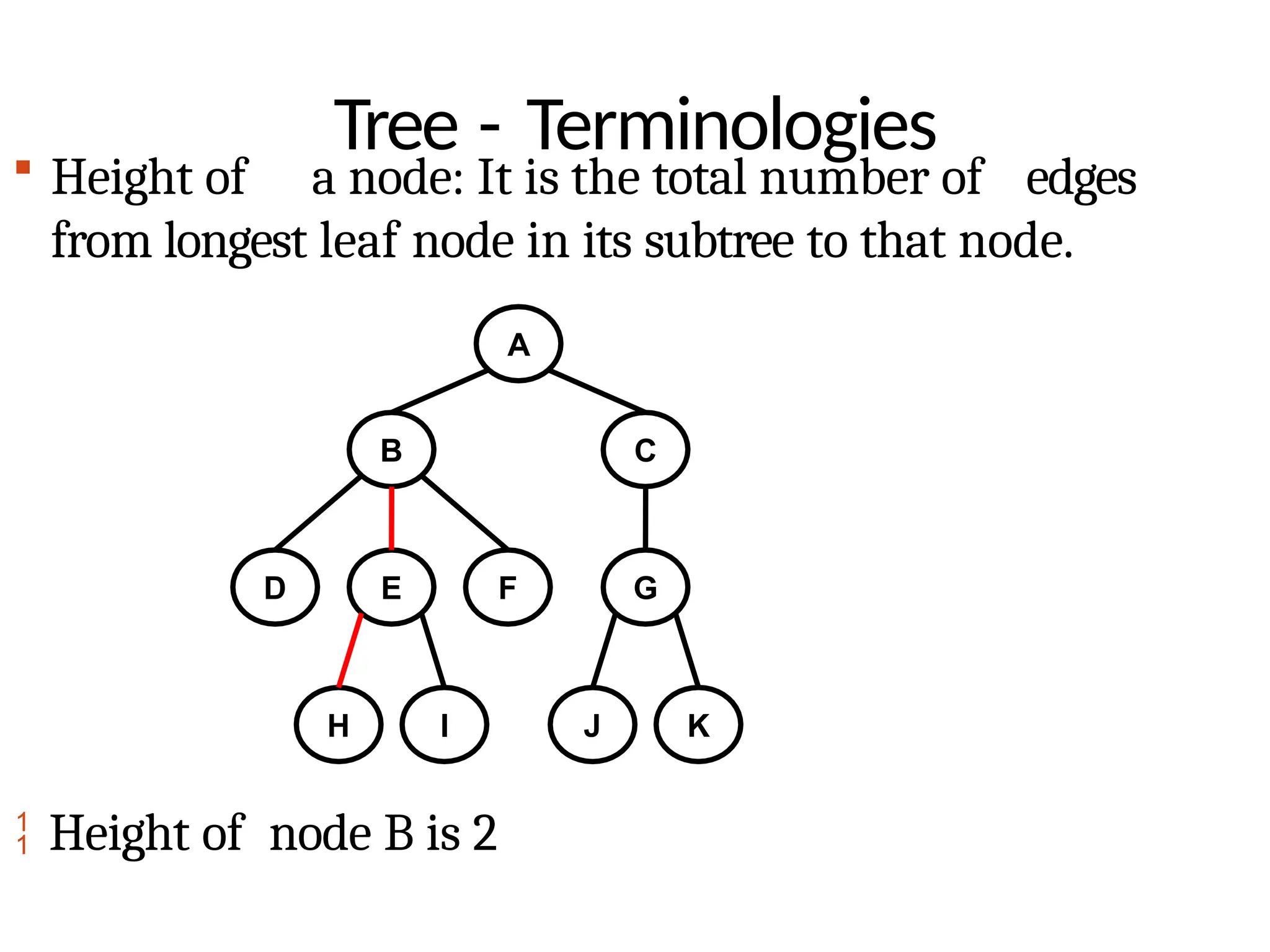
Tree - Terminologies
Height of a node: It is the total number of edges
from longest leaf node in its subtree to that node.
A
B C
D E F G
H I J K
Height of node B is 2
22.
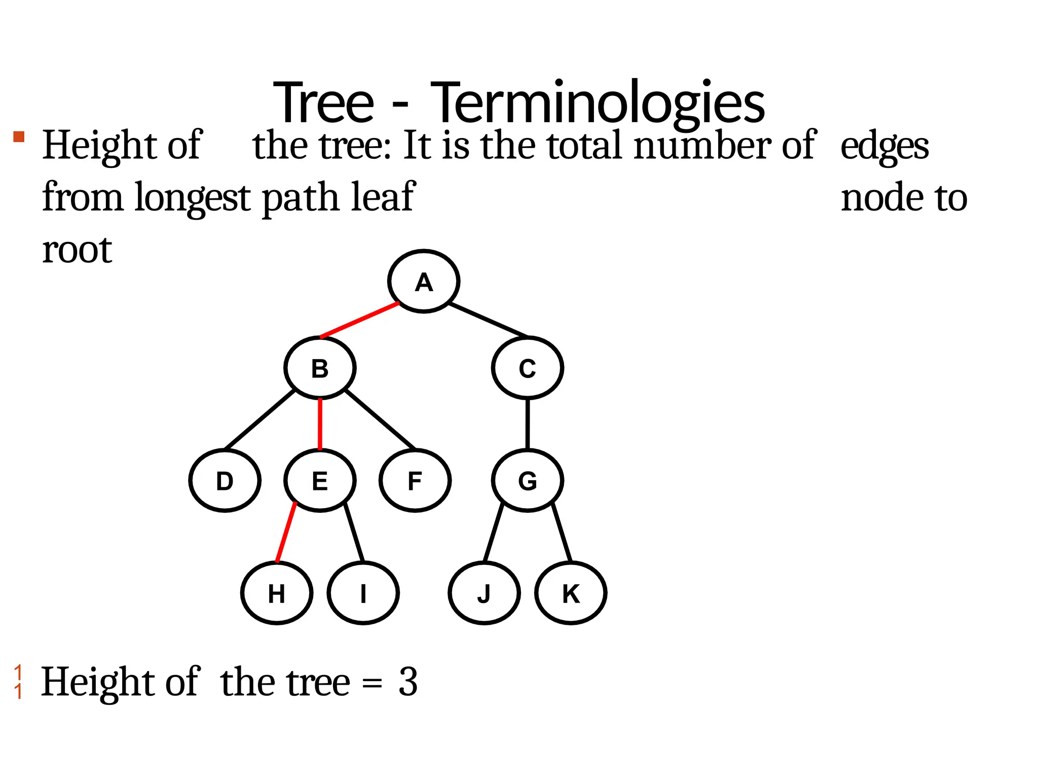
Tree - Terminologies
Height of the tree: It is the total number of edges
from longest path leaf node to
root
A
B C
D E F G
H I J K
Height of the tree = 3
23.
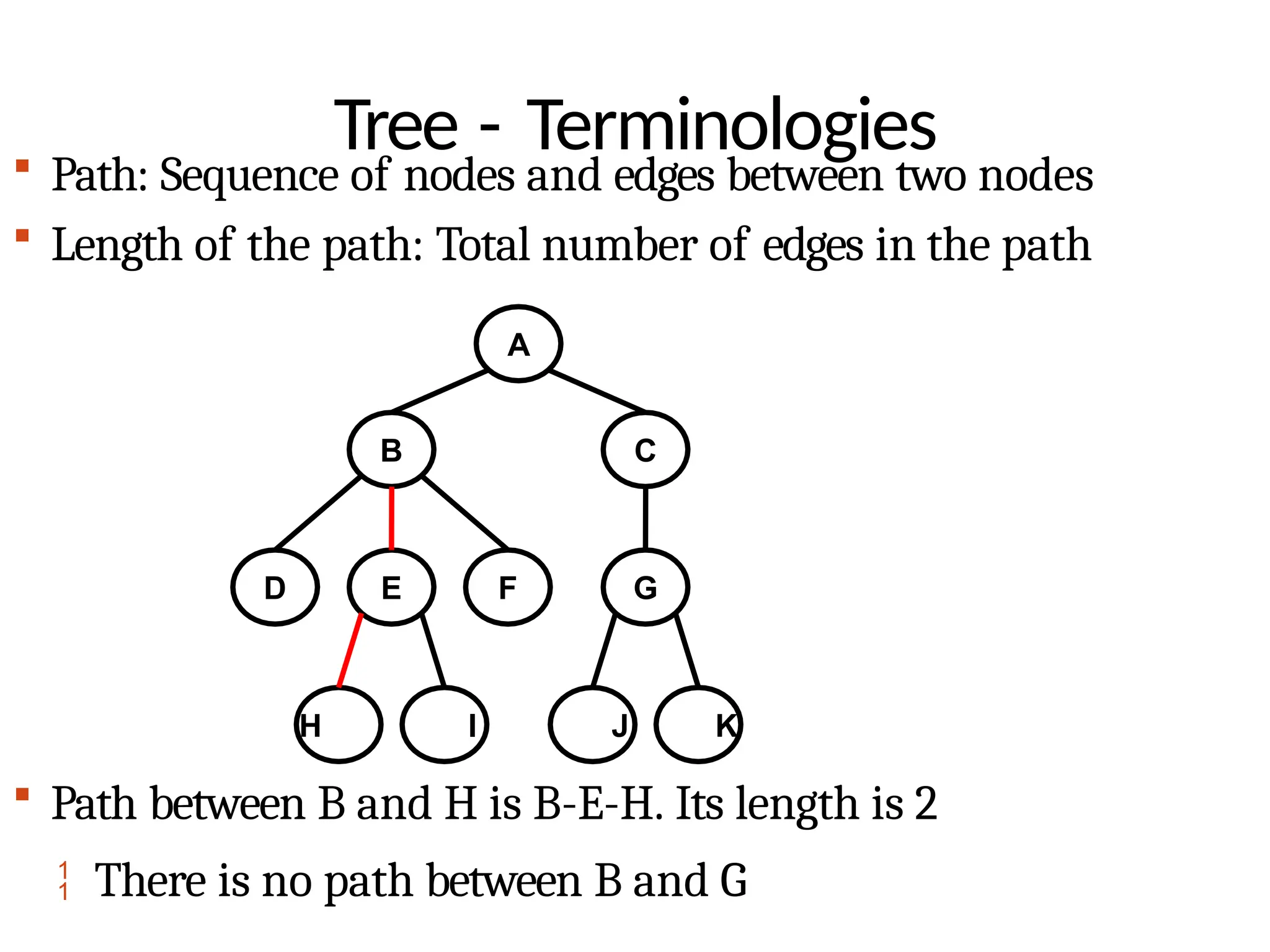
Tree - Terminologies
Path: Sequence of nodes and edges between two nodes
Length of the path: Total number of edges in the path
A
B C
D E F G
H I J K
Path between B and H is B-E-H. Its length is 2
There is no path between B and G
24.
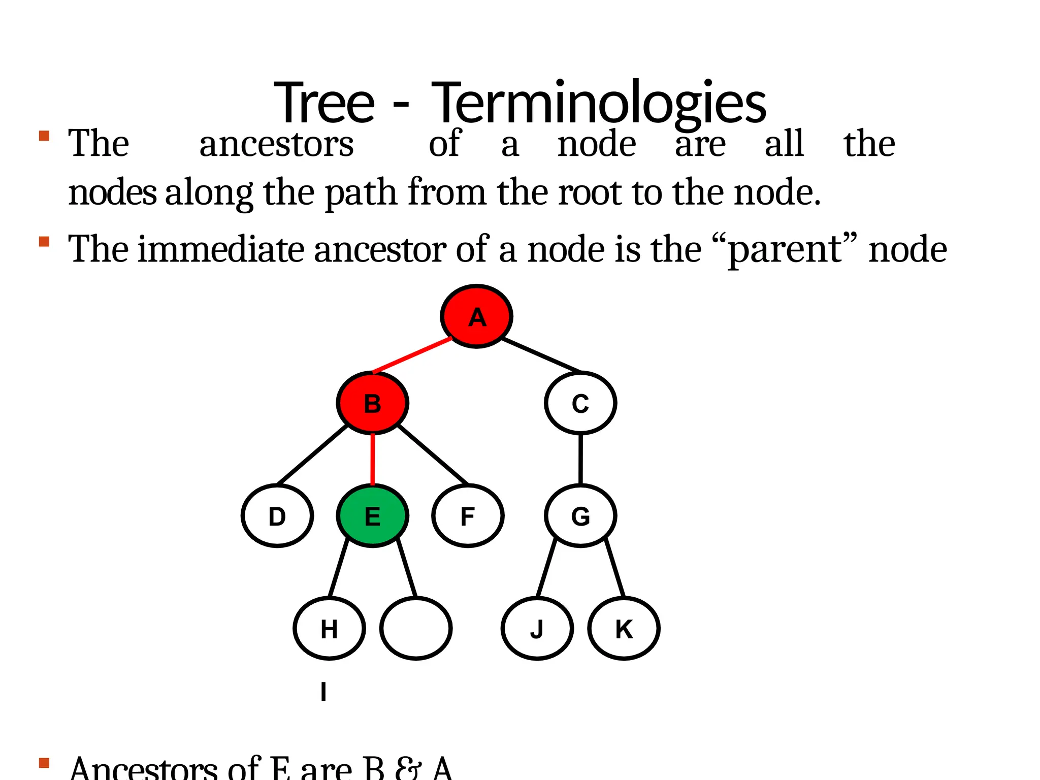
Tree - Terminologies
The ancestors of a node are all the
nodes along the path from the root to the node.
The immediate ancestor of a node is the “parent” node
A
B C
D E F G
H
I
J K
25.
Tree - Terminologies
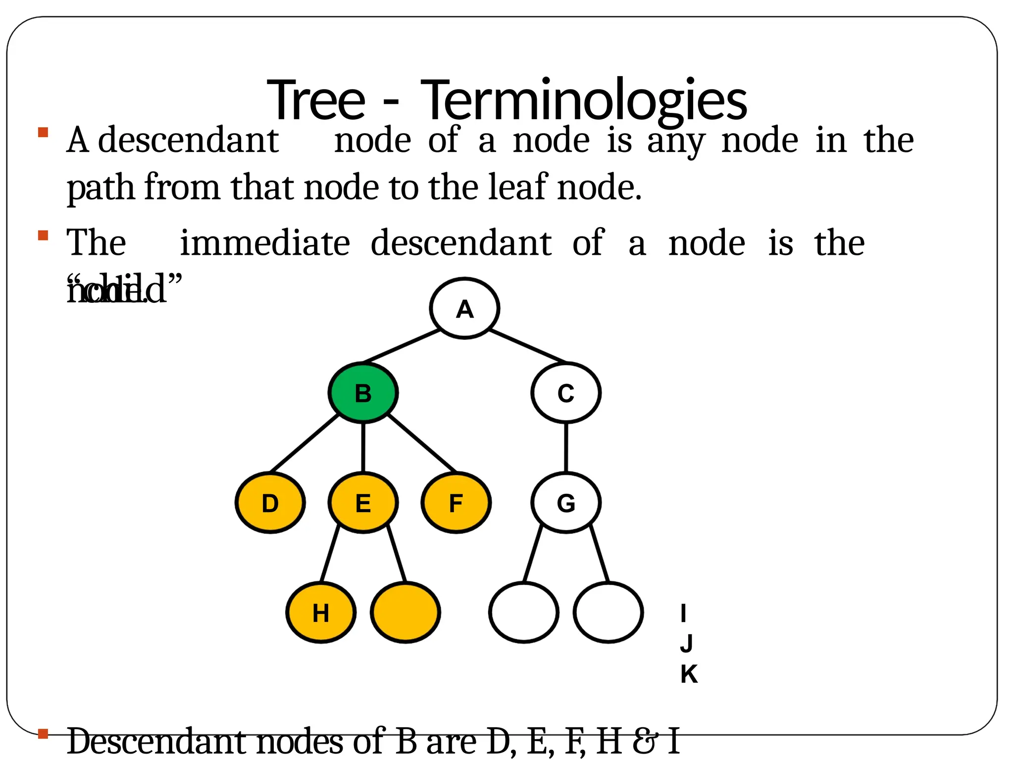
A descendant node of a node is any node in the
path from that node to the leaf node.
The immediate descendant of a node is the
“child”
node. A
B C
D E F G
H I
J
K
Descendant nodes of B are D, E, F, H & I
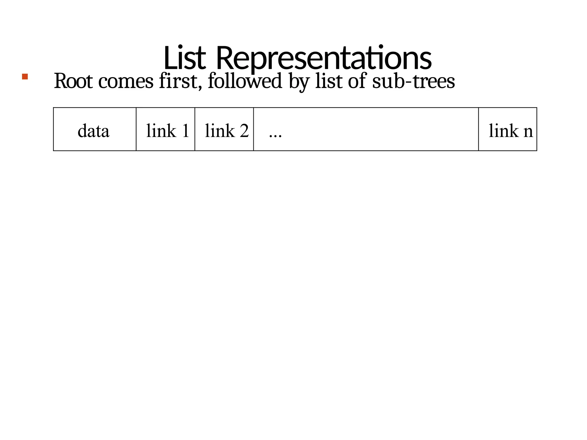
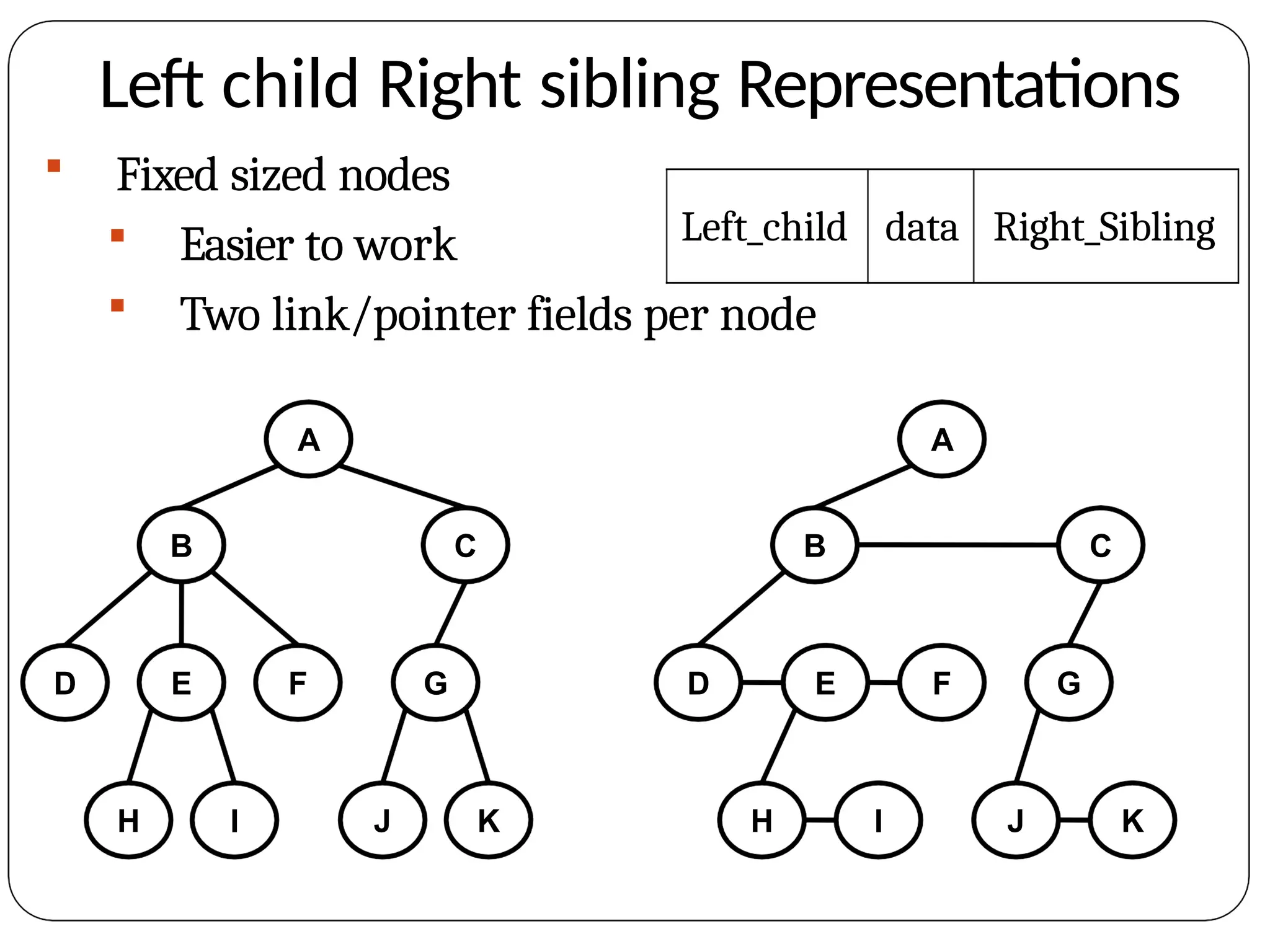
Left child Rightsibling Representations
Fixed sized nodes
Easier to work
Two link/pointer fields per node
A
B C
D E F G
H I J K
A
B C
D E F G
H I J K
Left_child data Right_Sibling
31.
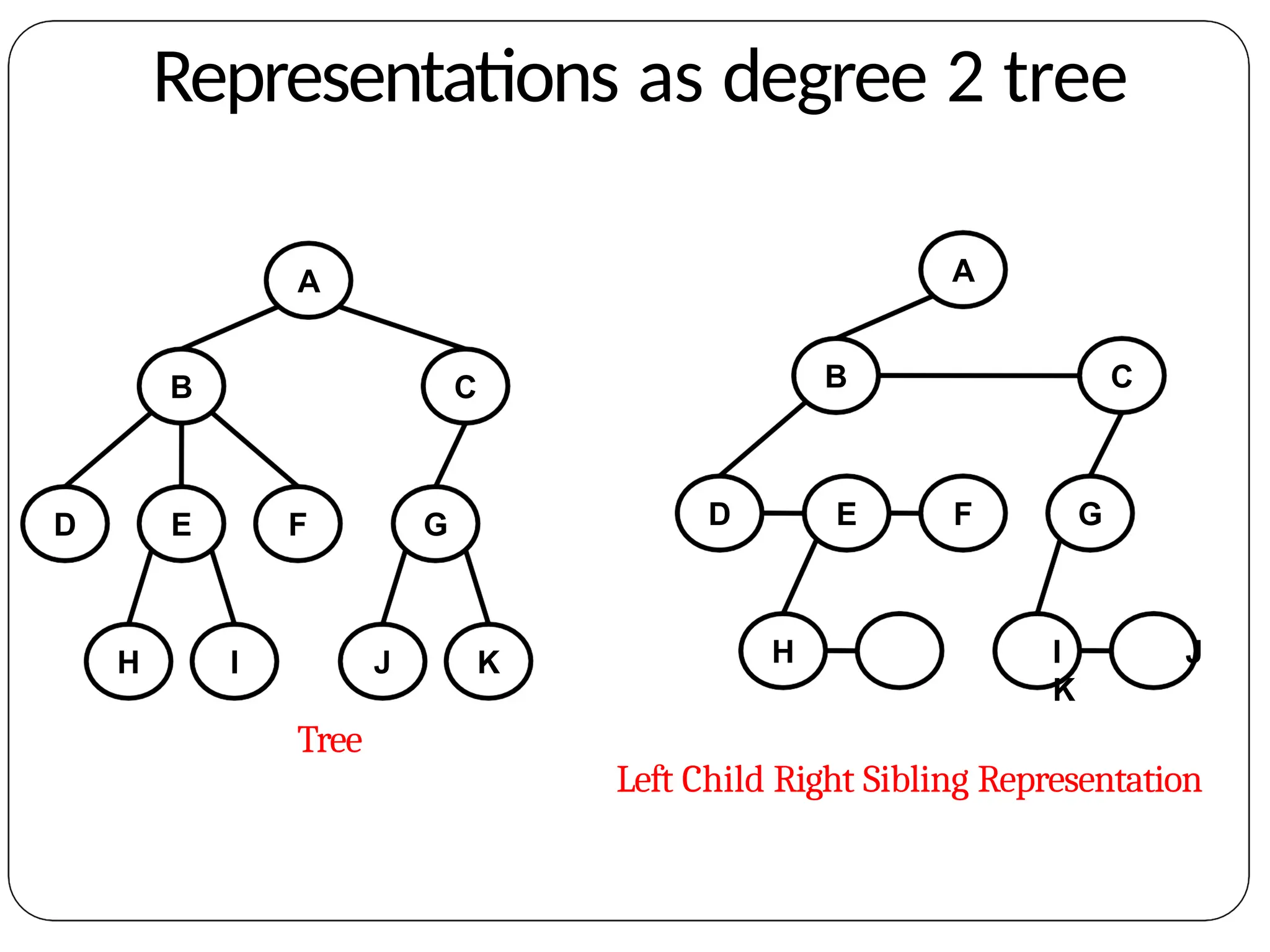
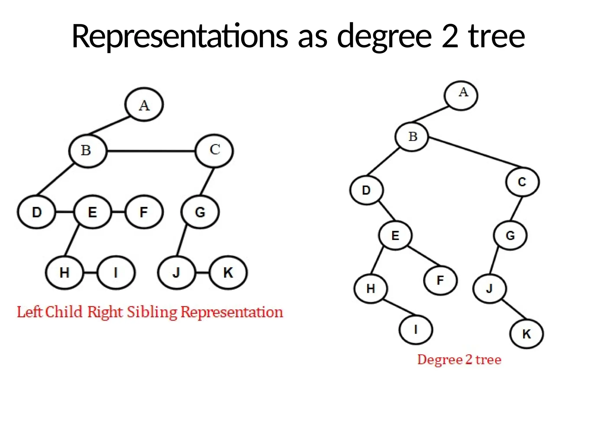
Representations as degree2 tree
Also known as Left child-Right child Tree/
Degree - Two Tree/ Binary Tree
Simply rotate the right sibling pointers in the
Left- child Right-sibling tree clockwise by 45 degrees
32.
Representations as degree2 tree
A
B C
D E F G
A
B C
D E F G
H I J K
Tree
H I J
K
Left Child Right Sibling Representation
Tree - Applications
Storing naturally hierarchical data: Trees are used to
store the data in the hierarchical structure. Example:
Directory structure of a file system
Organize data: It is used to organize data for efficient
insertion, deletion and searching.
Used in compression algorithms
Routing table: The tree data structure is also used to
store the data in routing tables in the routers.
To implement Heap data structure: It is used to
implement priority queues
35.
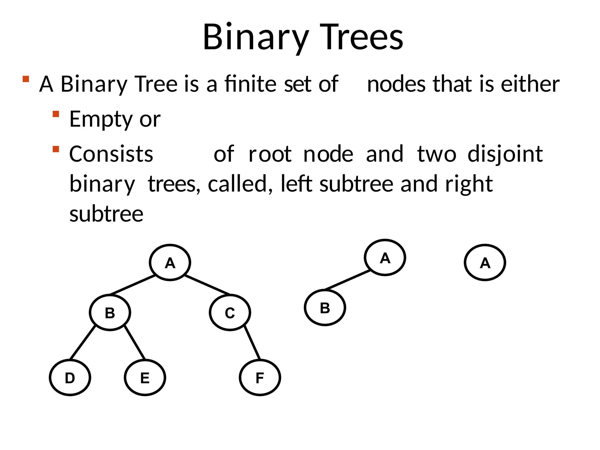
Binary Trees
ABinary Tree is a finite set of nodes that is either
Empty or
Consists of root node and two disjoint
binary trees, called, left subtree and right
subtree
A
B C
D E F
A
B
A
36.
Binary Trees
Anytree can be transformed into binary tree by left
child-right sibling representation
A tree can never be empty but binary tree can be
In binary tree a node can have atmost 2 children,
whereas in case of a tree, a node may have any
number of children
37.
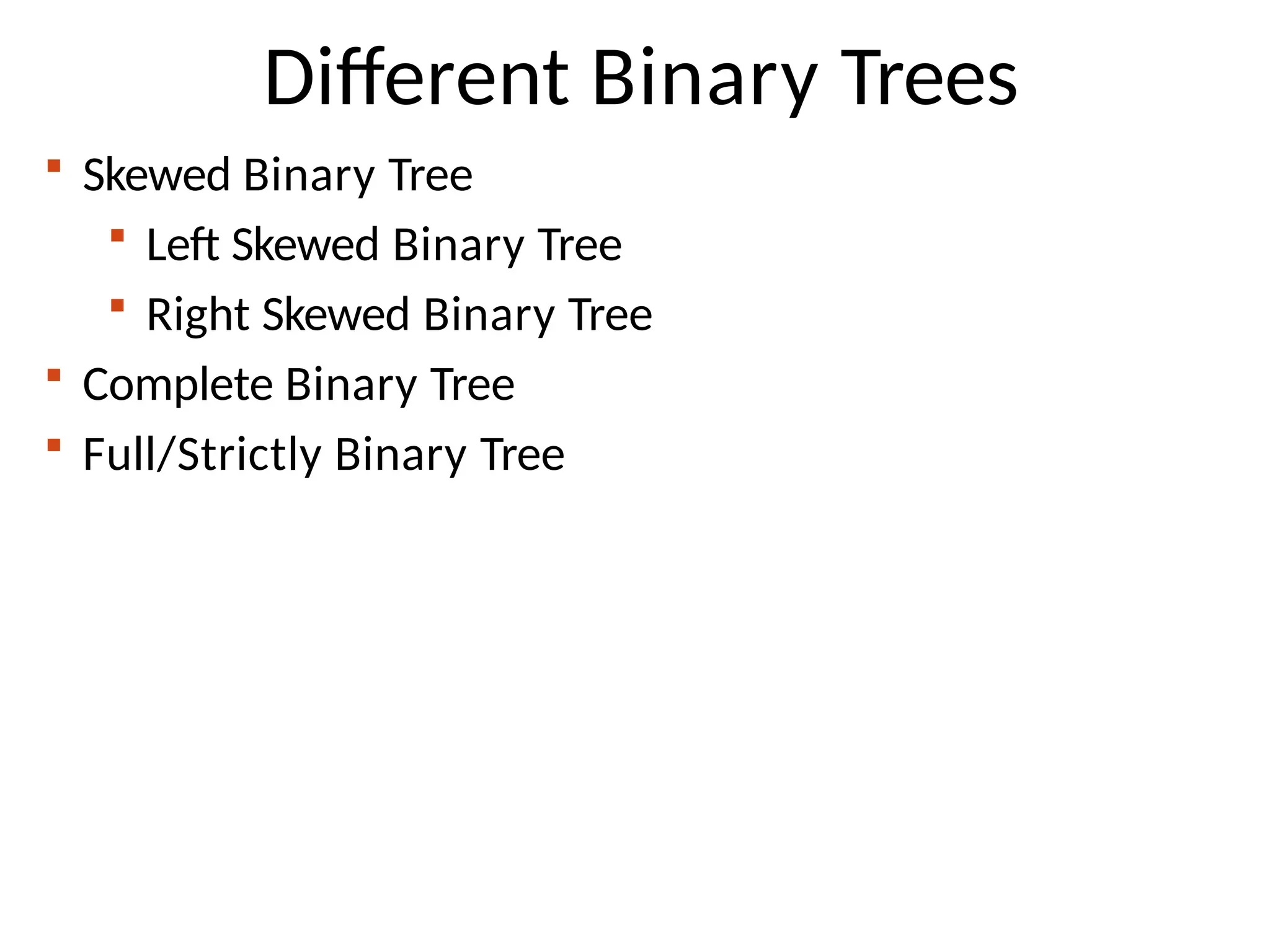
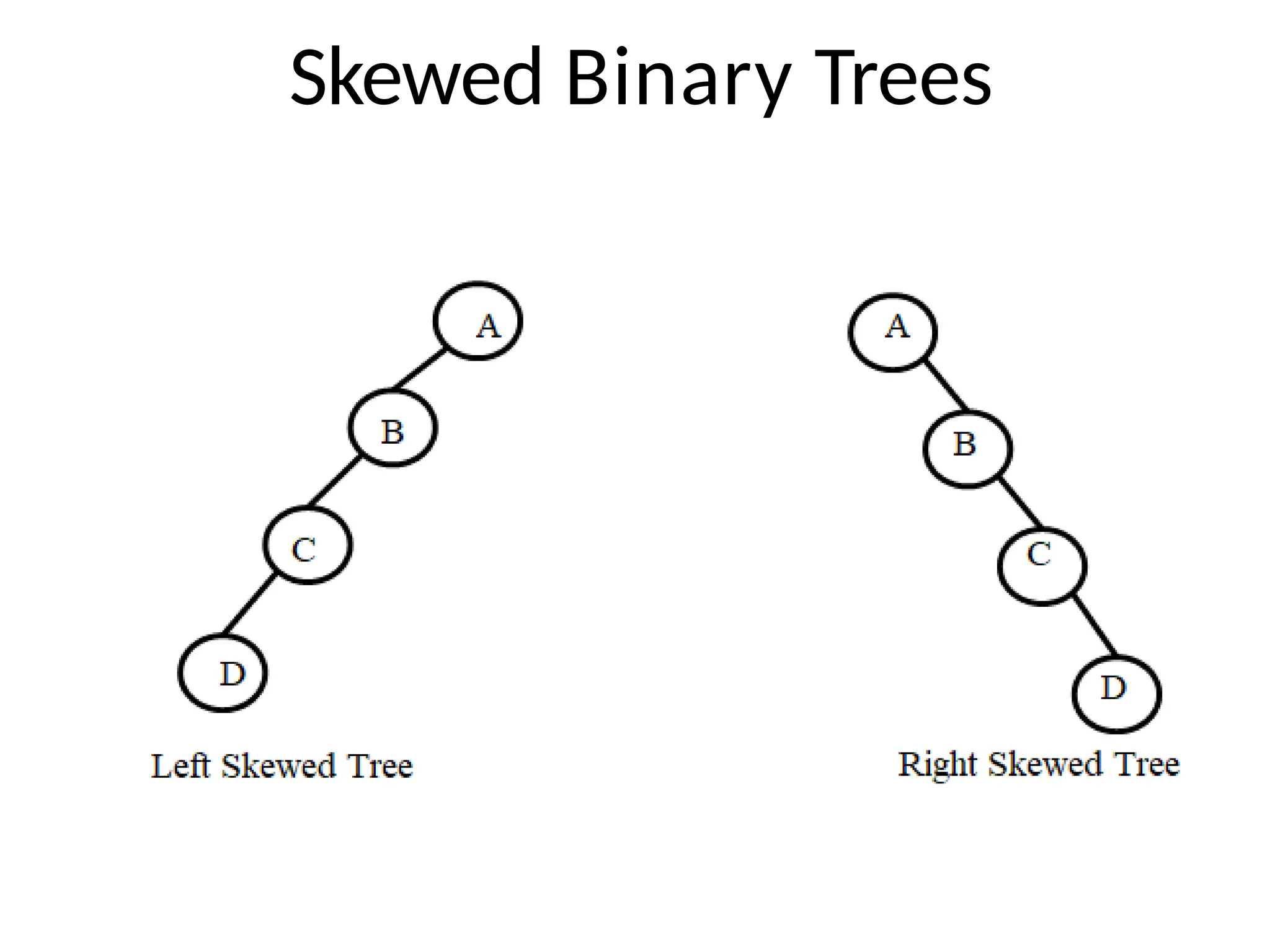
Different Binary Trees
Skewed Binary Tree
Left Skewed Binary Tree
Right Skewed Binary Tree
Complete Binary Tree
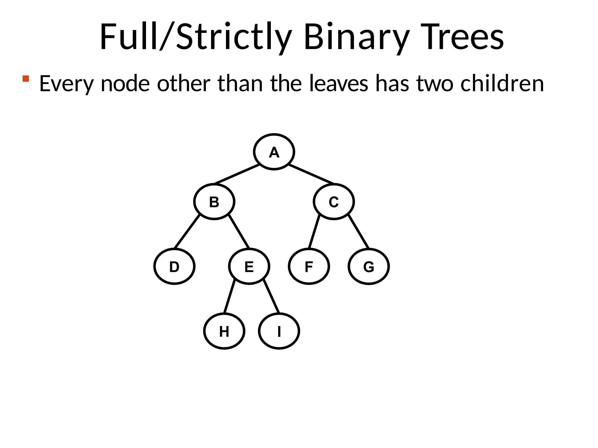
Full/Strictly Binary Tree
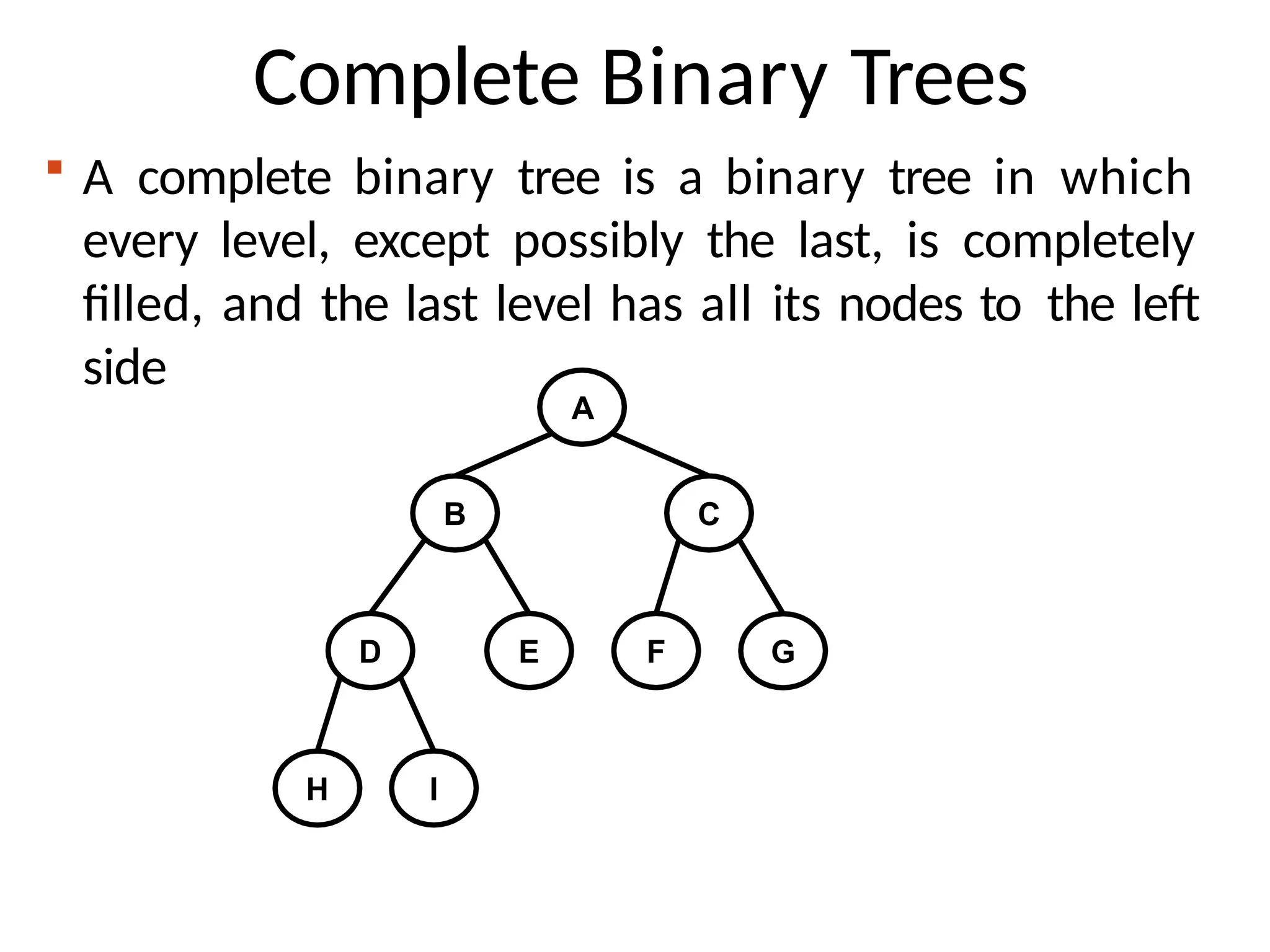
Complete Binary Trees
A complete binary tree is a binary tree in which
every level, except possibly the last, is completely
filled, and the last level has all its nodes to the left
side
A
B C
D E F
H I
G
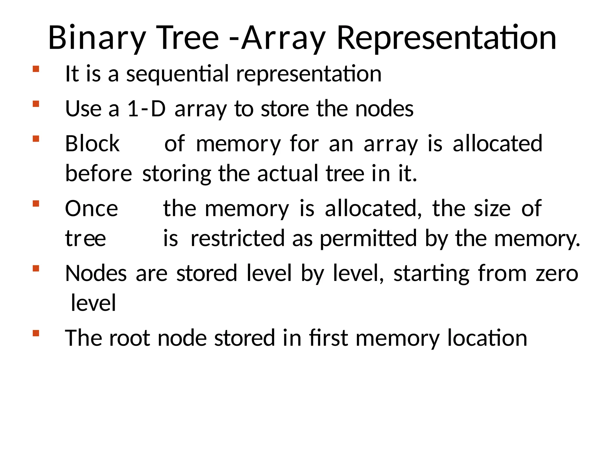
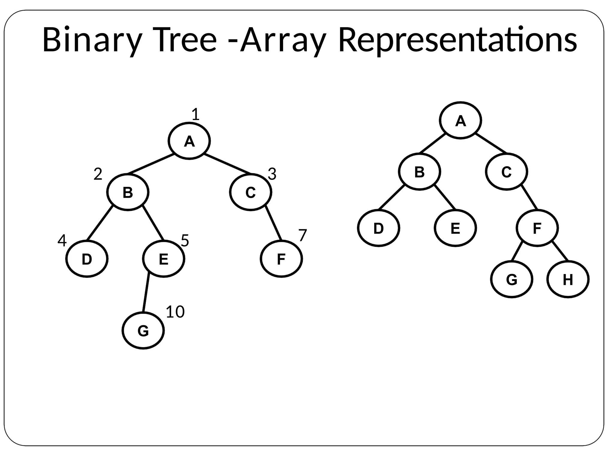
Binary Tree -ArrayRepresentation
It is a sequential representation
Use a 1-D array to store the nodes
Block of memory for an array is allocated
before storing the actual tree in it.
Once the memory is allocated, the size of
tree is restricted as permitted by the memory.
Nodes are stored level by level, starting from zero
level
The root node stored in first memory location
43.
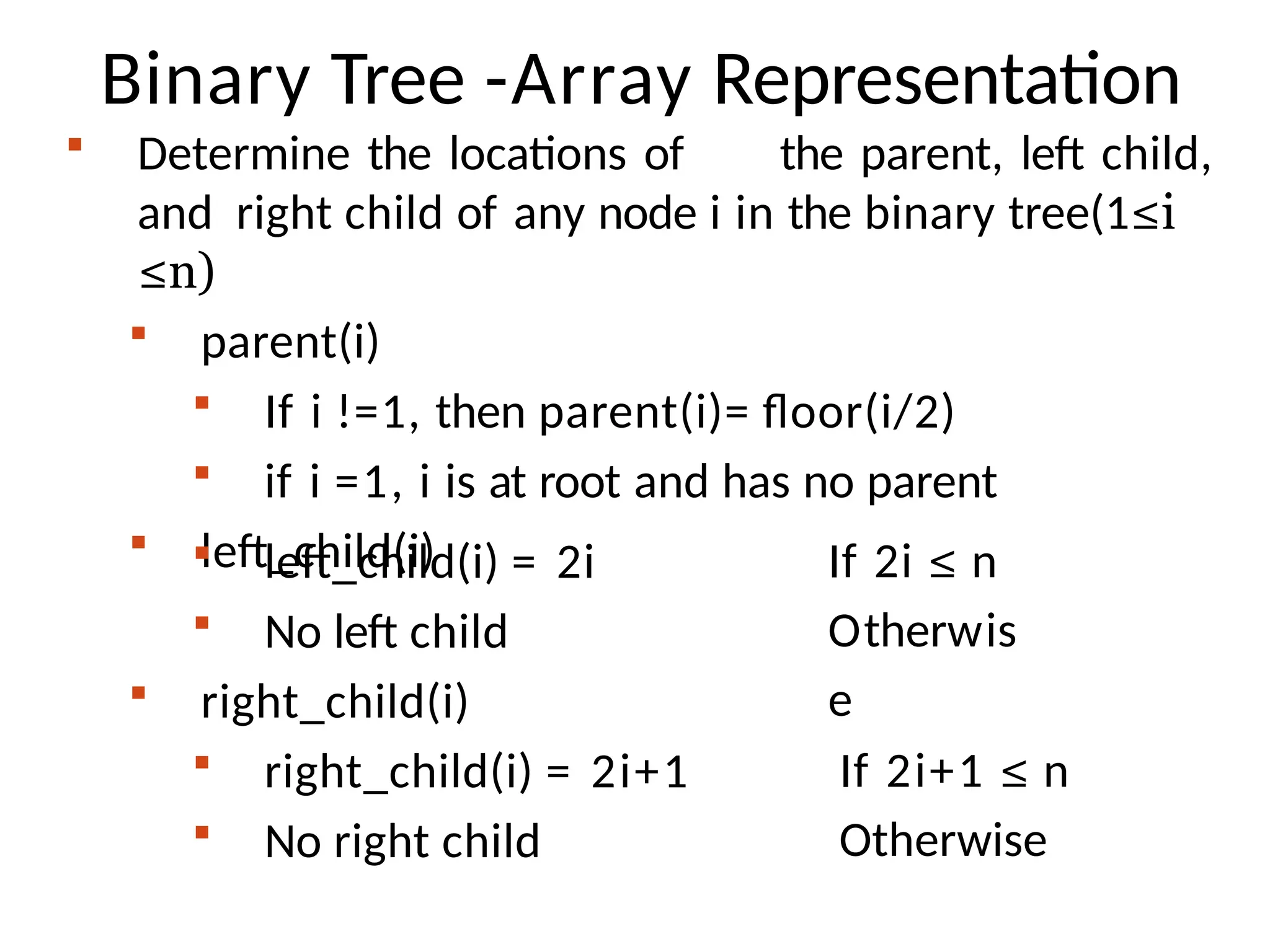
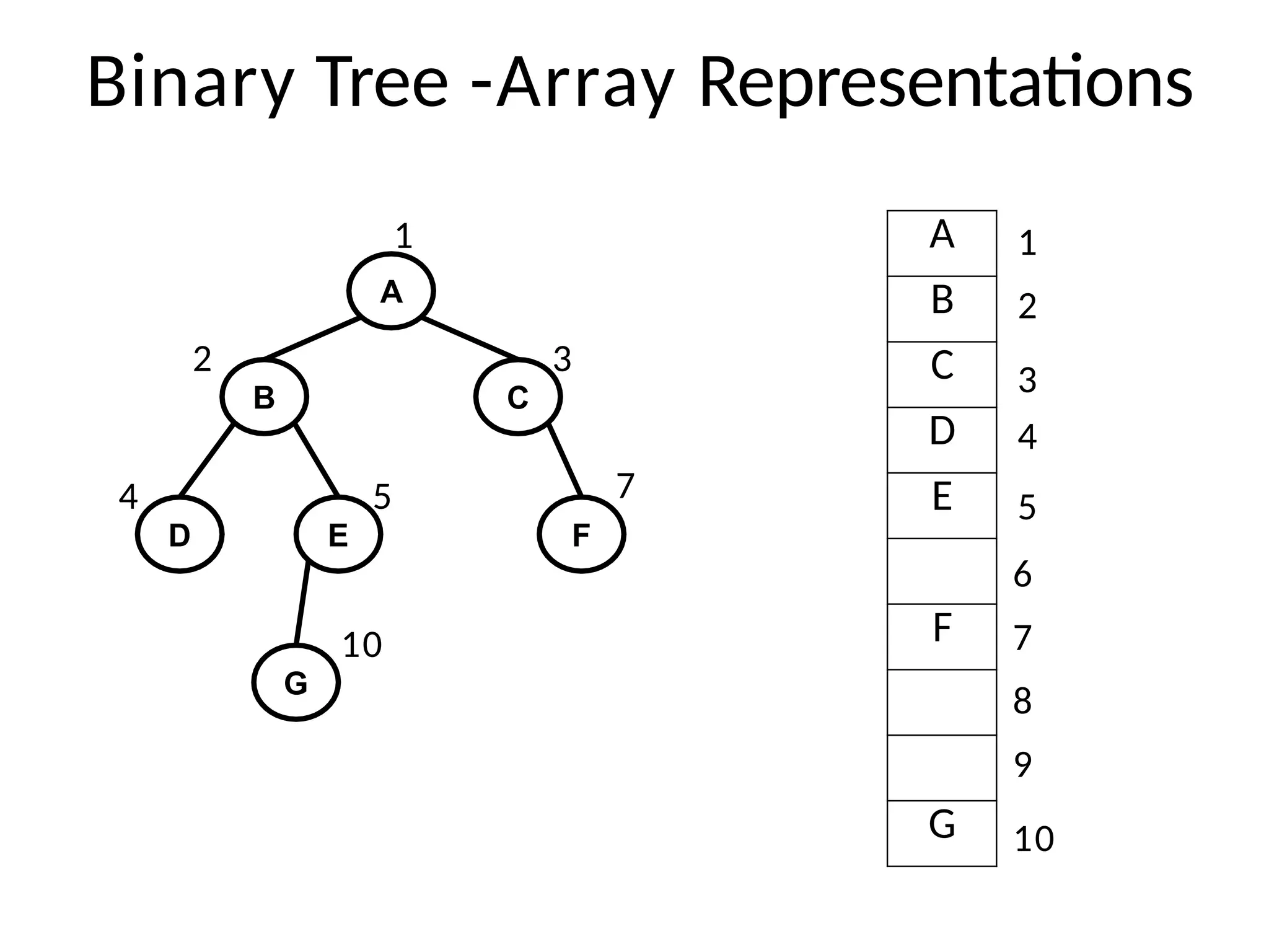
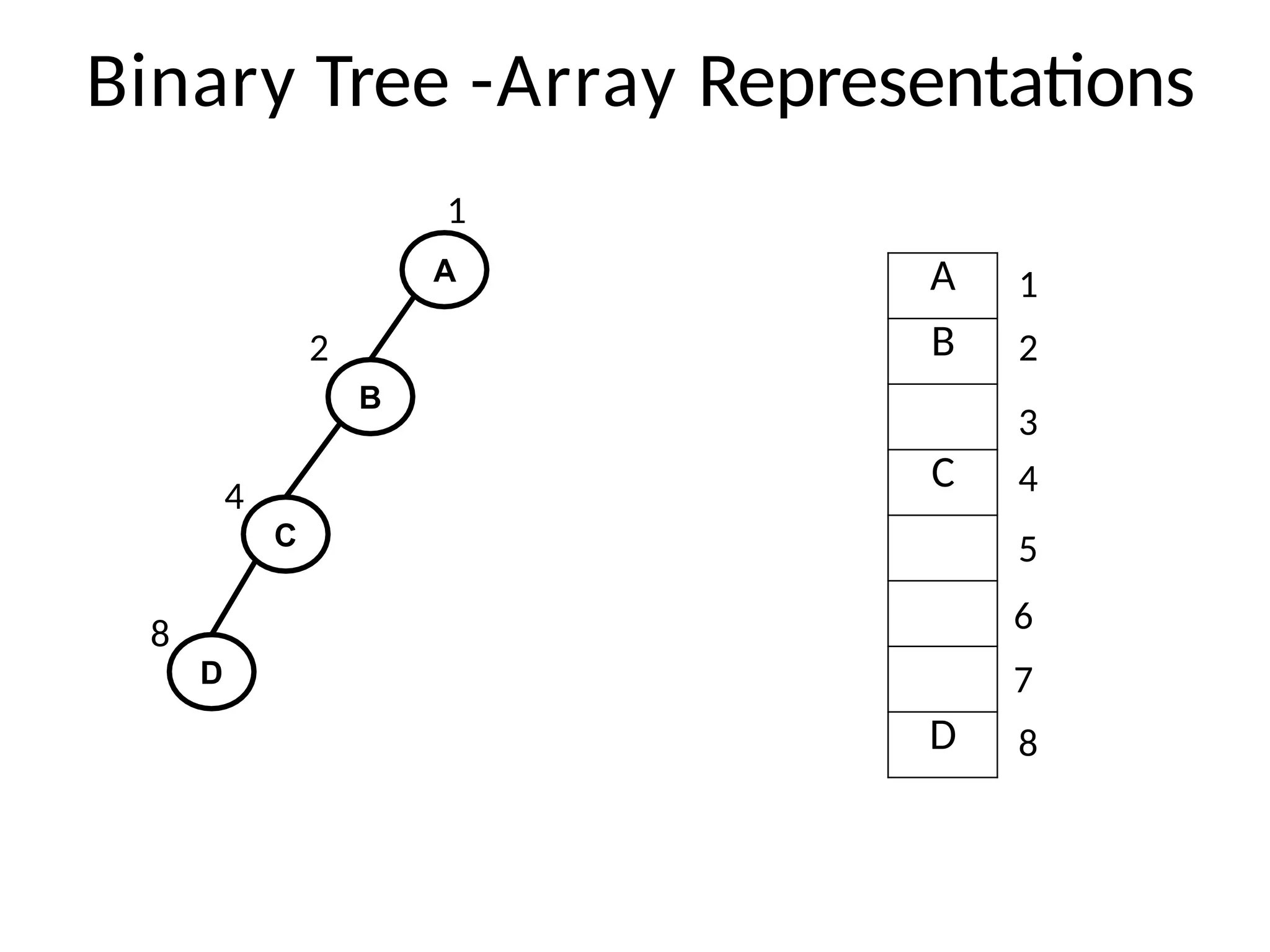
Binary Tree -ArrayRepresentation
Determine the locations of the parent, left child,
and right child of any node i in the binary tree(1≤i
≤n)
parent(i)
If i !=1, then parent(i)= floor(i/2)
if i =1, i is at root and has no parent
left_child(i)
left_child(i) = 2i
No left child
If 2i ≤ n
Otherwis
e
right_child(i)
right_child(i) = 2i+1
No right child
If 2i+1 ≤ n
Otherwise
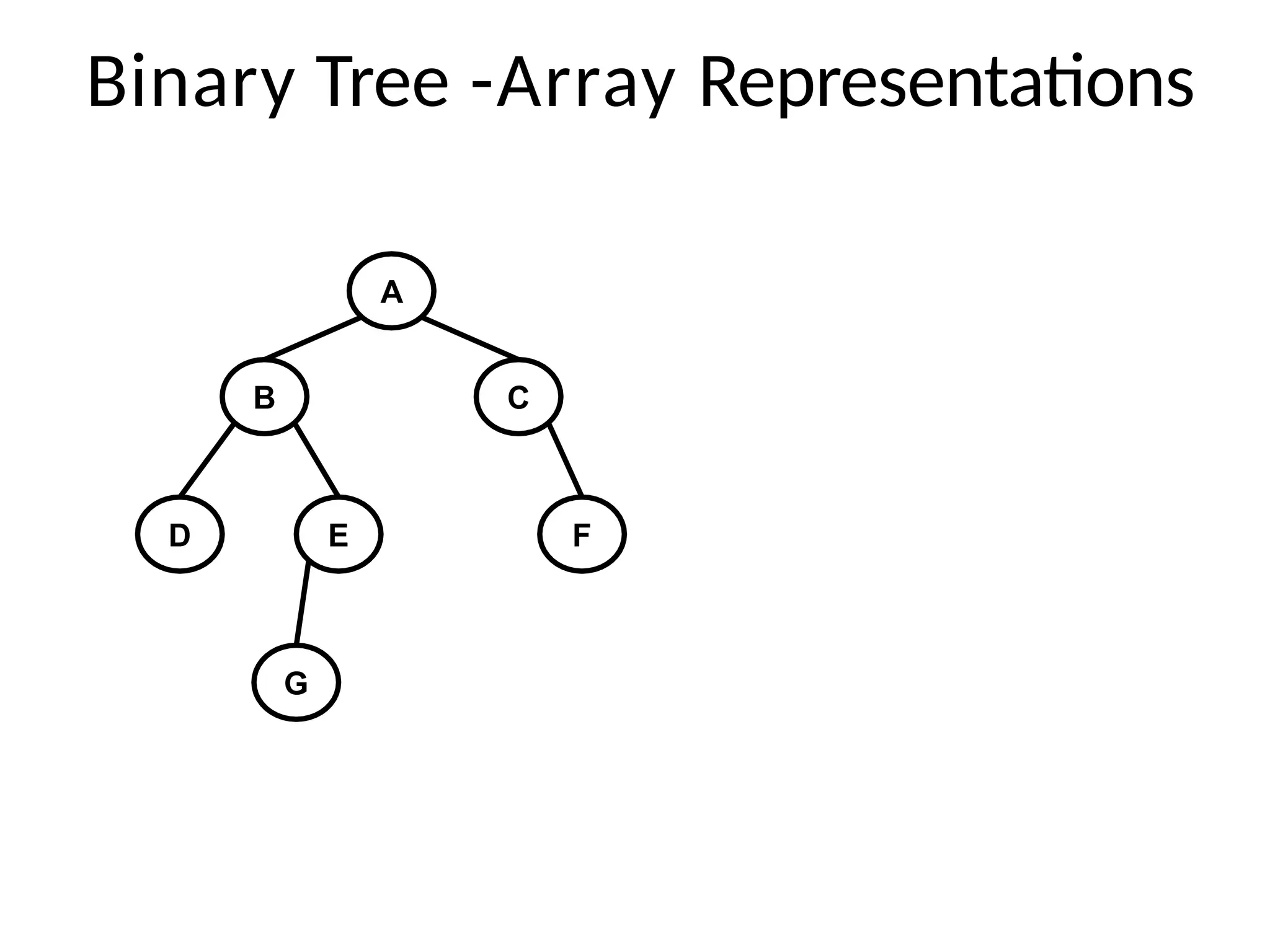
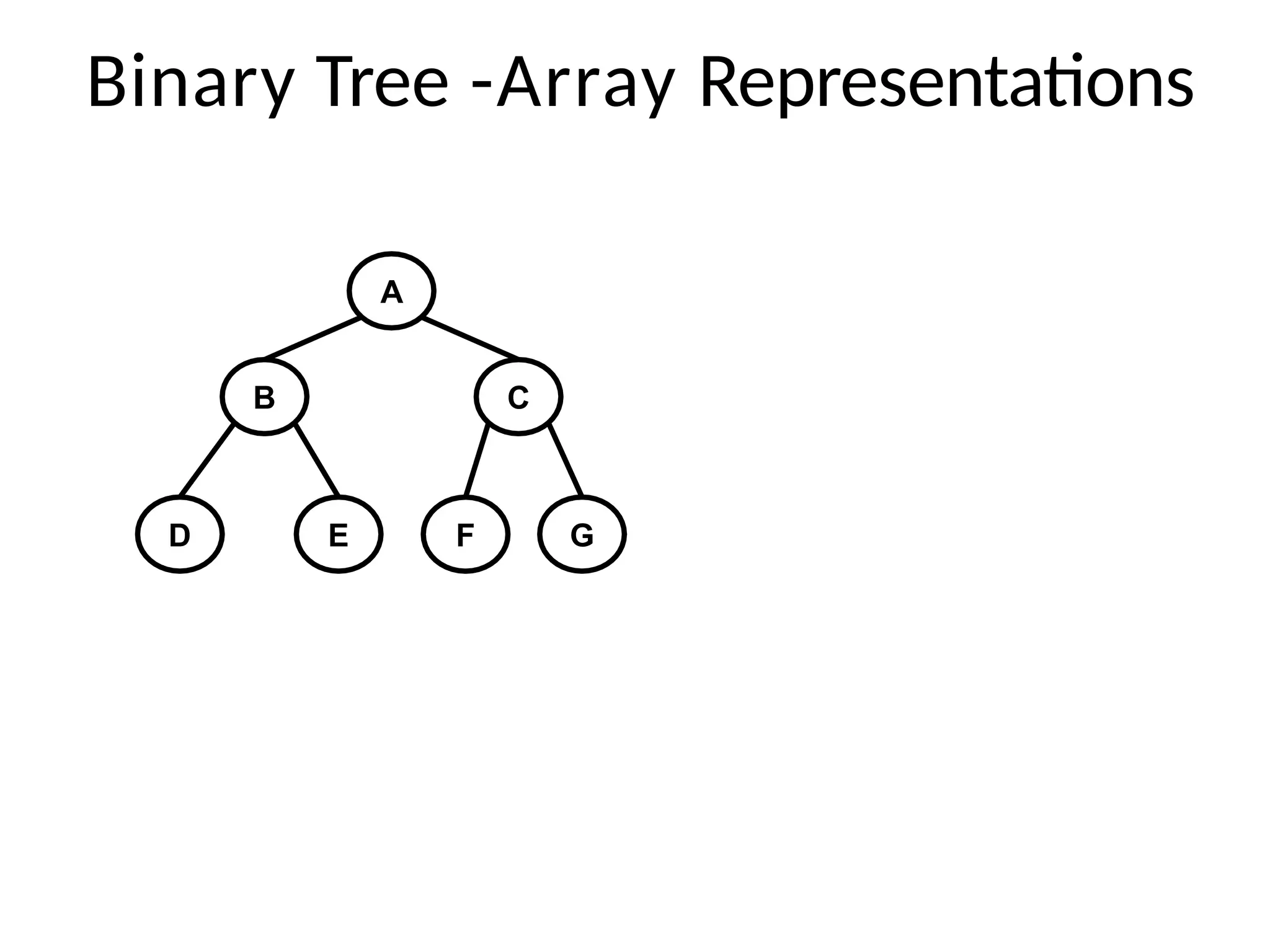
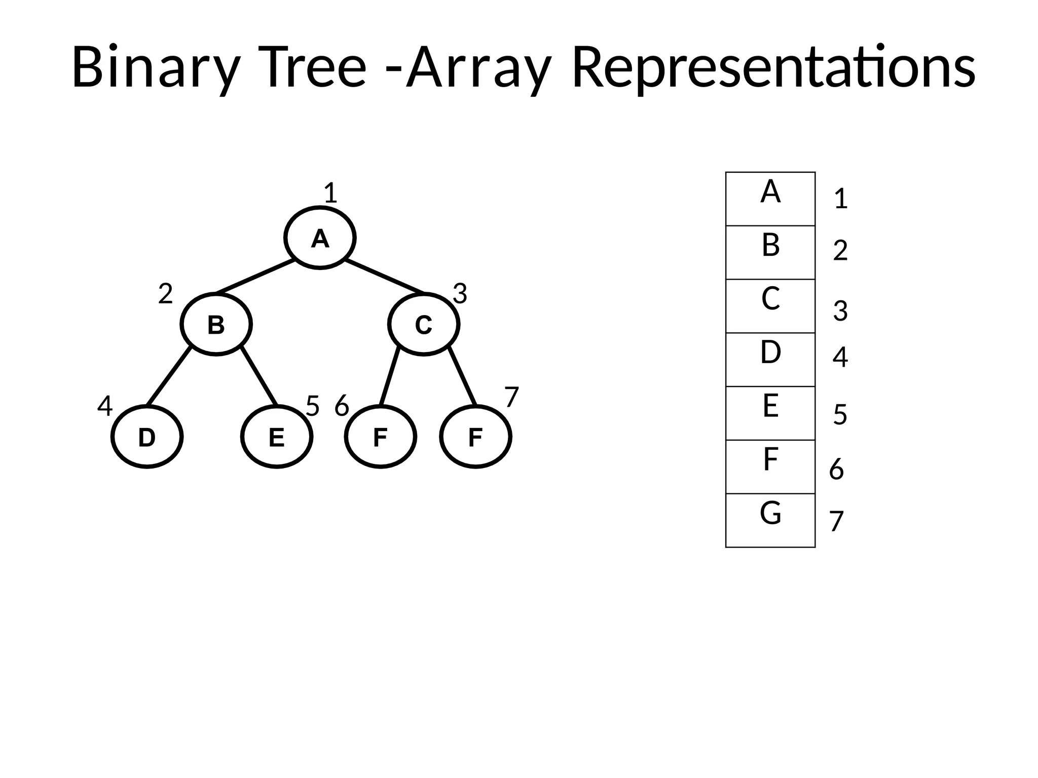
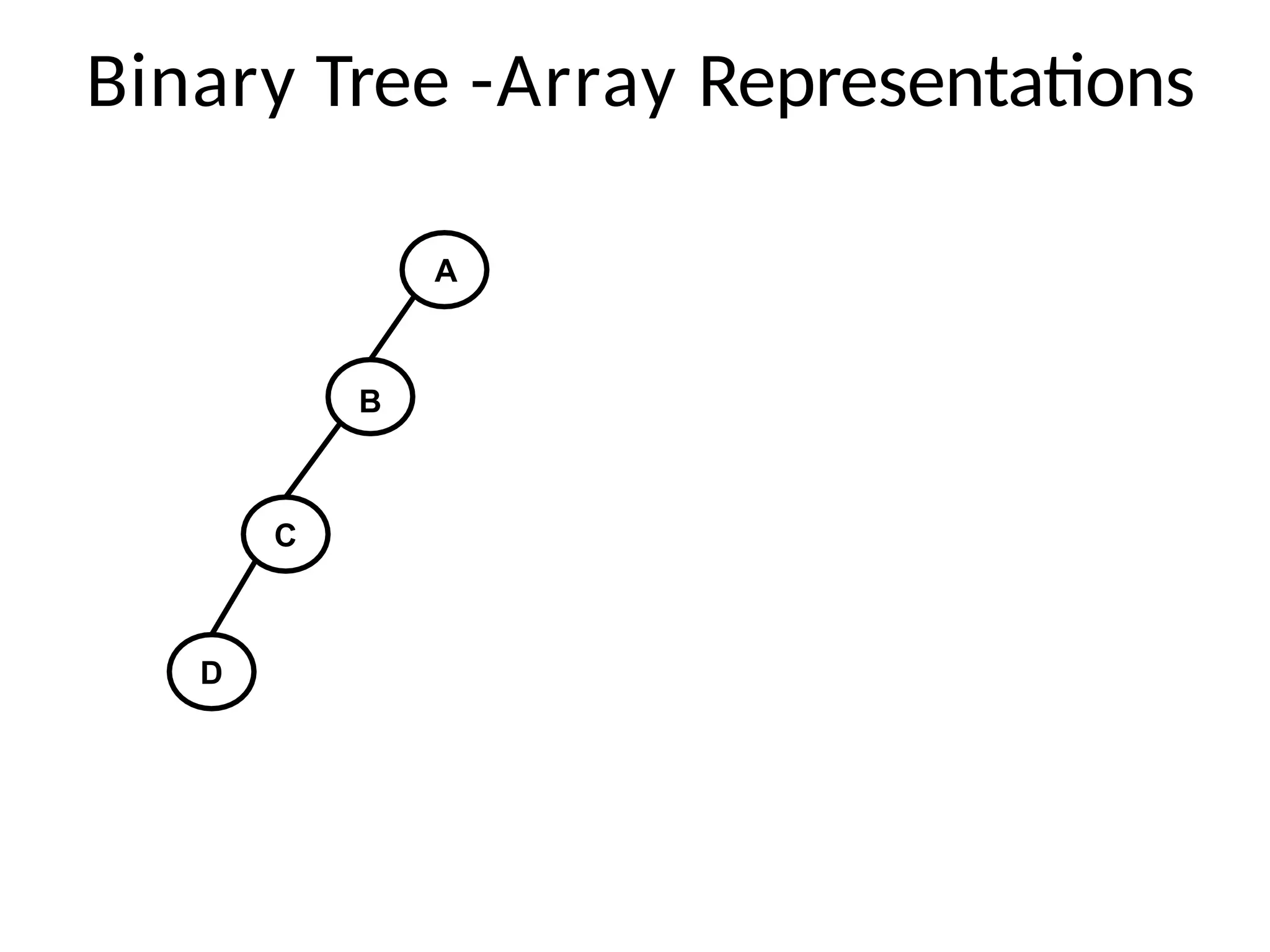
Binary Tree -ArrayRepresentations
A
B
C
D
A
B
C
D
1
2
3
4
5
6
7
8
1
2
4
8
51.
Binary Tree -ArrayRepresentations
Advantages
Any node can be accessed from any other node by
calculating the index.
Data are stored without any pointer
Programming languages, where dynamic memory
allocation is not possible(like BASIC, FROTRAN),
array representation is only possible
Good for Complete Binary tree.
Searching is fast
52.
Binary Tree -ArrayRepresentations
Disadvantages
Good for Complete Binary tree. If it is not a
complete binary tree then, a lot of memory is
wasted
Dynamic memory allocation is not possible
53.
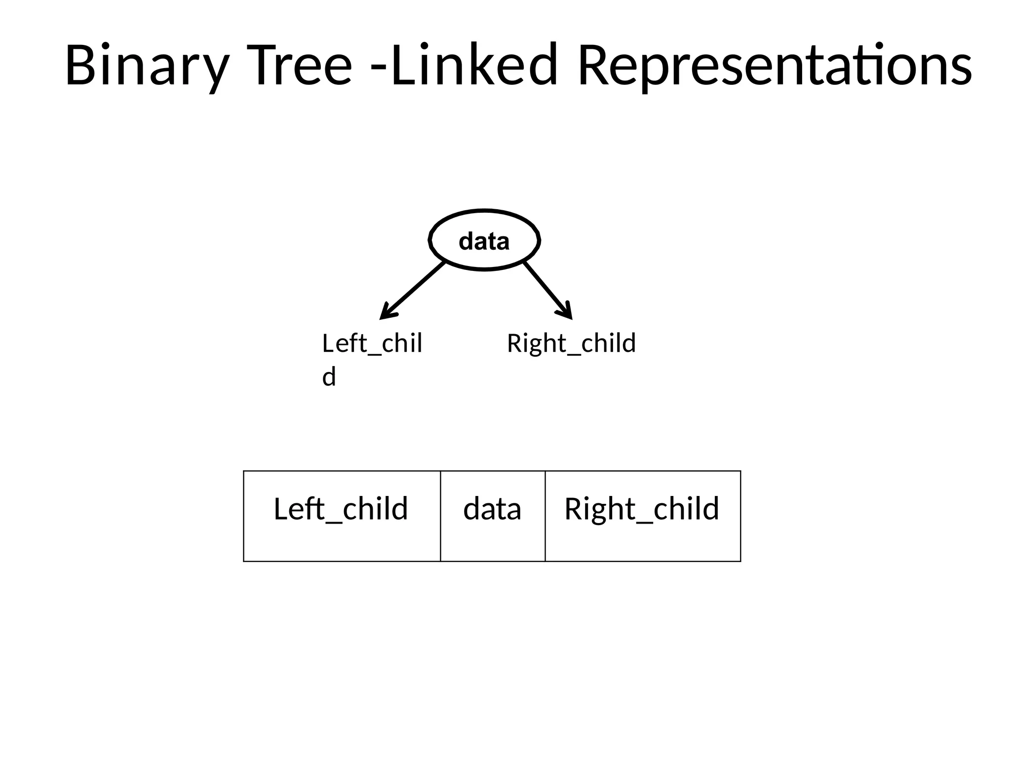
Binary Tree -LinkedRepresentations
data
Left_chil
d
Right_child
Left_child data Right_child
54.
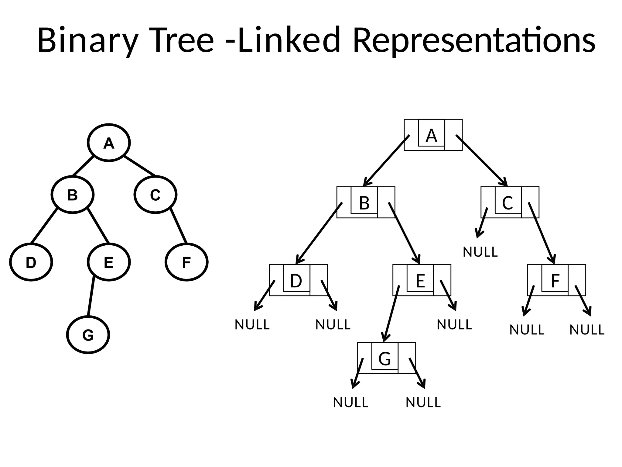
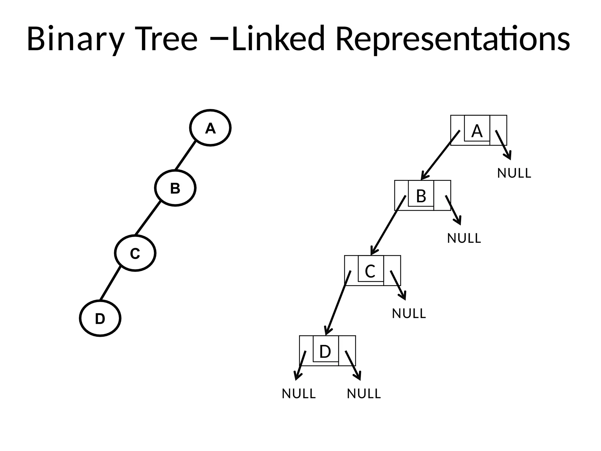
Binary Tree -LinkedRepresentations
A
B C
D E F
G
A
B C
F
D E
G
NULL NULL
NULL NULL
NULL
NULL NULL NULL
Binary Tree -LinkedRepresentations
Advantages
Dynamic memory allocation is possible
57.
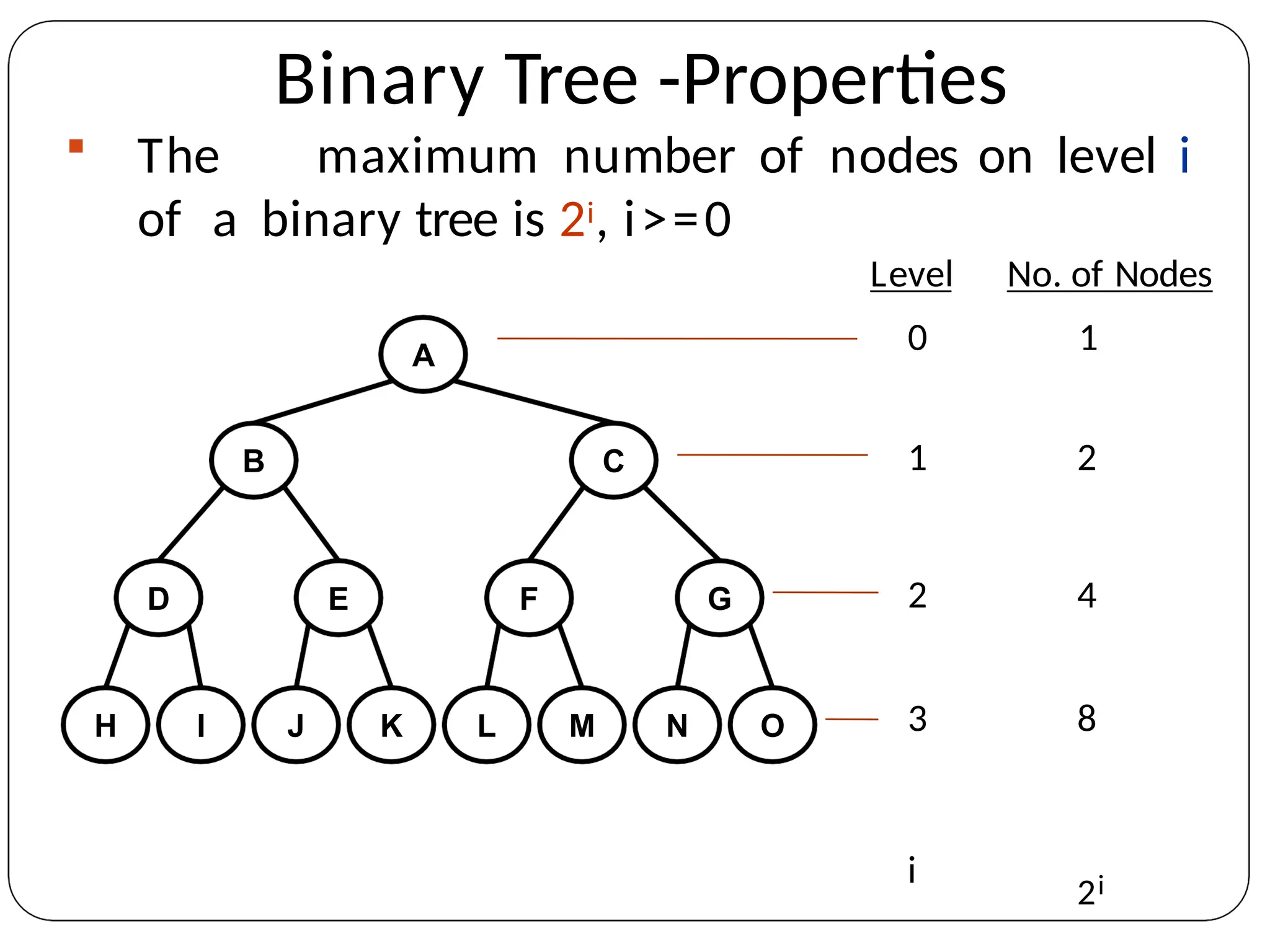
Binary Tree -Properties
The maximum number of nodes on level i
of a binary tree is 2i, i>=0
A
B C
D E G
F
H I J K L M N O
Level
0
No. of Nodes
1
1 2
2 4
3 8
i
2i
58.
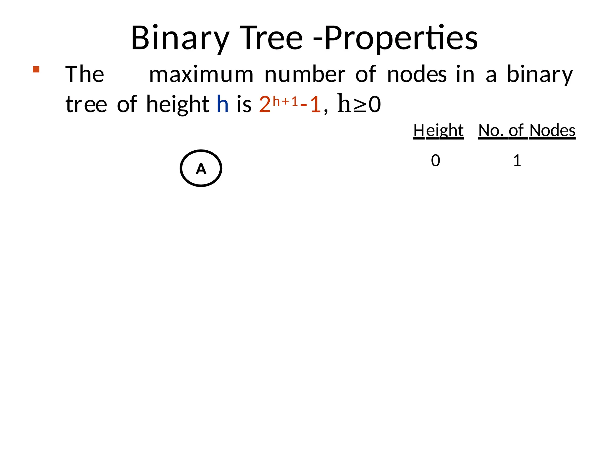
Binary Tree -Properties
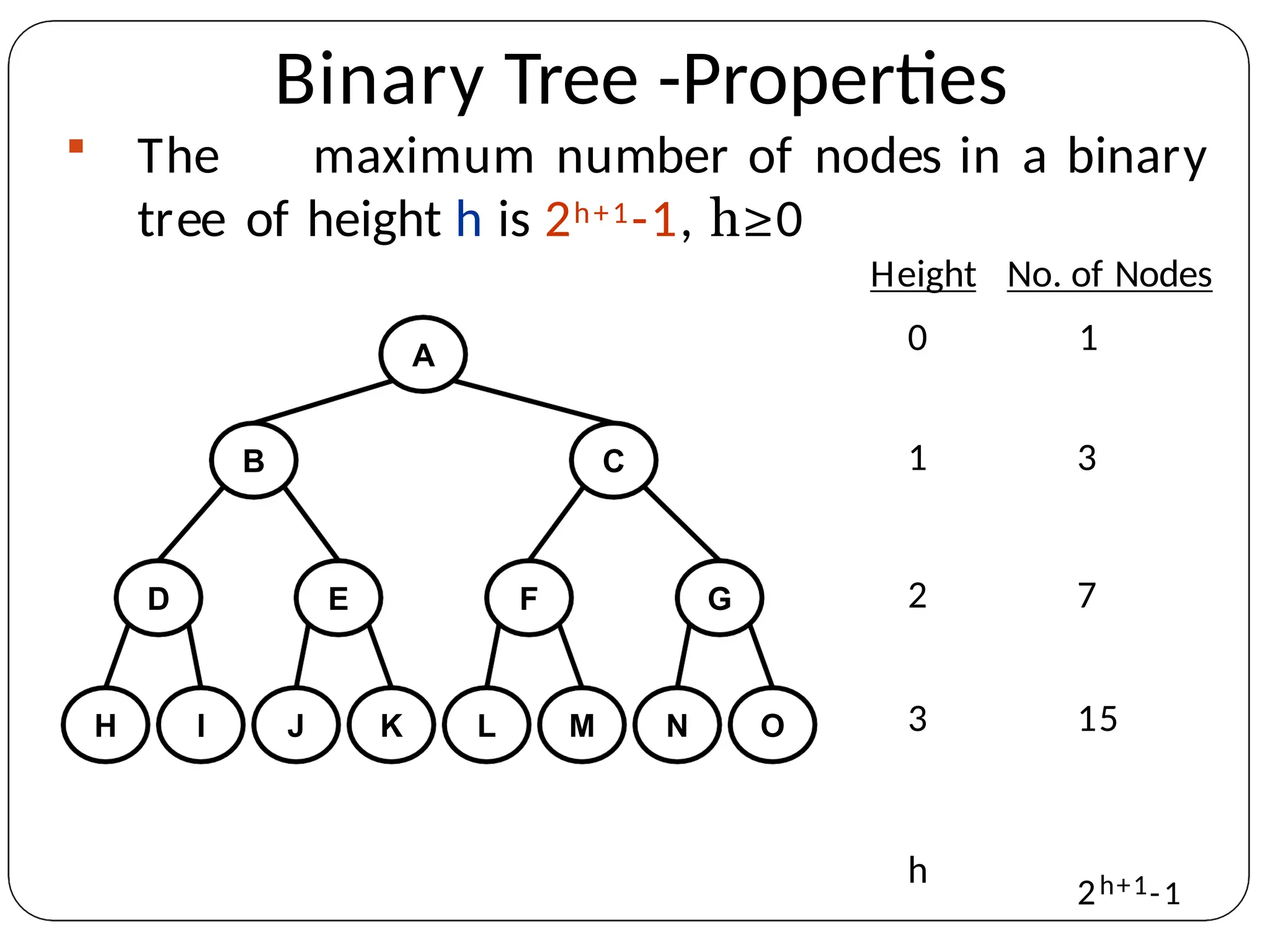
The maximum number of nodes in a binary
tree of height h is 2h+1-1, h≥0
A
Height
0
No. of Nodes
1
59.
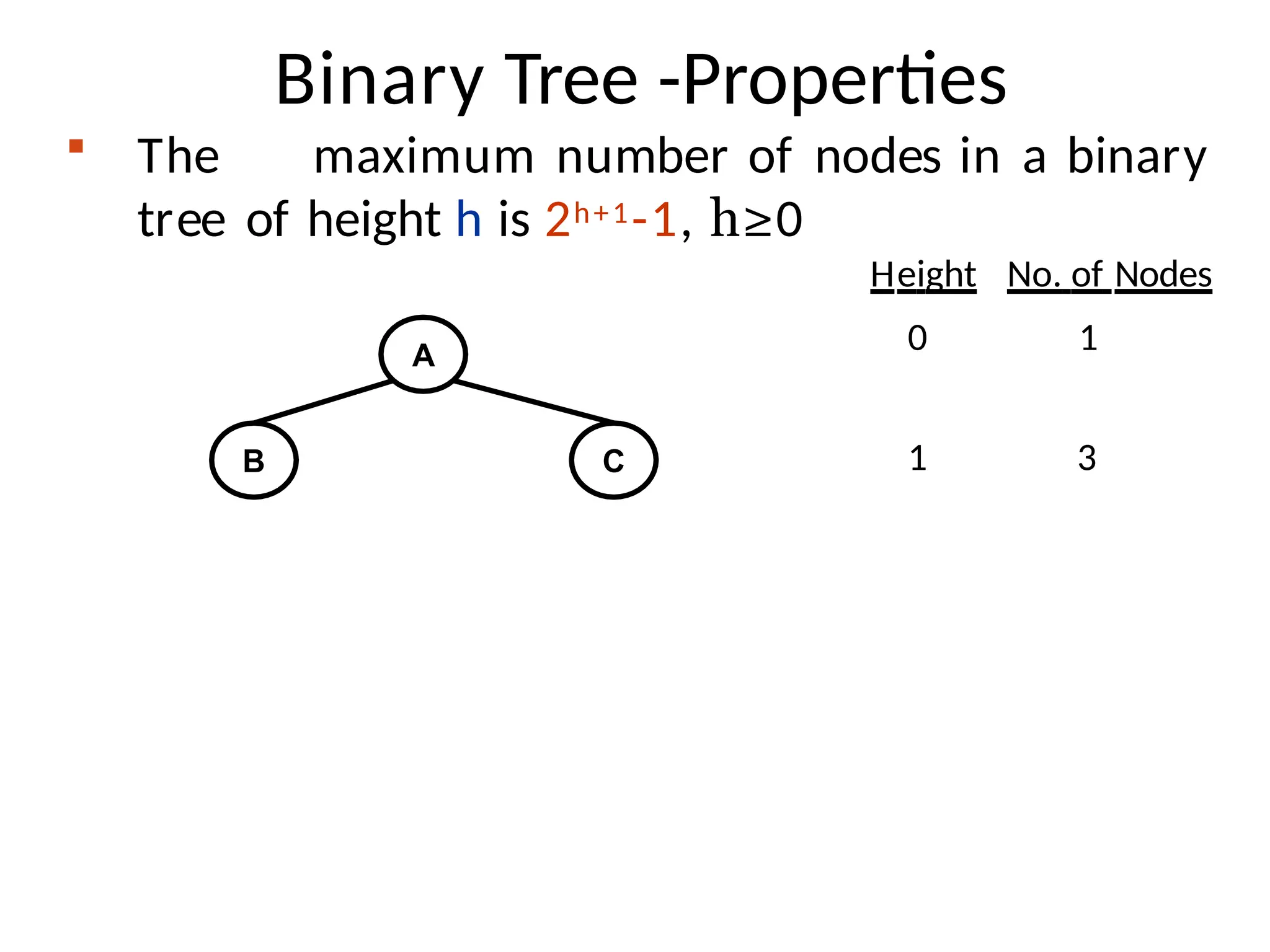
Binary Tree -Properties
The maximum number of nodes in a binary
tree of height h is 2h+1-1, h≥0
A
B C
Height
0
No. of Nodes
1
1 3
60.
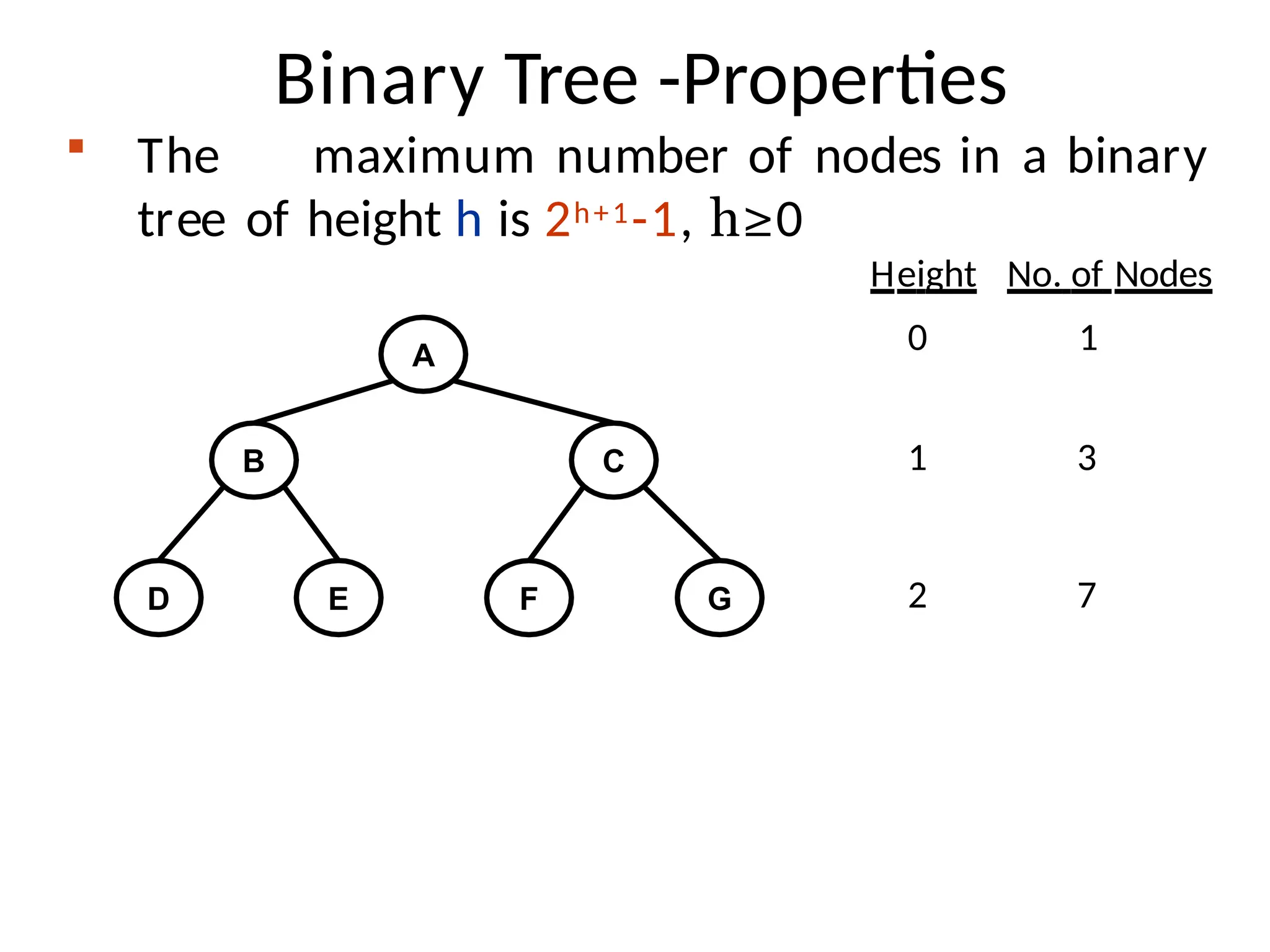
Binary Tree -Properties
The maximum number of nodes in a binary
tree of height h is 2h+1-1, h≥0
A
B C
D E G
F
Height
0
No. of Nodes
1
1 3
2 7
61.
Binary Tree -Properties
The maximum number of nodes in a binary
tree of height h is 2h+1-1, h≥0
A
B C
D E G
F
H I J K L M N O
Height
0
No. of Nodes
1
1 3
2 7
3 15
62.
Binary Tree -Properties
The maximum number of nodes in a binary
tree of height h is 2h+1-1, h≥0
A
B C
D E G
F
H I J K L M N O
Height
0
No. of Nodes
1
1 3
2 7
3 15
h
2h+1-1
63.
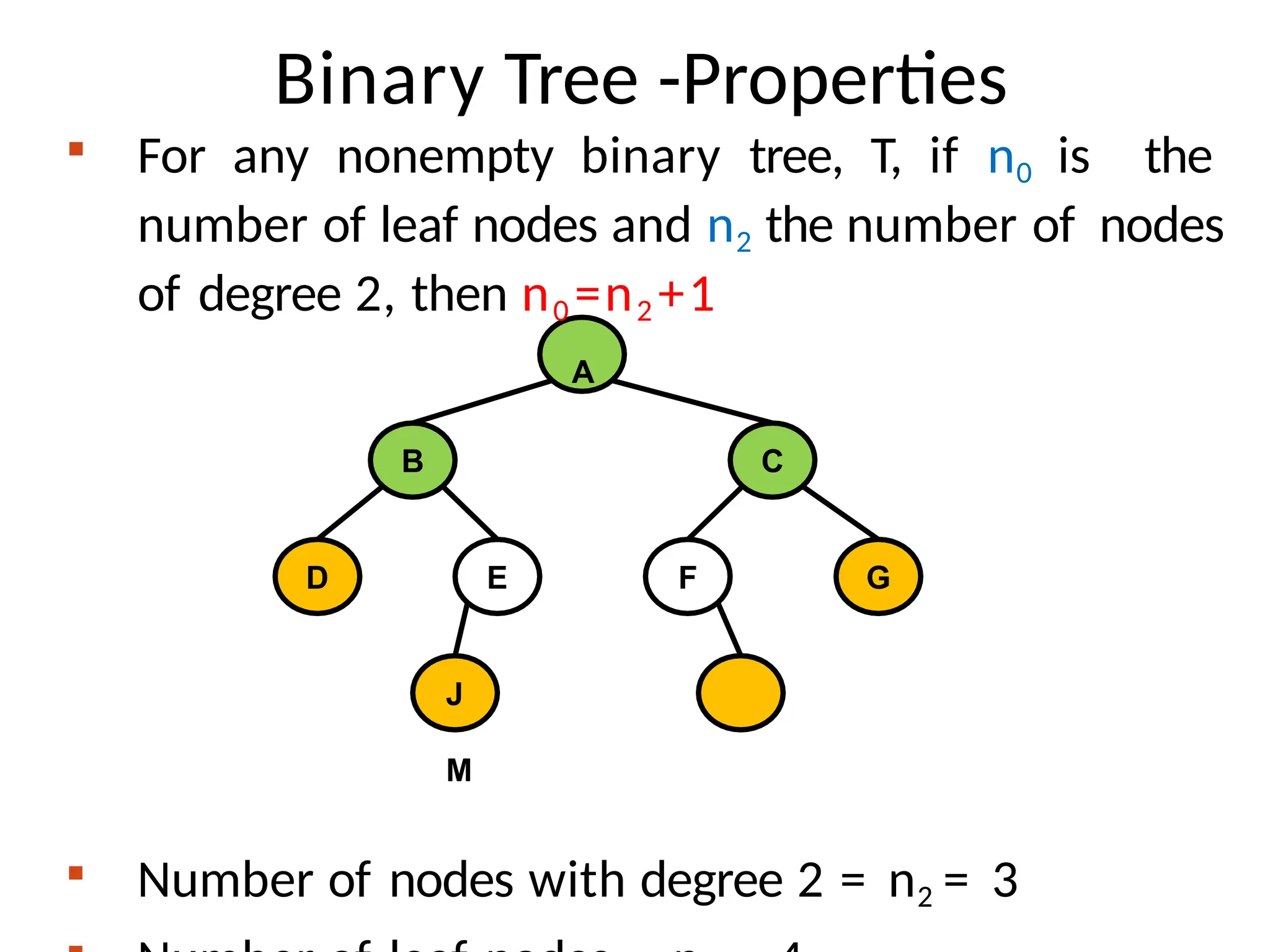
Binary Tree -Properties
For any nonempty binary tree, T, if n0 is the
number of leaf nodes and n2 the number of nodes
of degree 2, then n0 =n2 +1
A
B C
D E G
F
J
M
Number of nodes with degree 2 = n2 = 3
64.
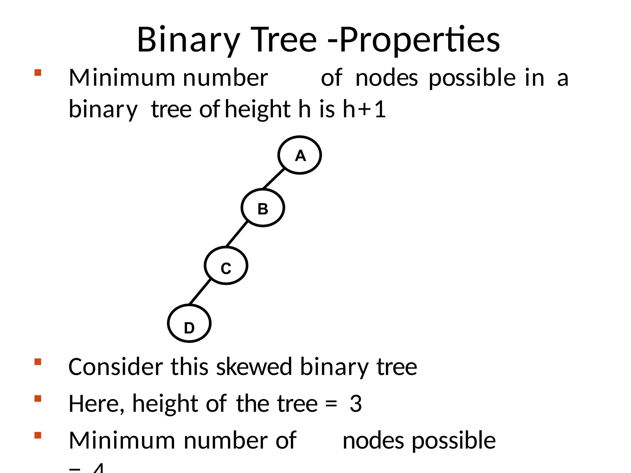
Binary Tree -Properties
Minimum number of nodes possible in a
binary tree ofheight h is h+1
Consider this skewed binary tree
Here, height of the tree = 3
Minimum number of nodes possible
A
B
C
D
65.
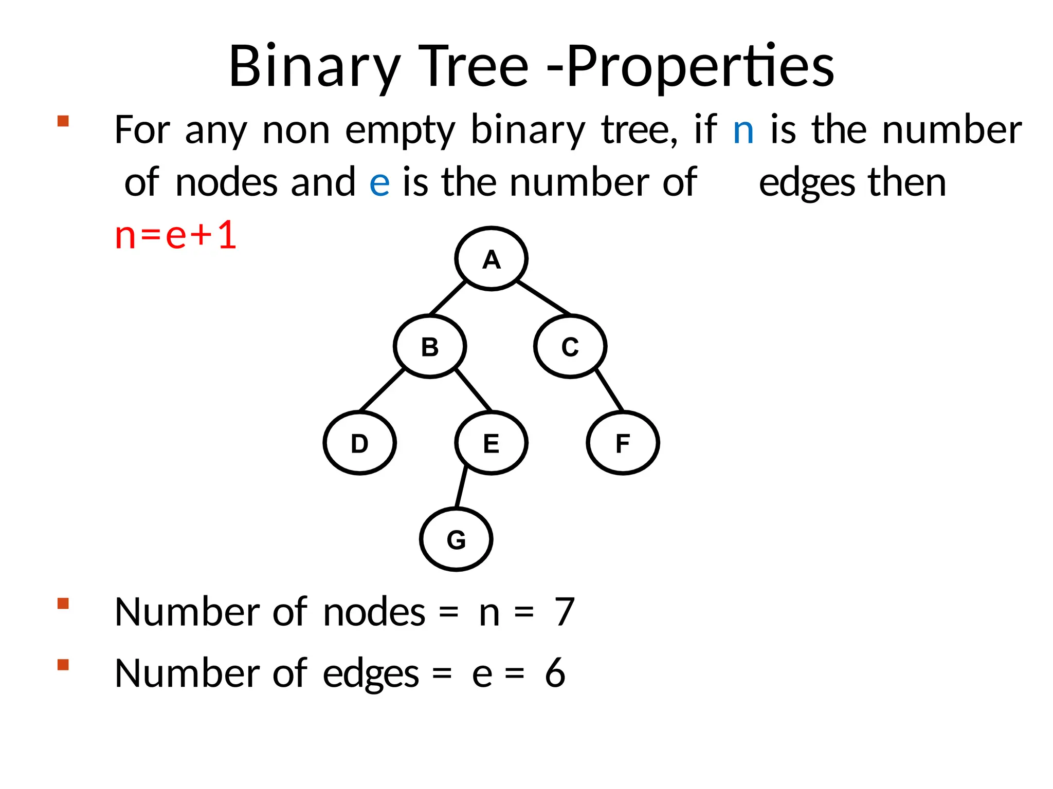
Binary Tree -Properties
For any non empty binary tree, if n is the number
of nodes and e is the number of edges then
n=e+1
Number of nodes = n = 7
Number of edges = e = 6
A
B C
D E F
G
66.
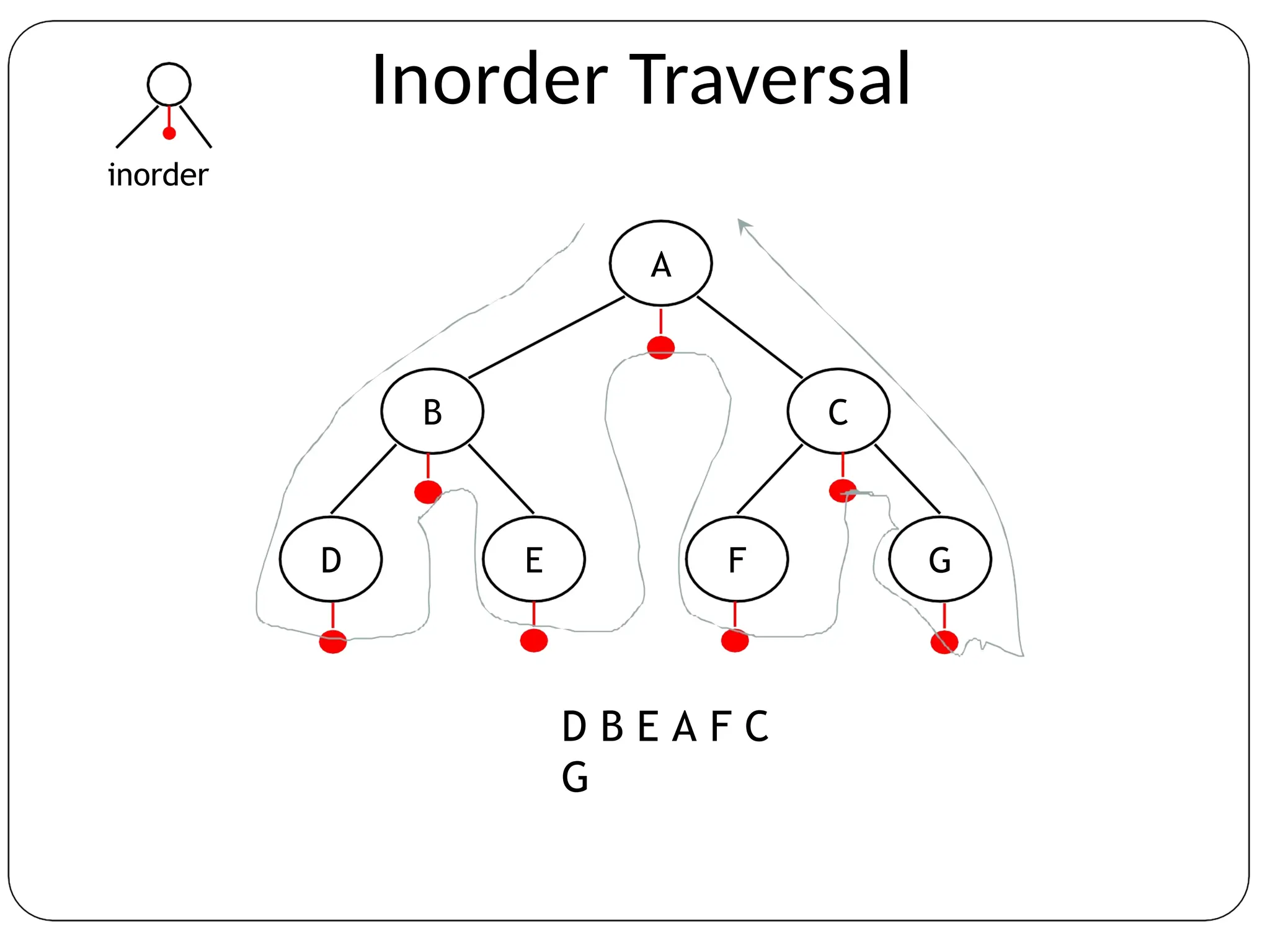
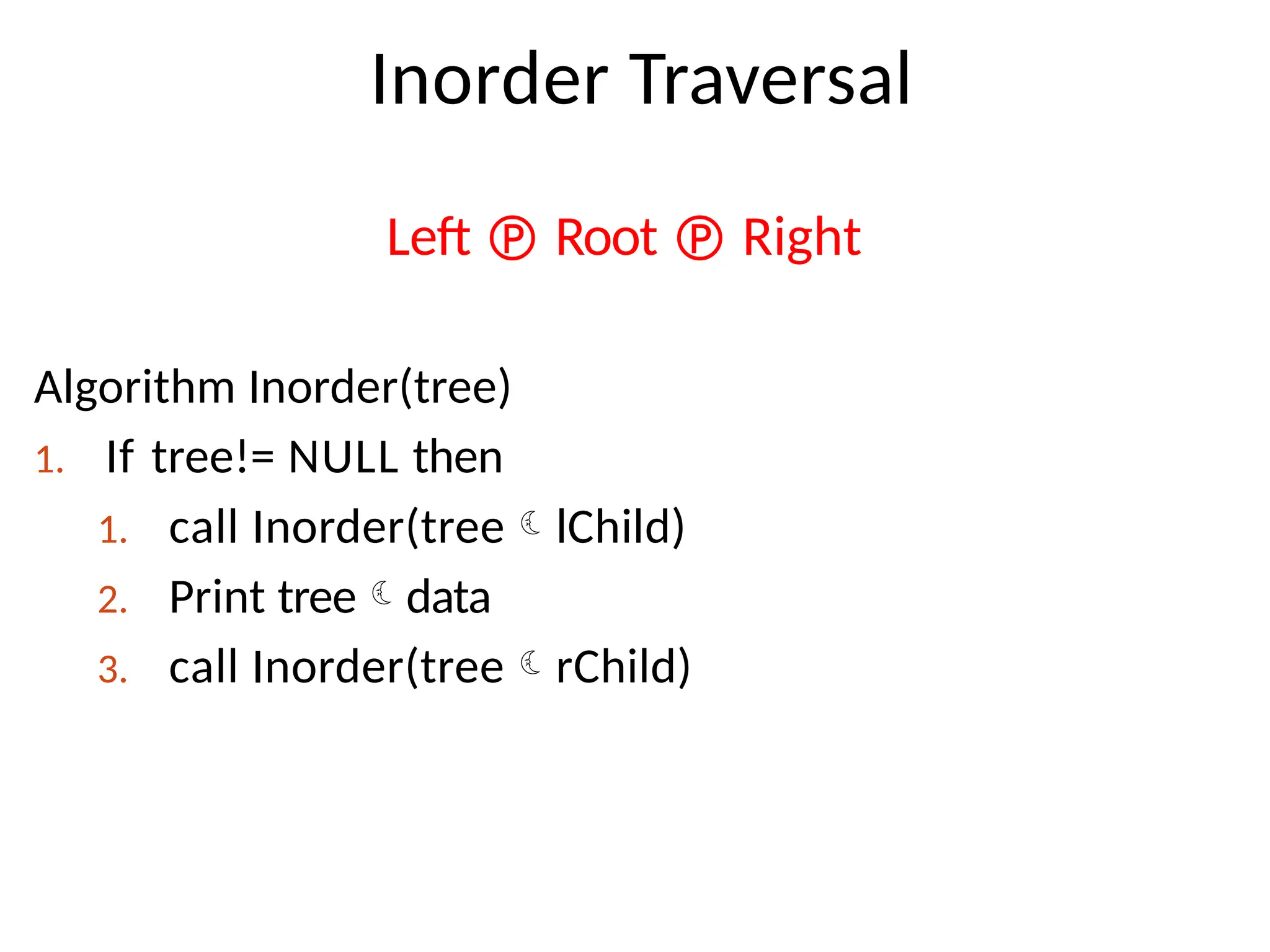
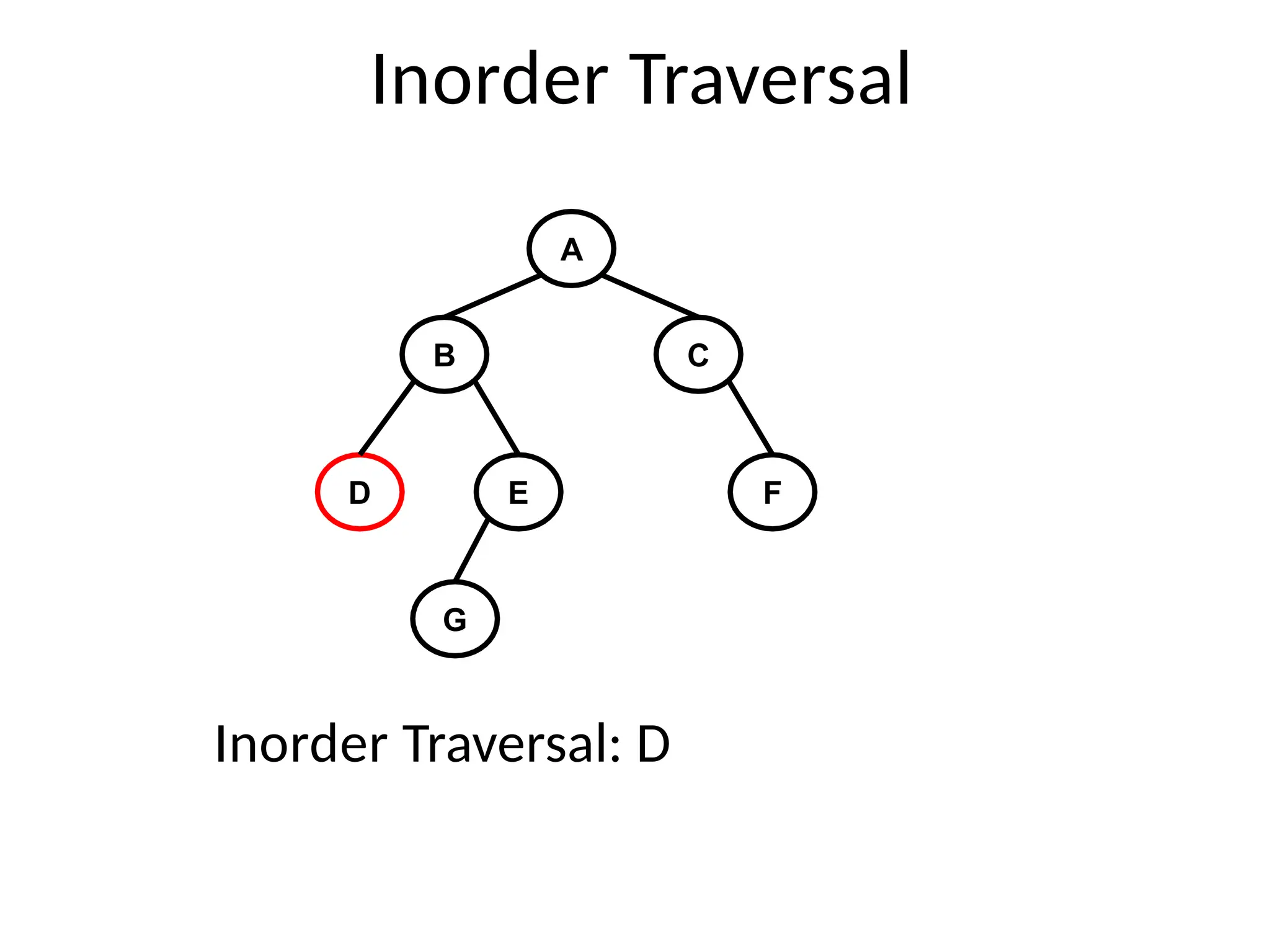
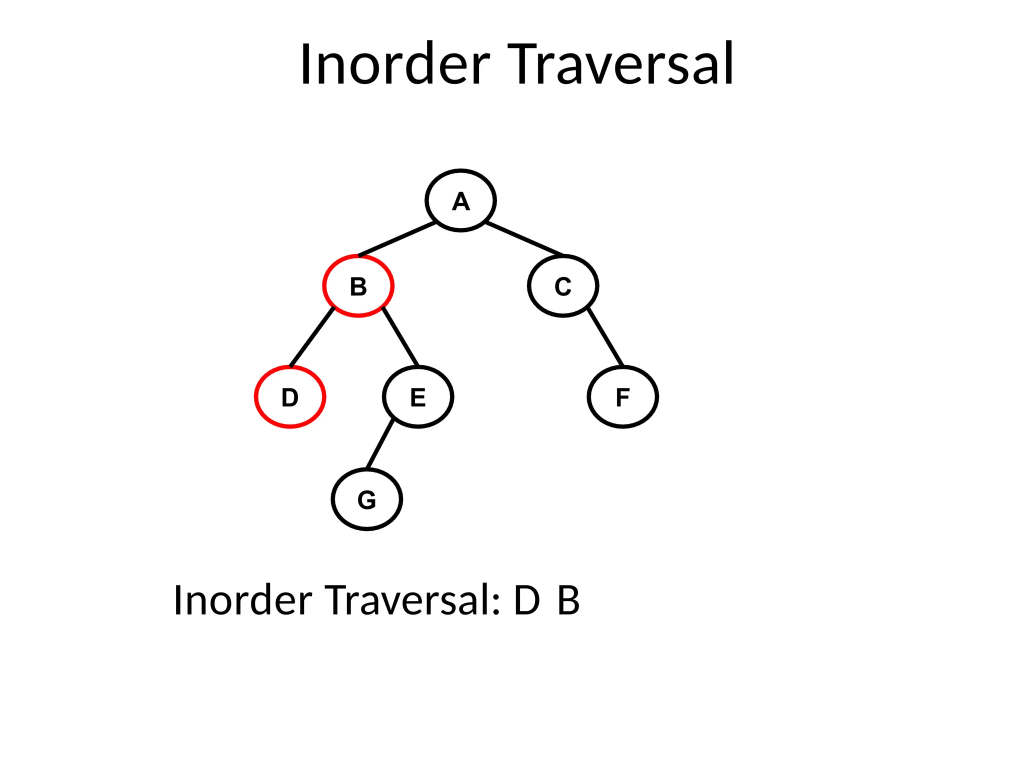
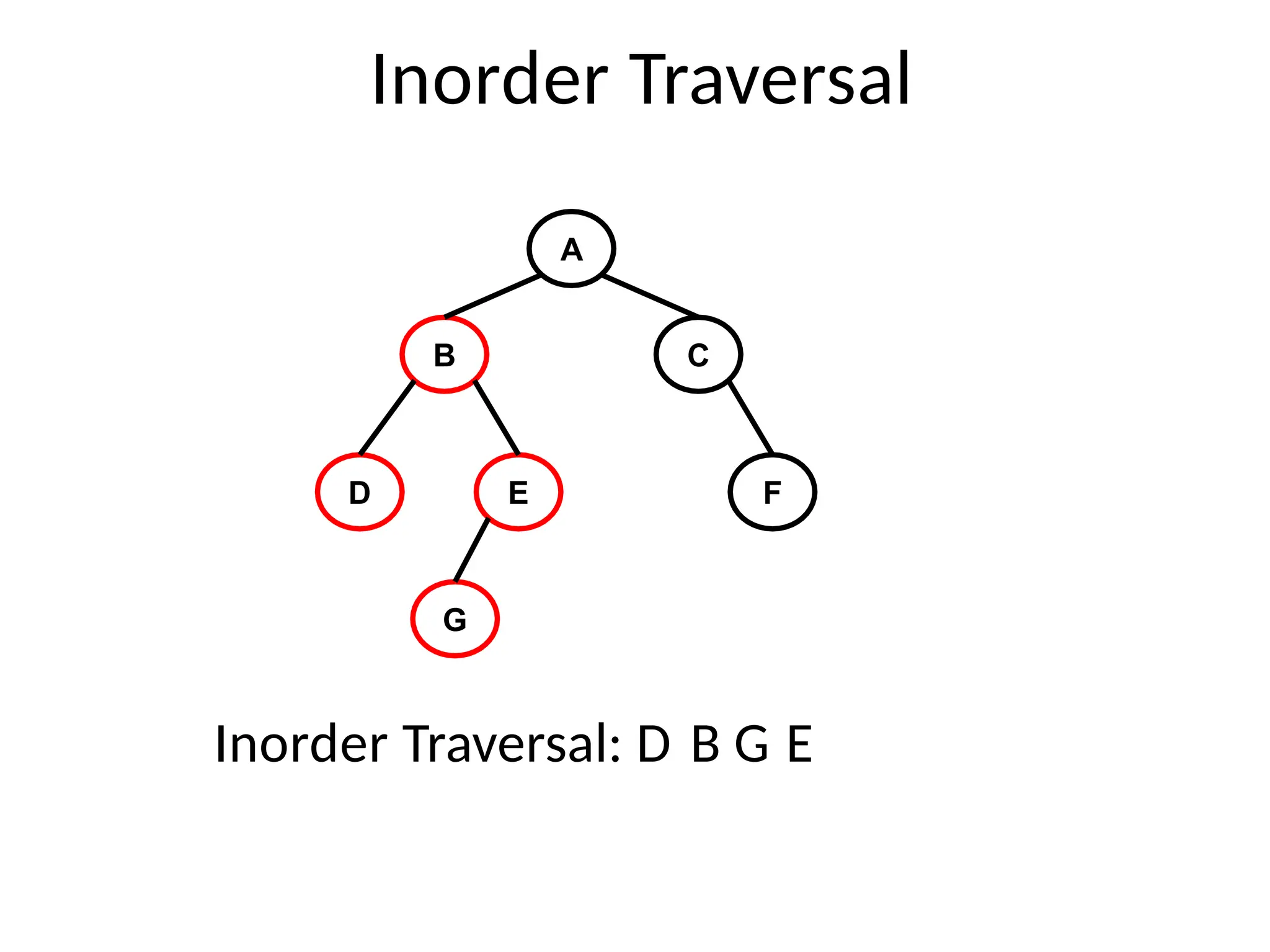
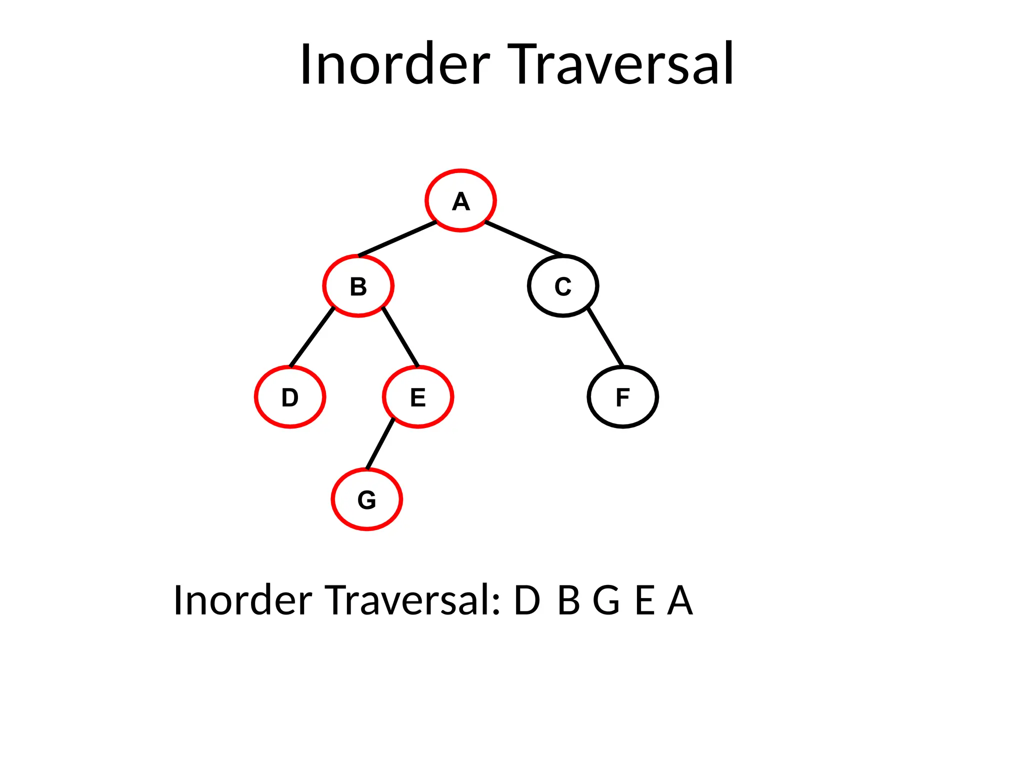
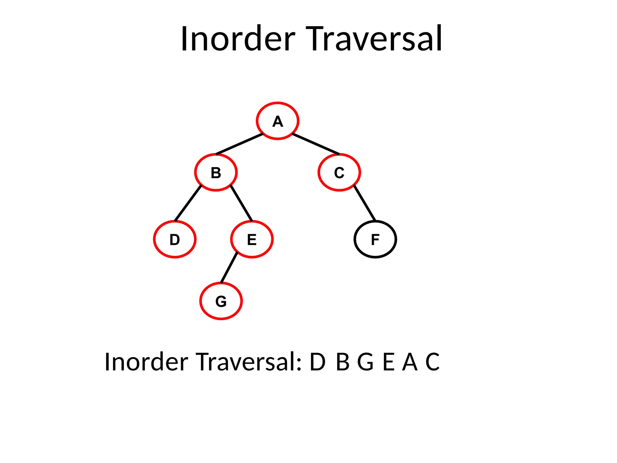
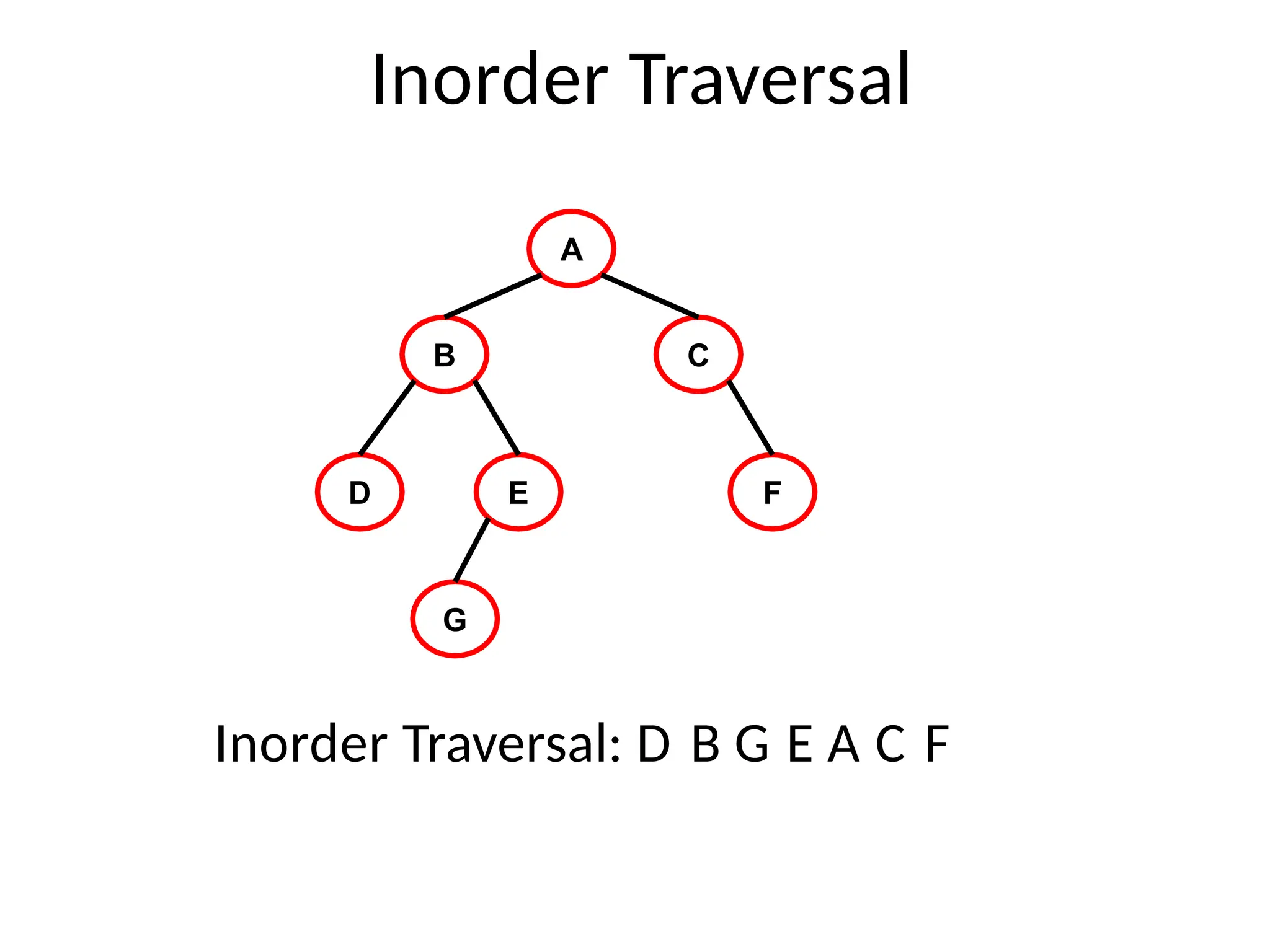
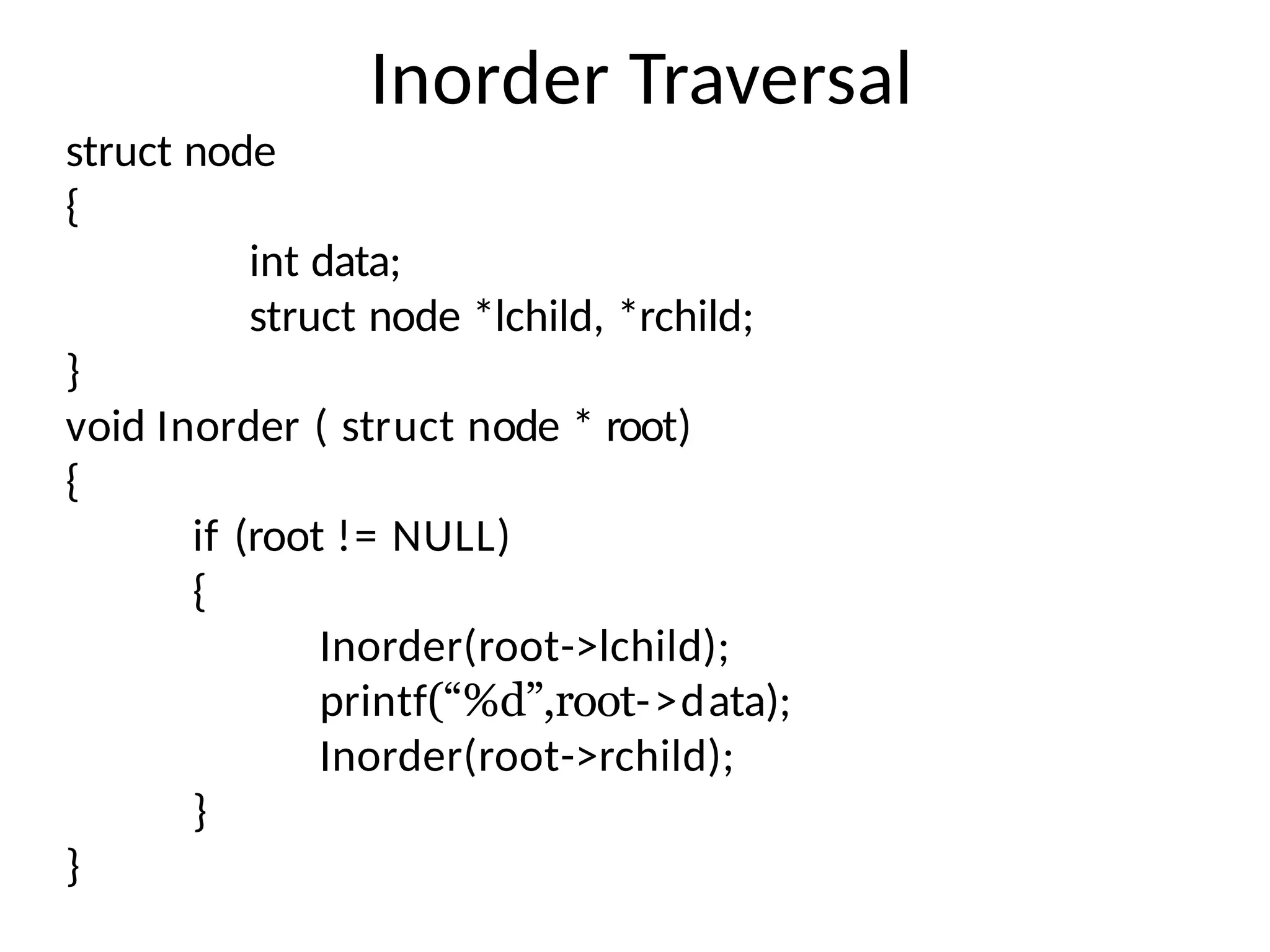
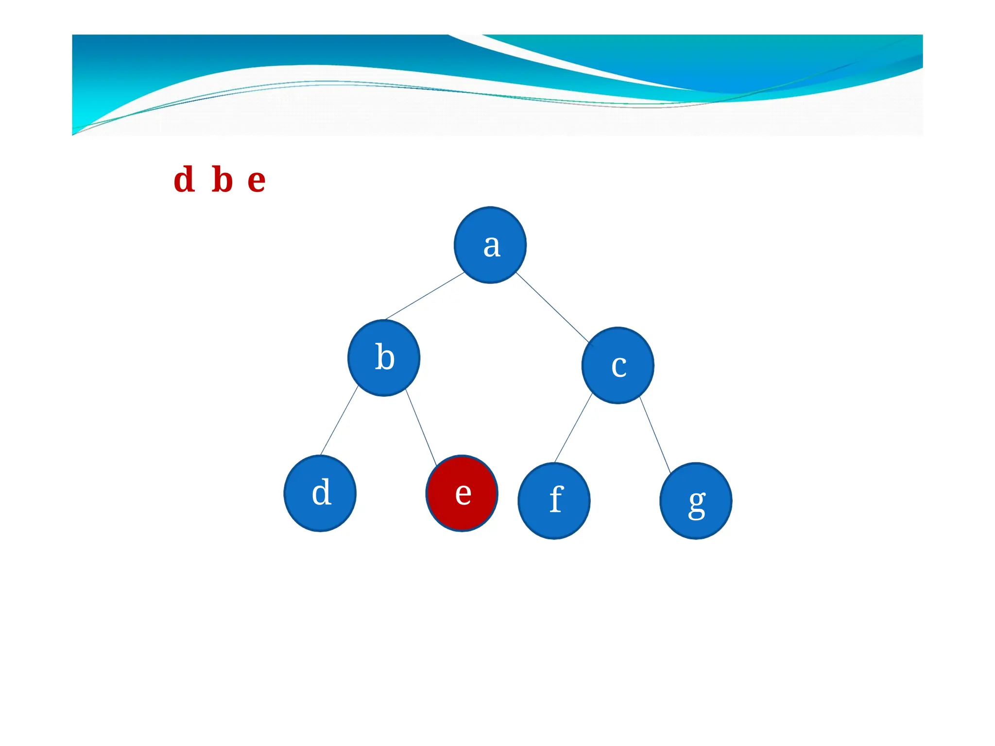
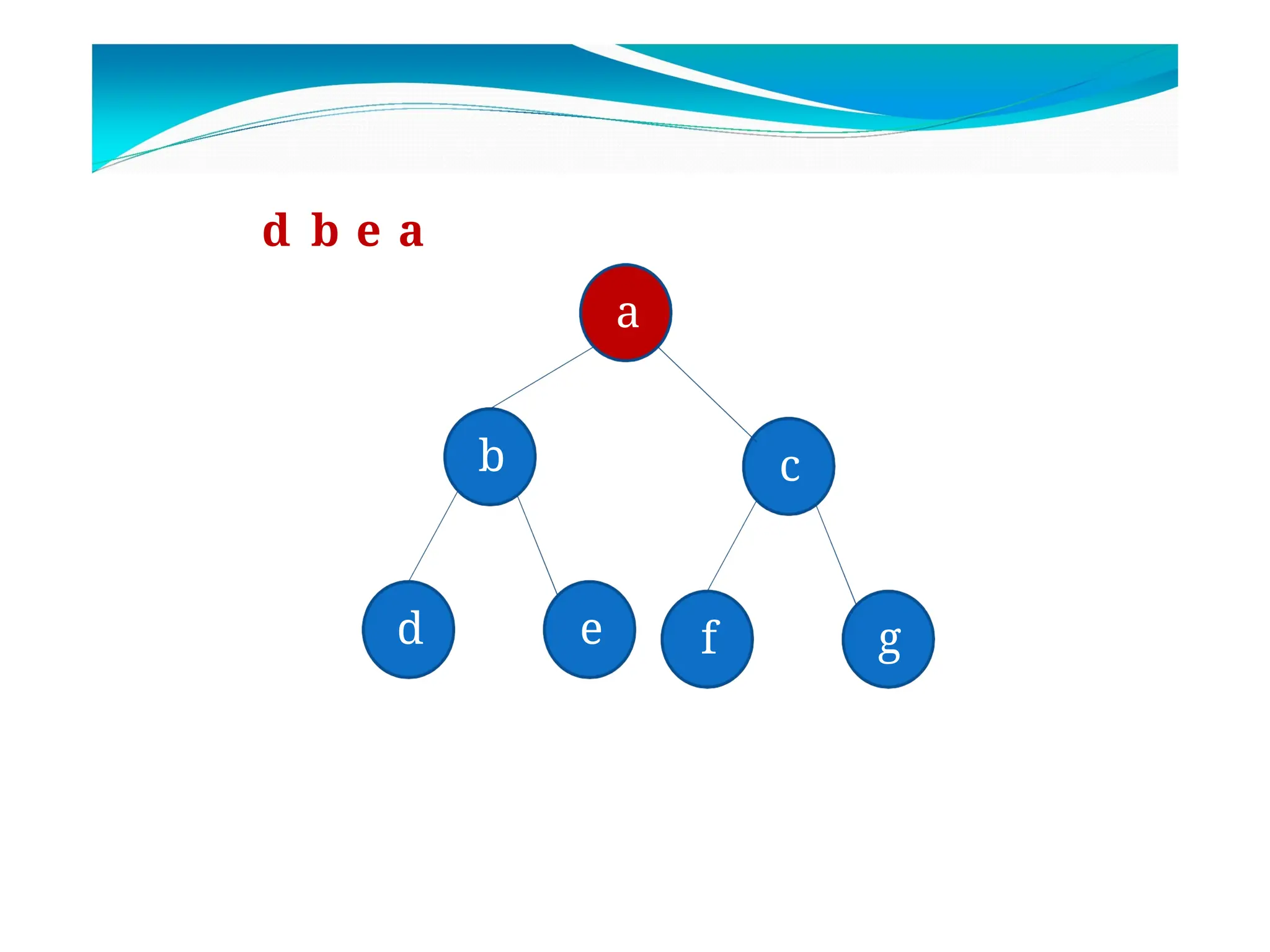
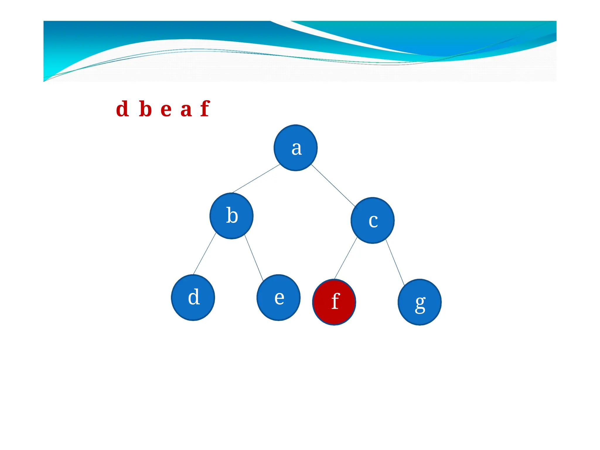
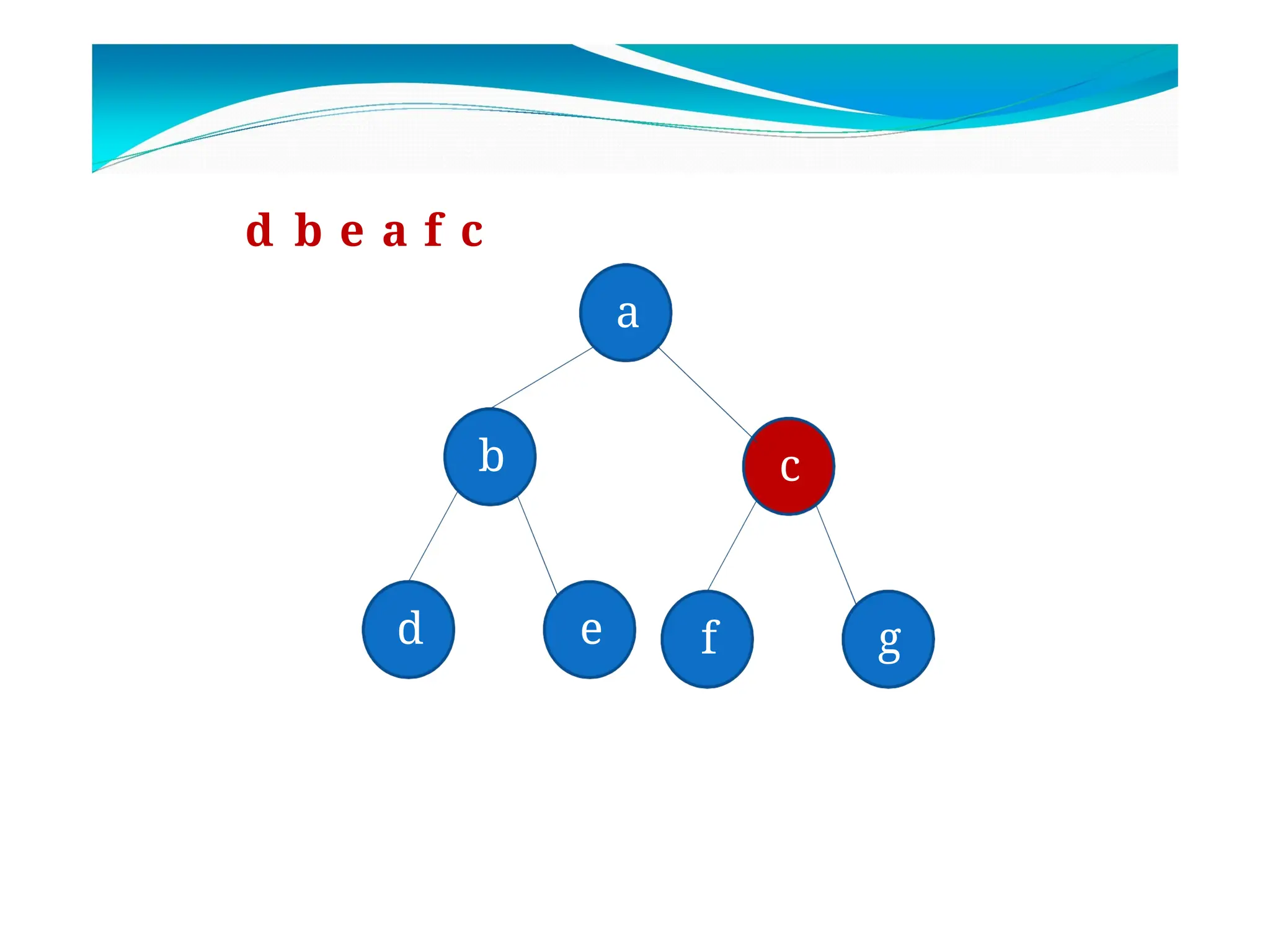
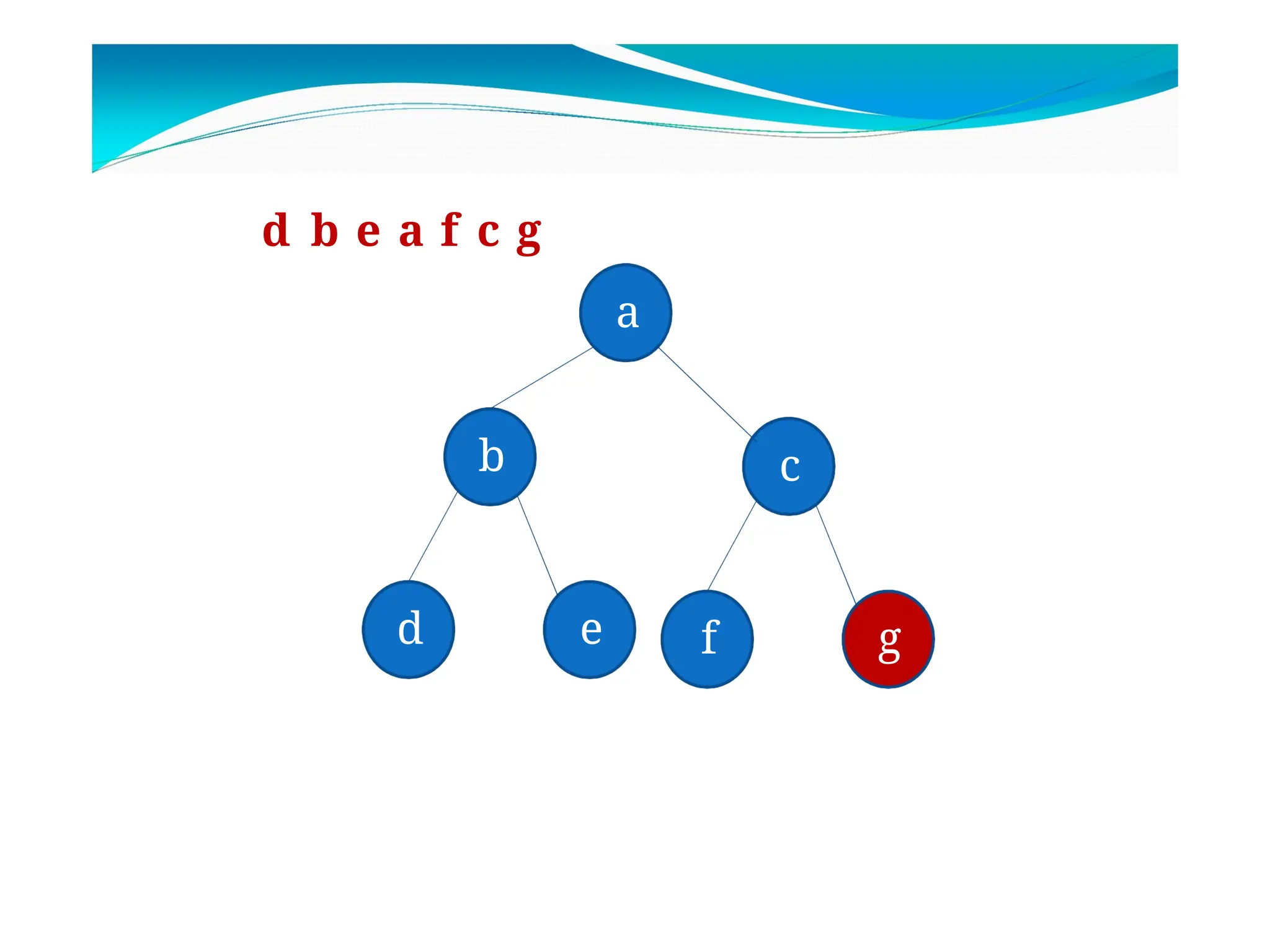
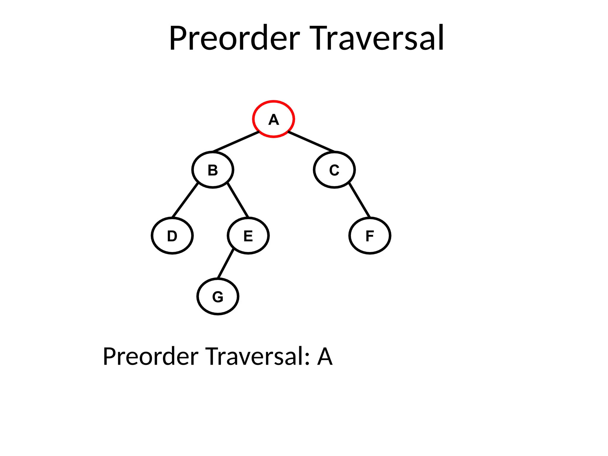
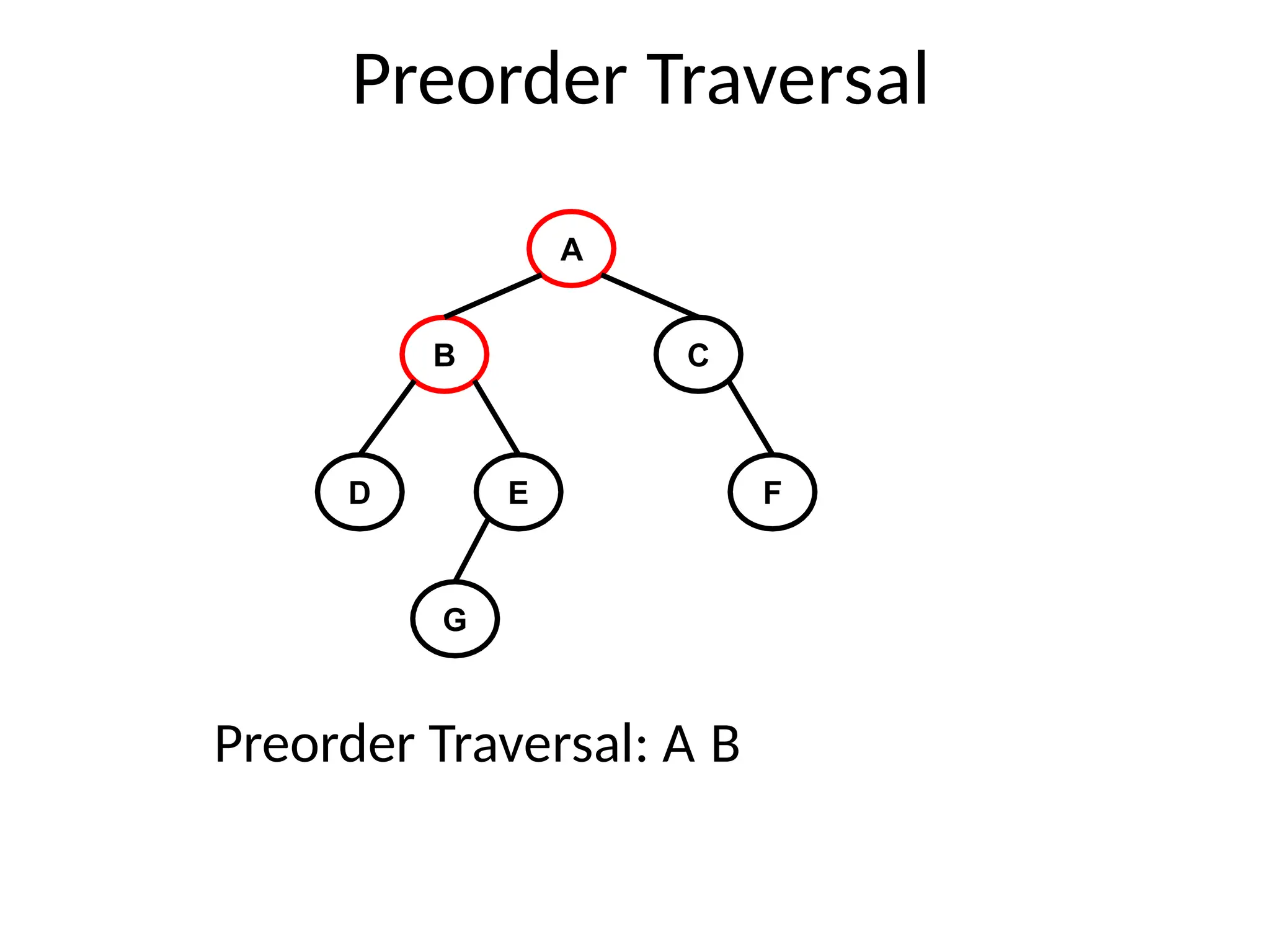
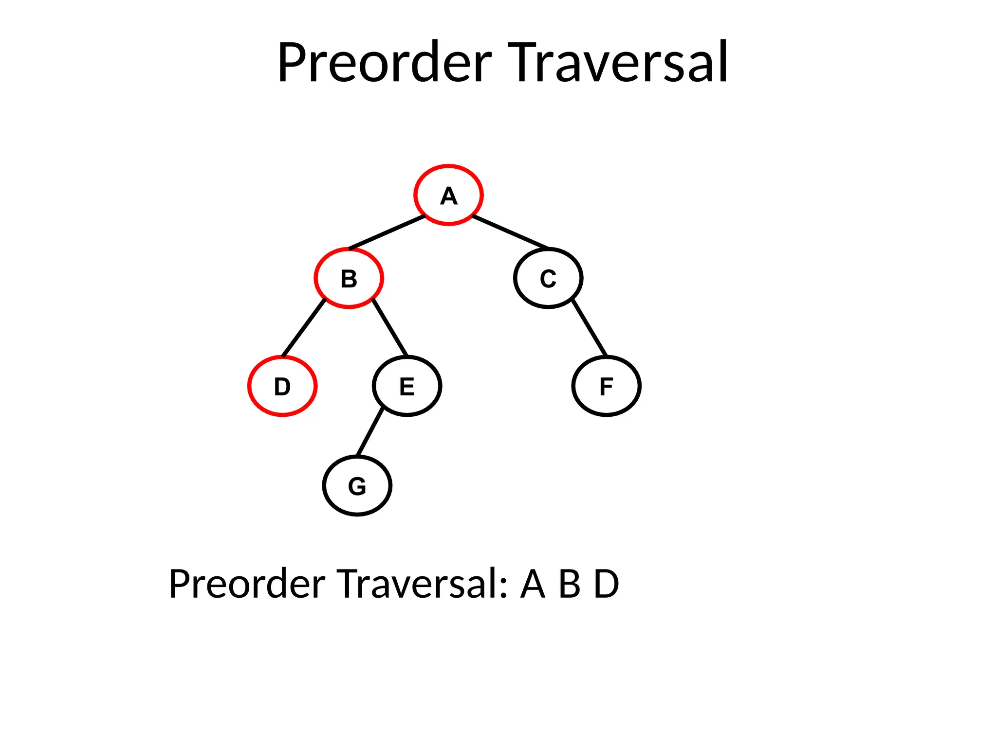
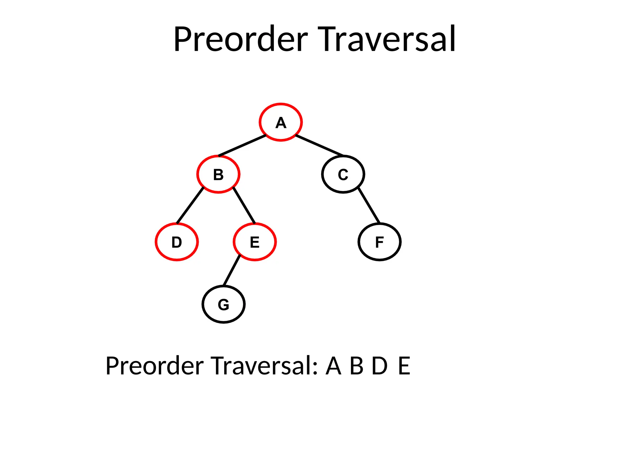
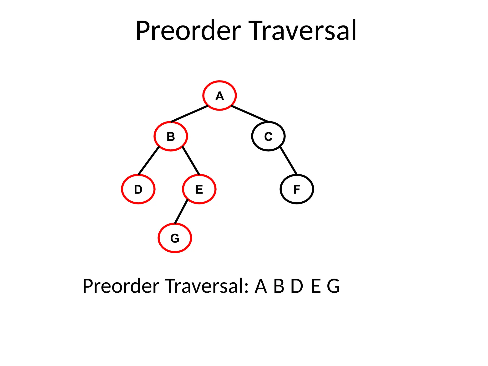
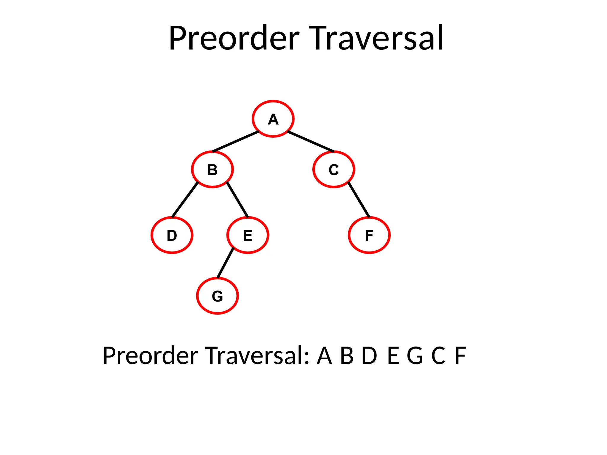
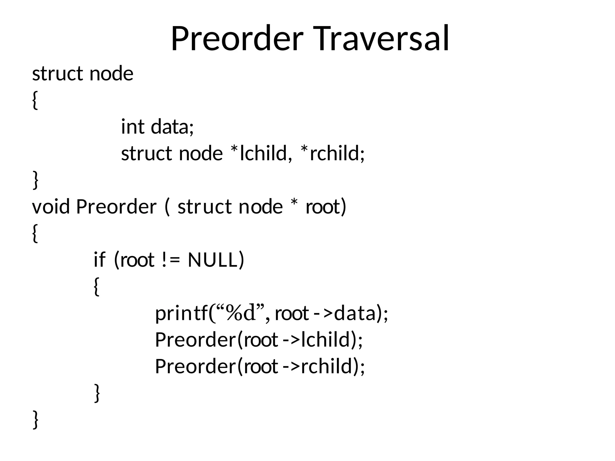
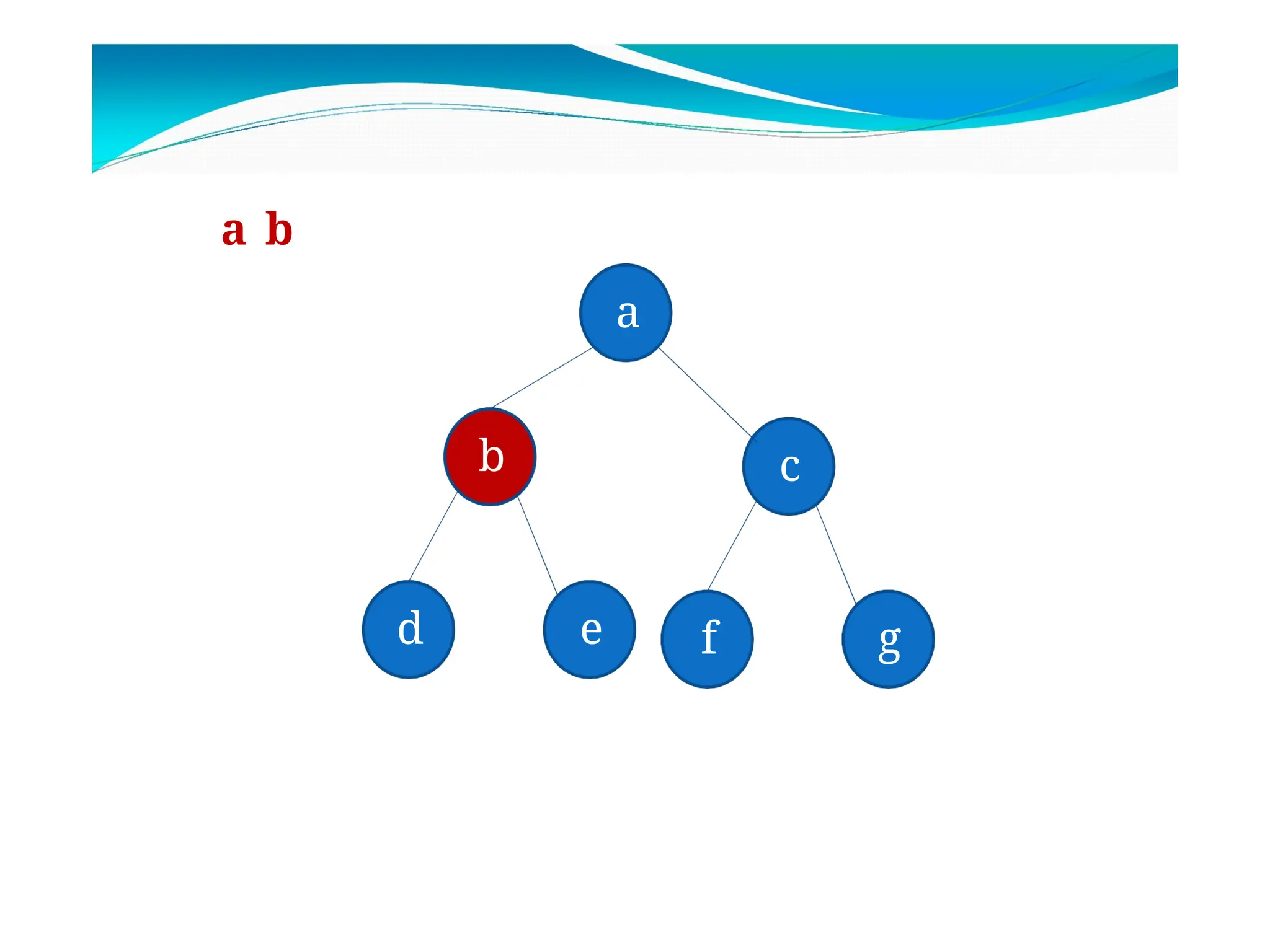
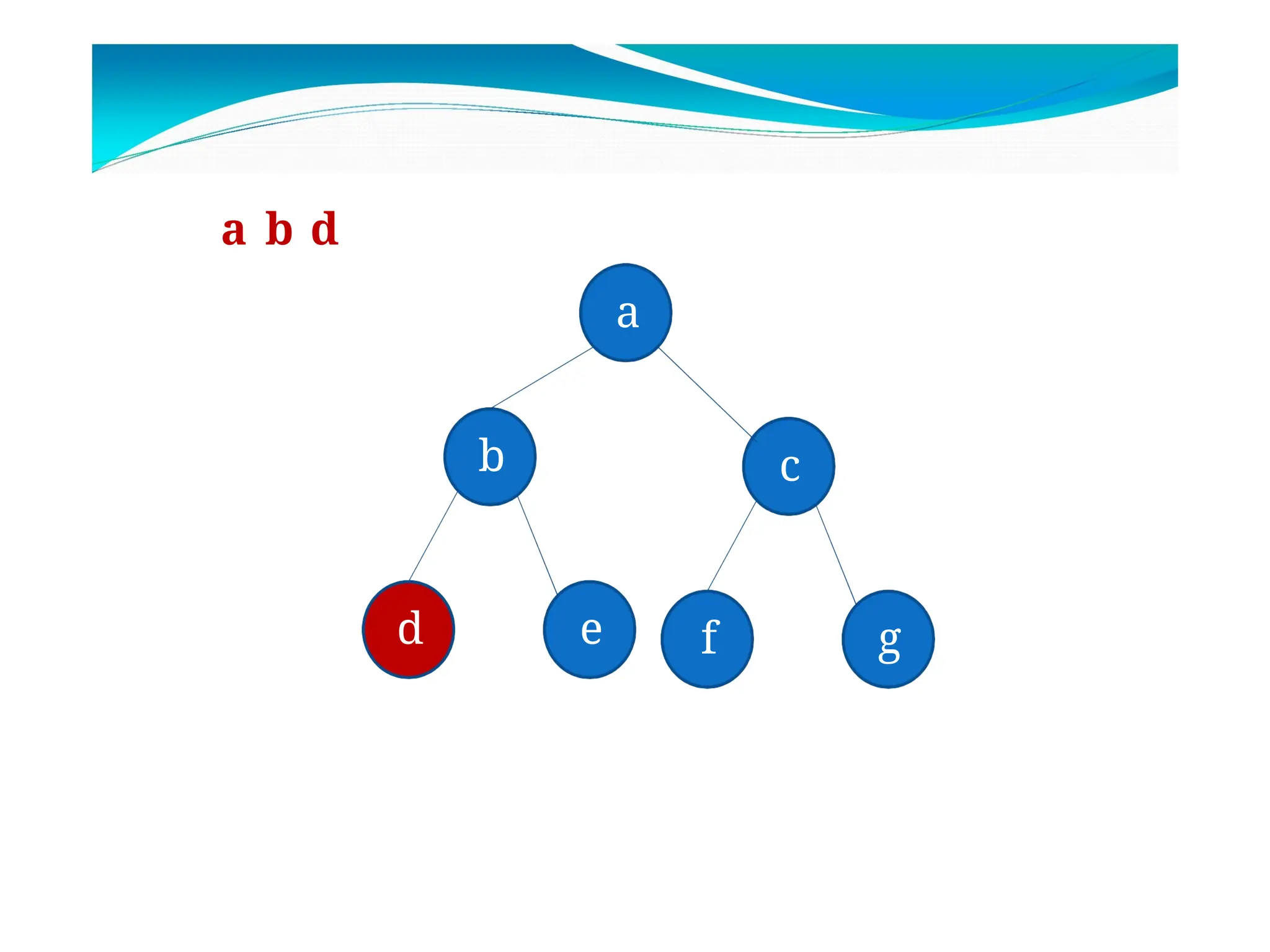
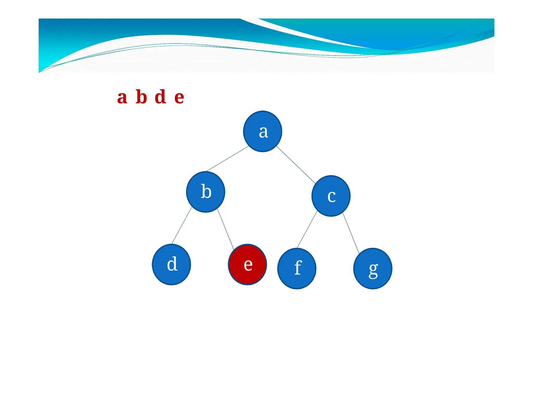
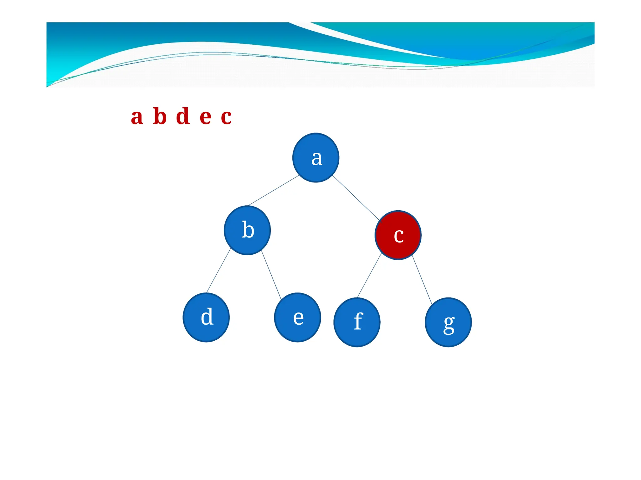
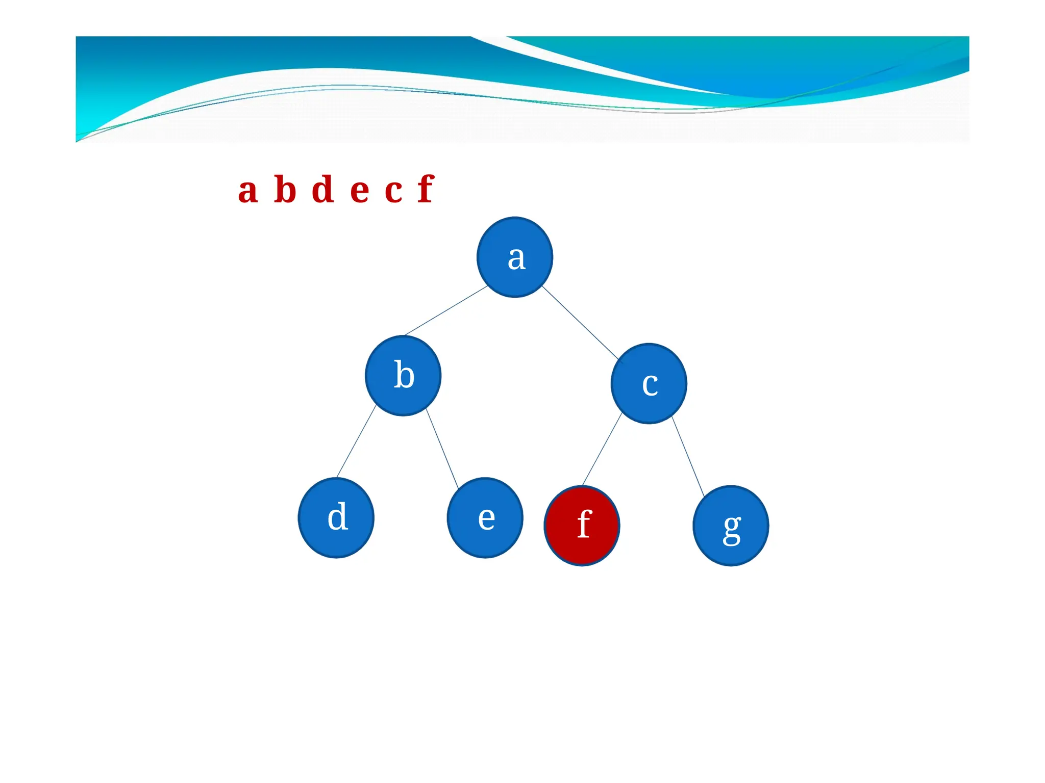
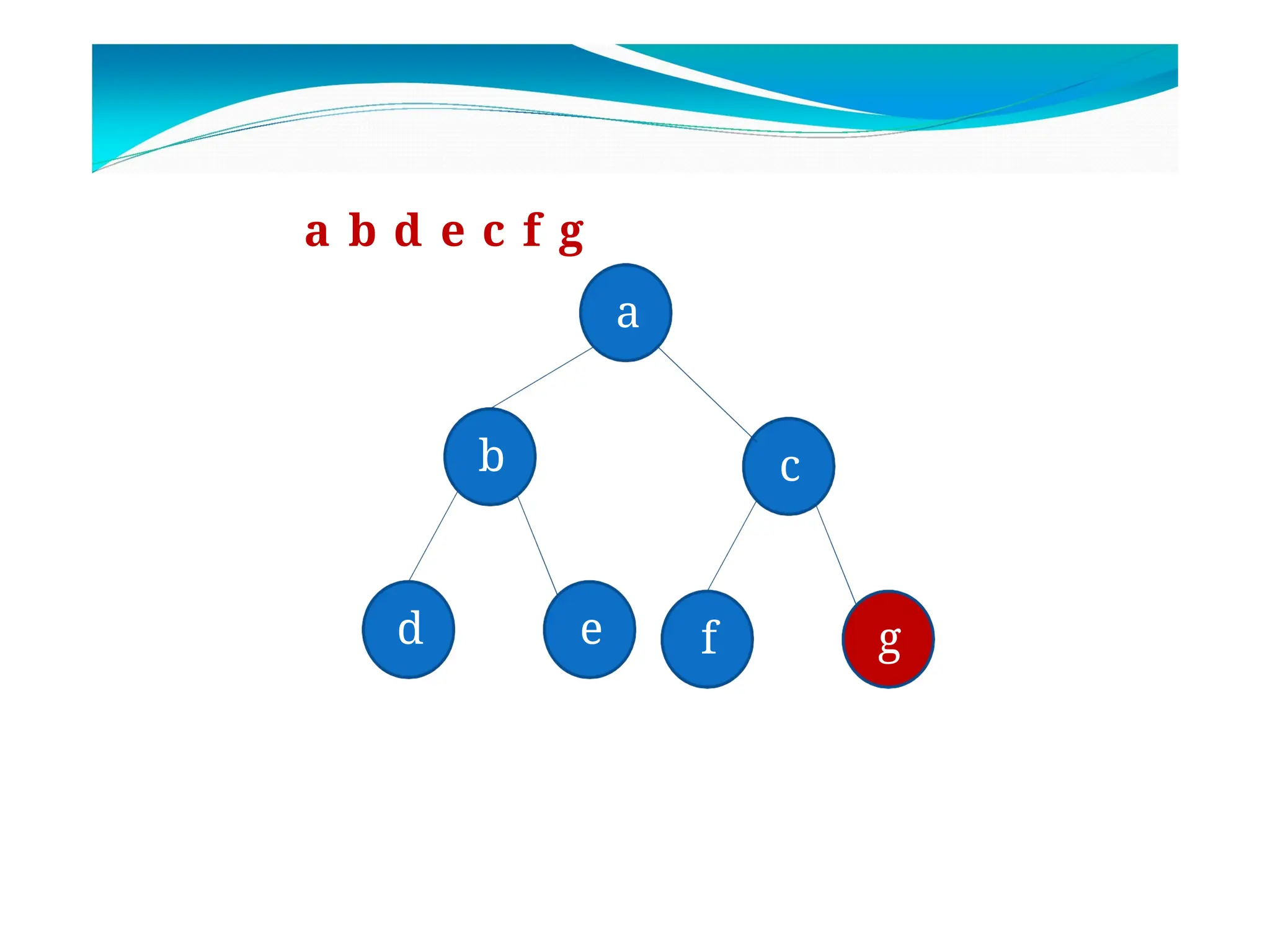
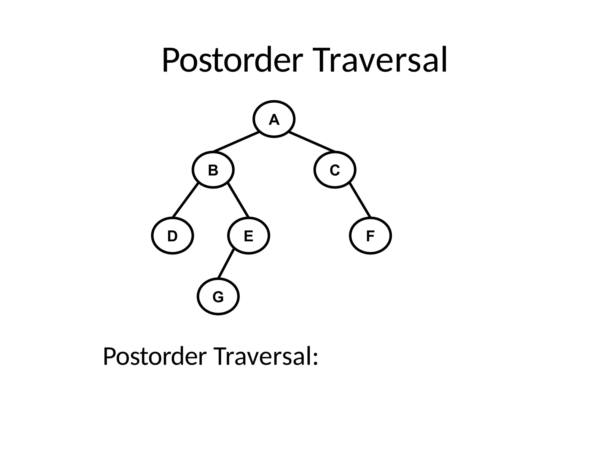
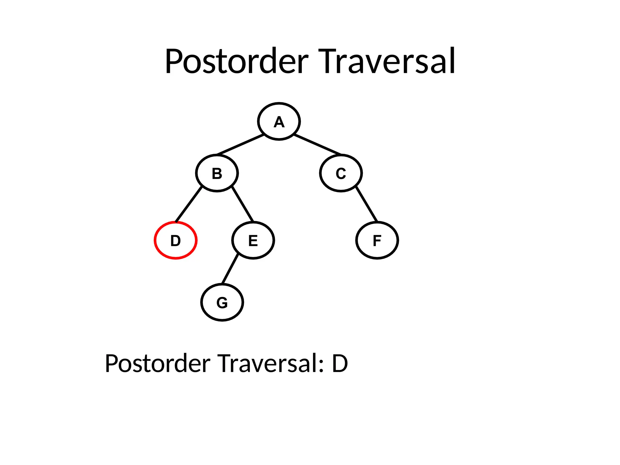
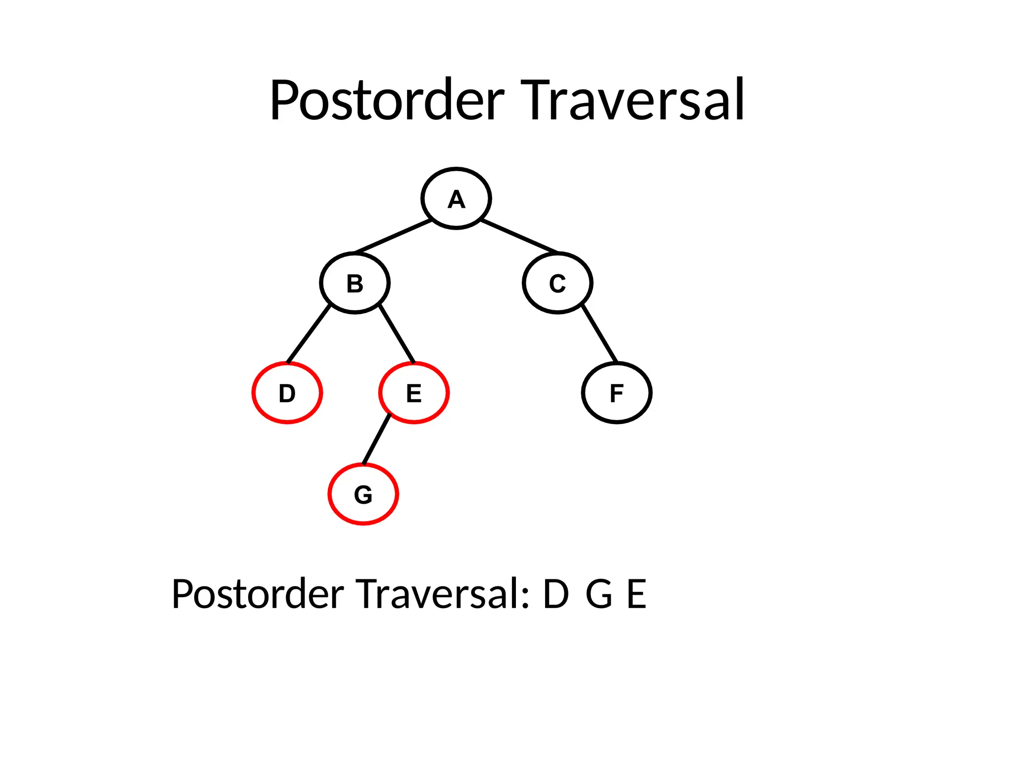
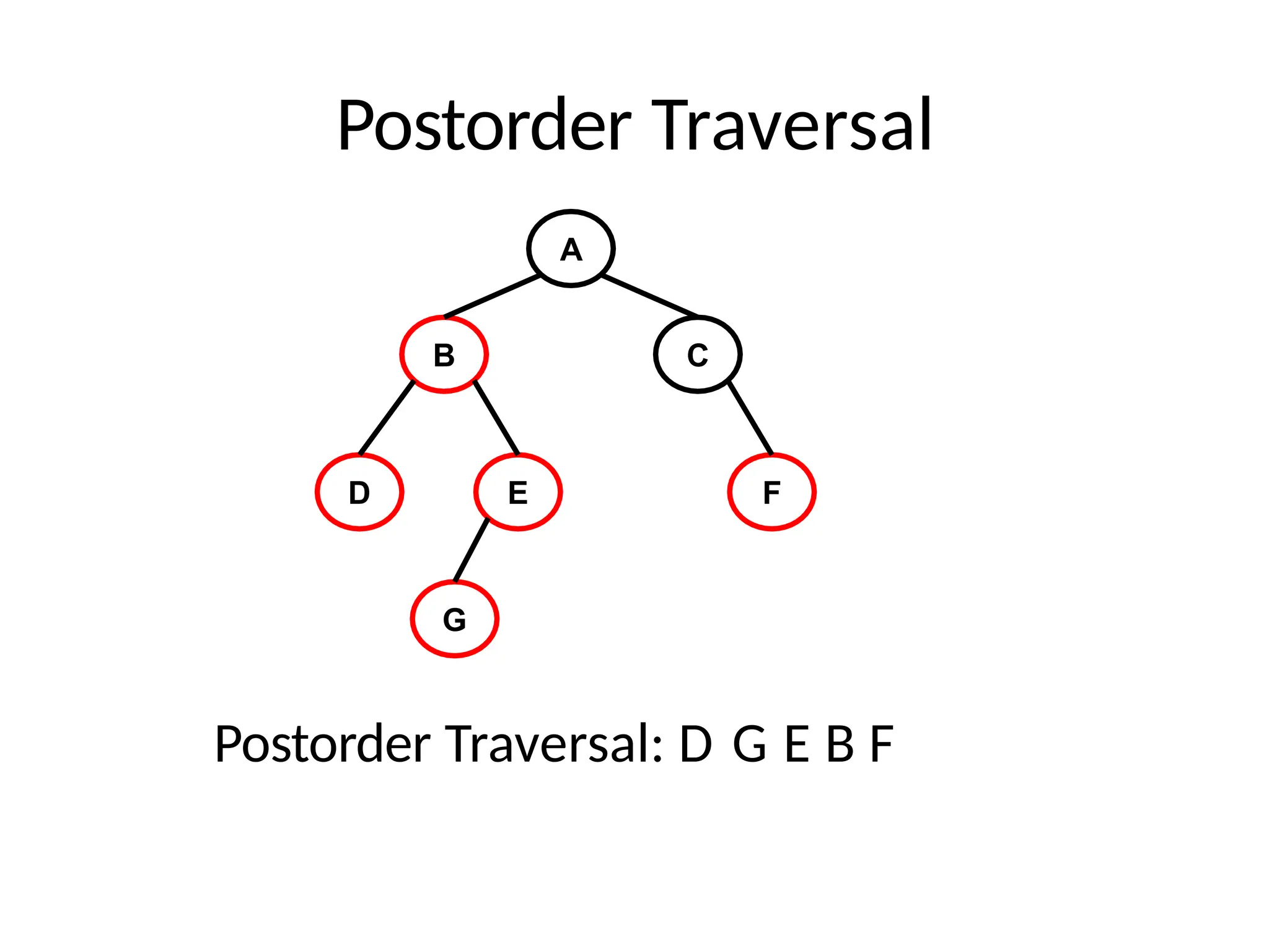
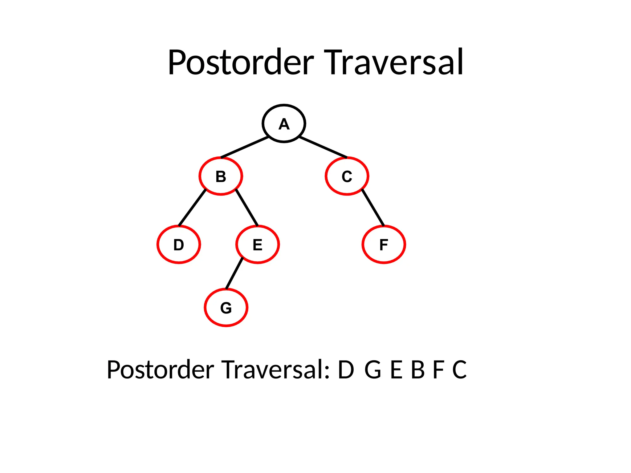
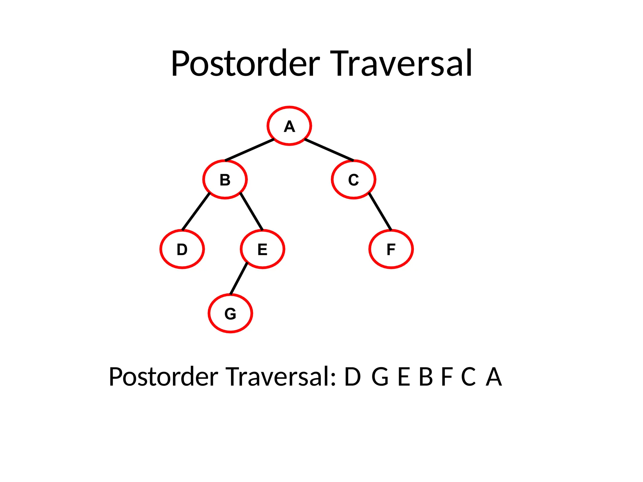
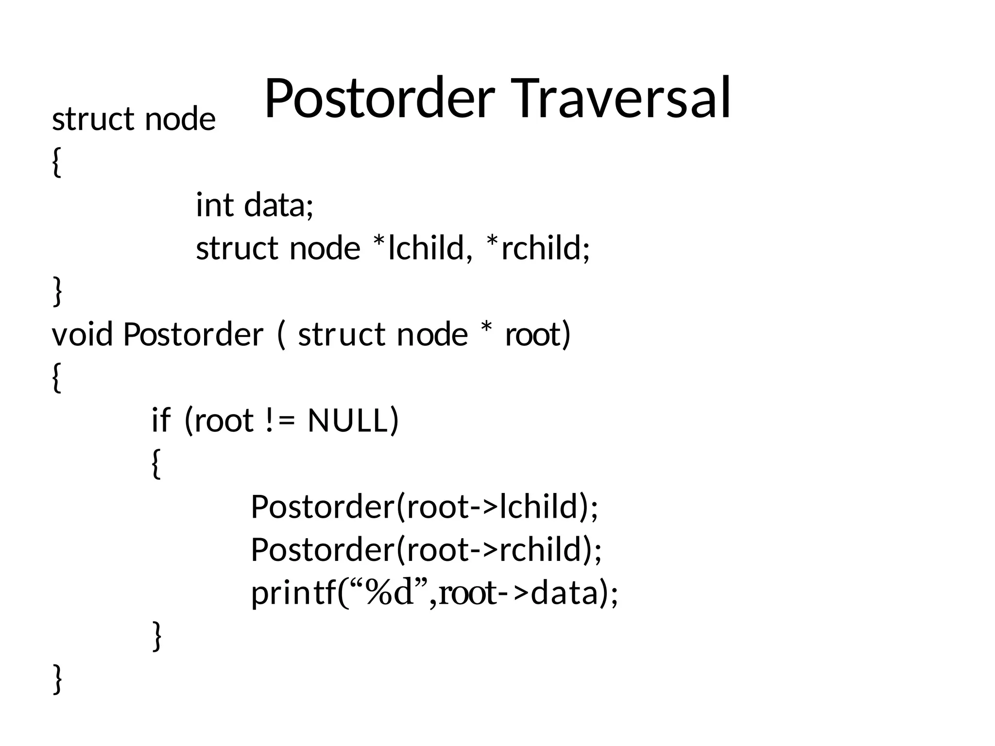
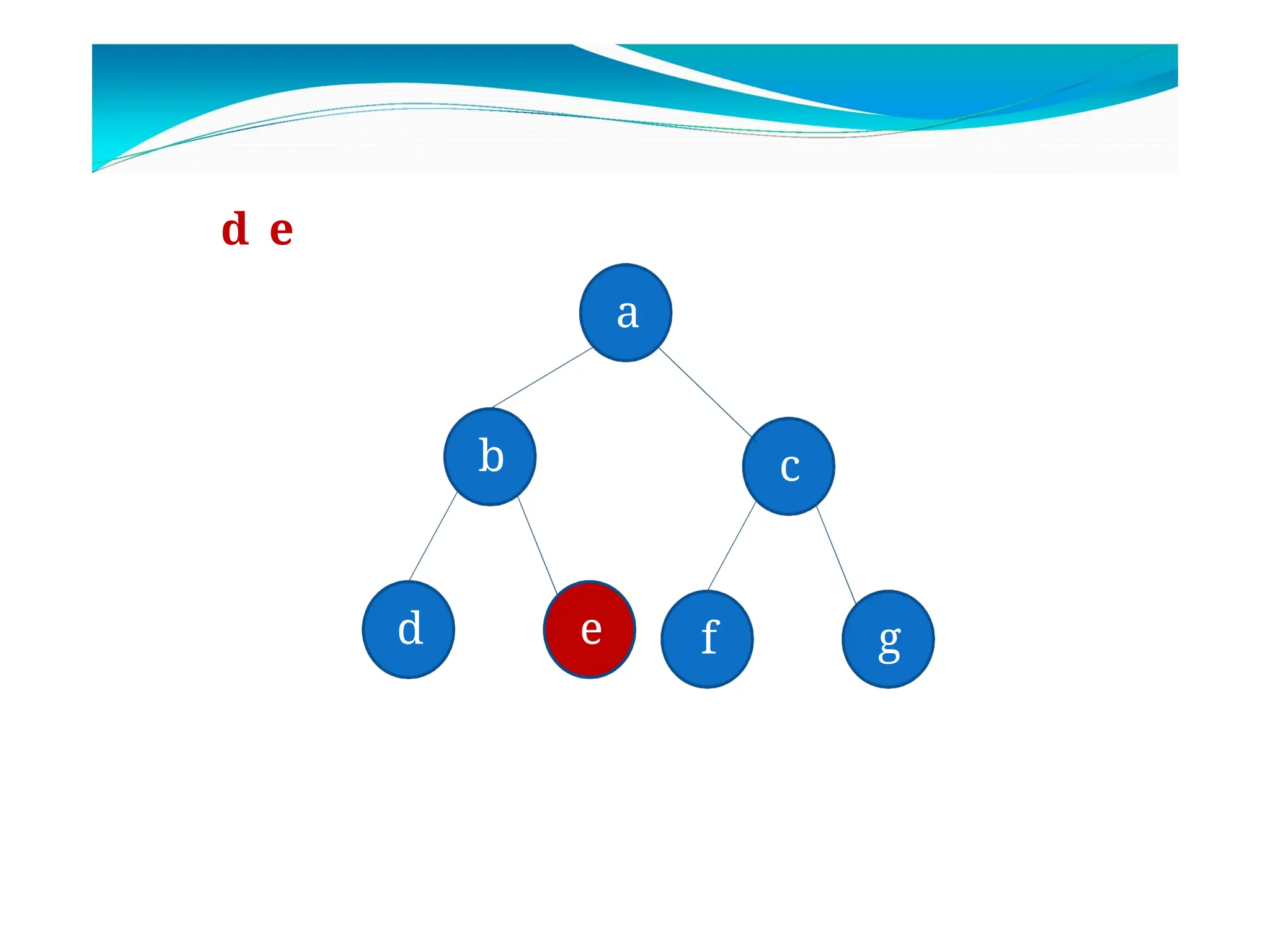
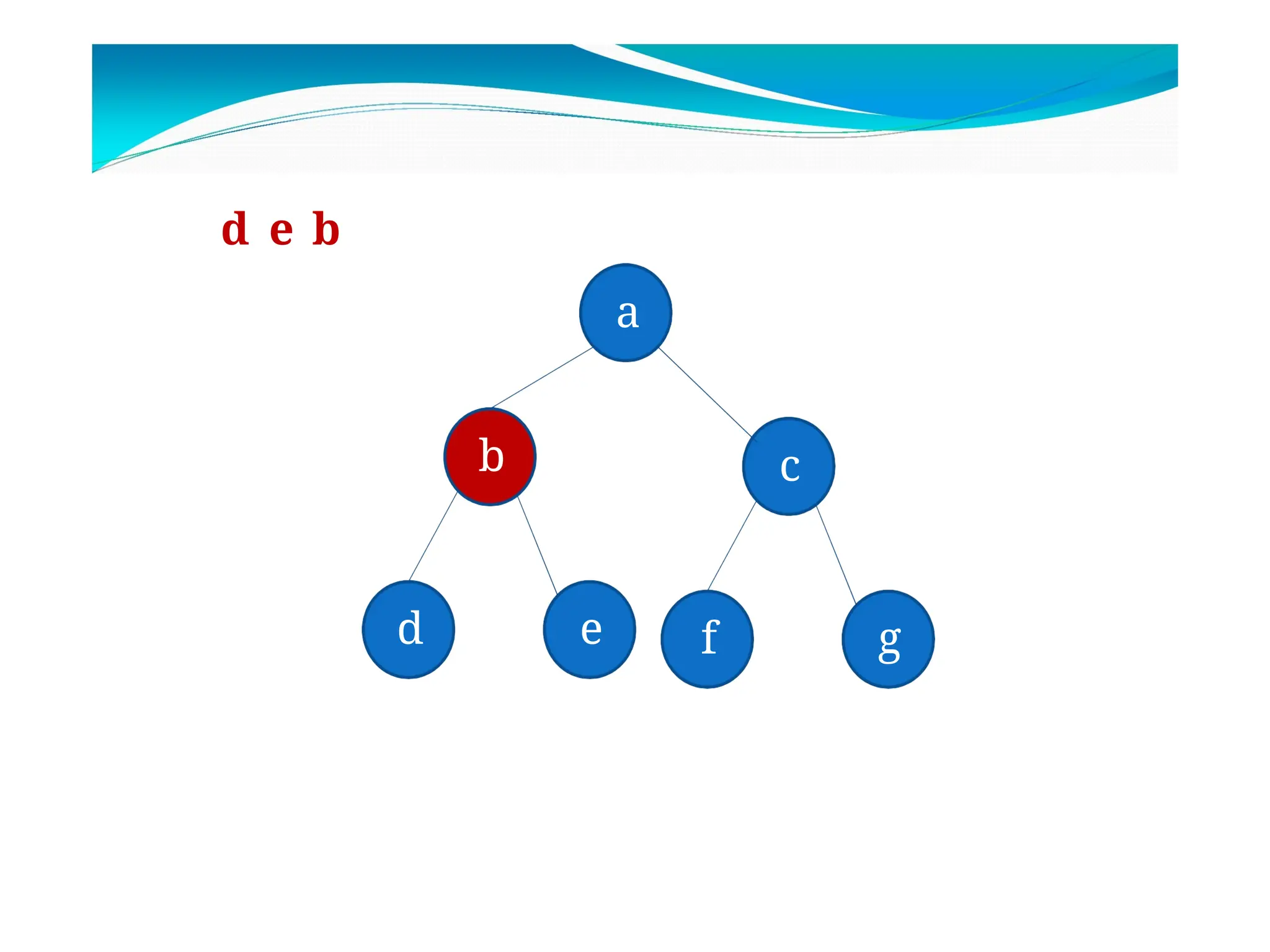
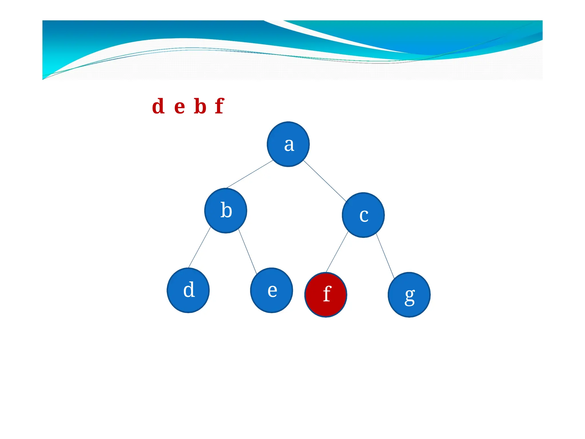
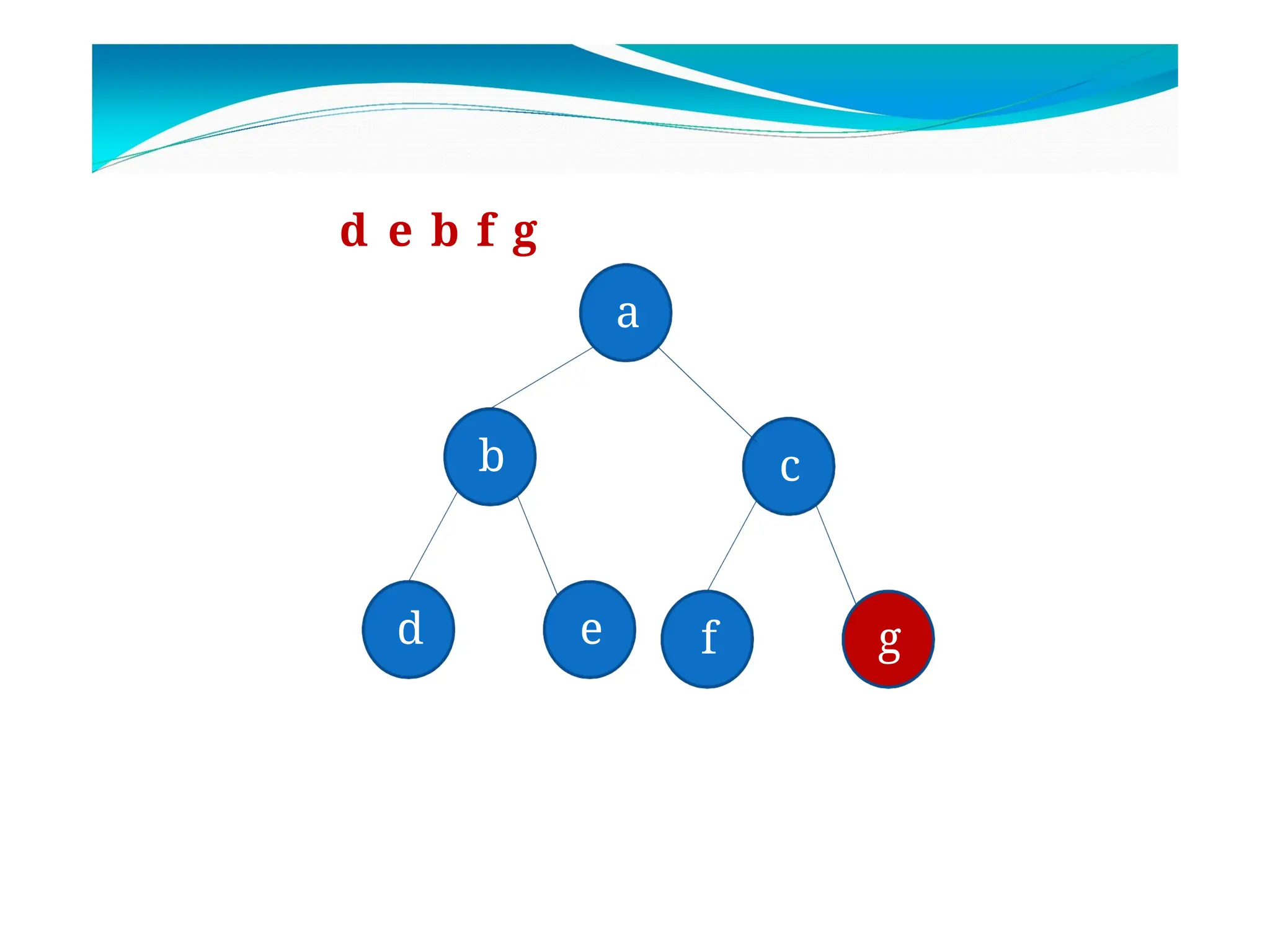
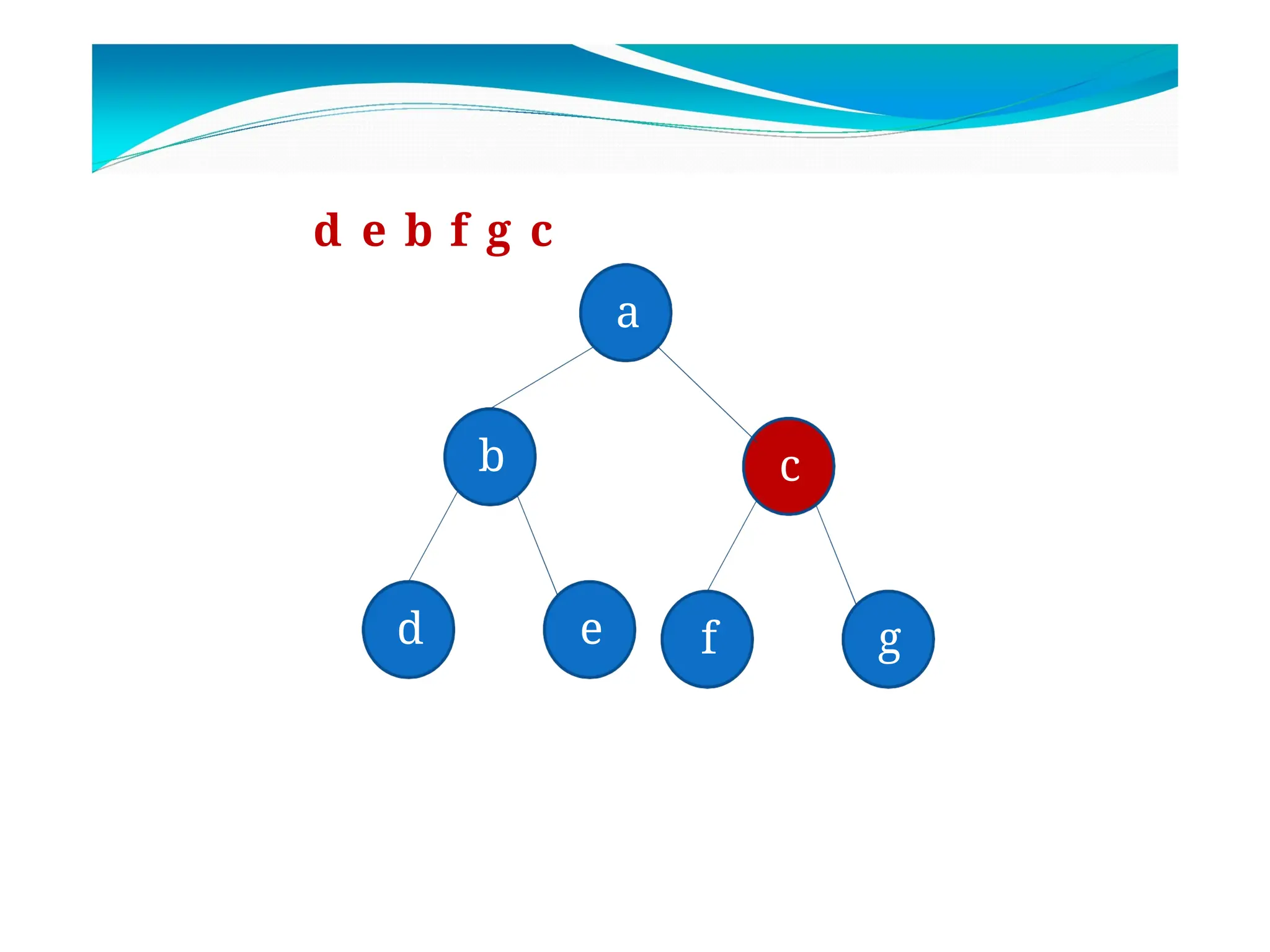
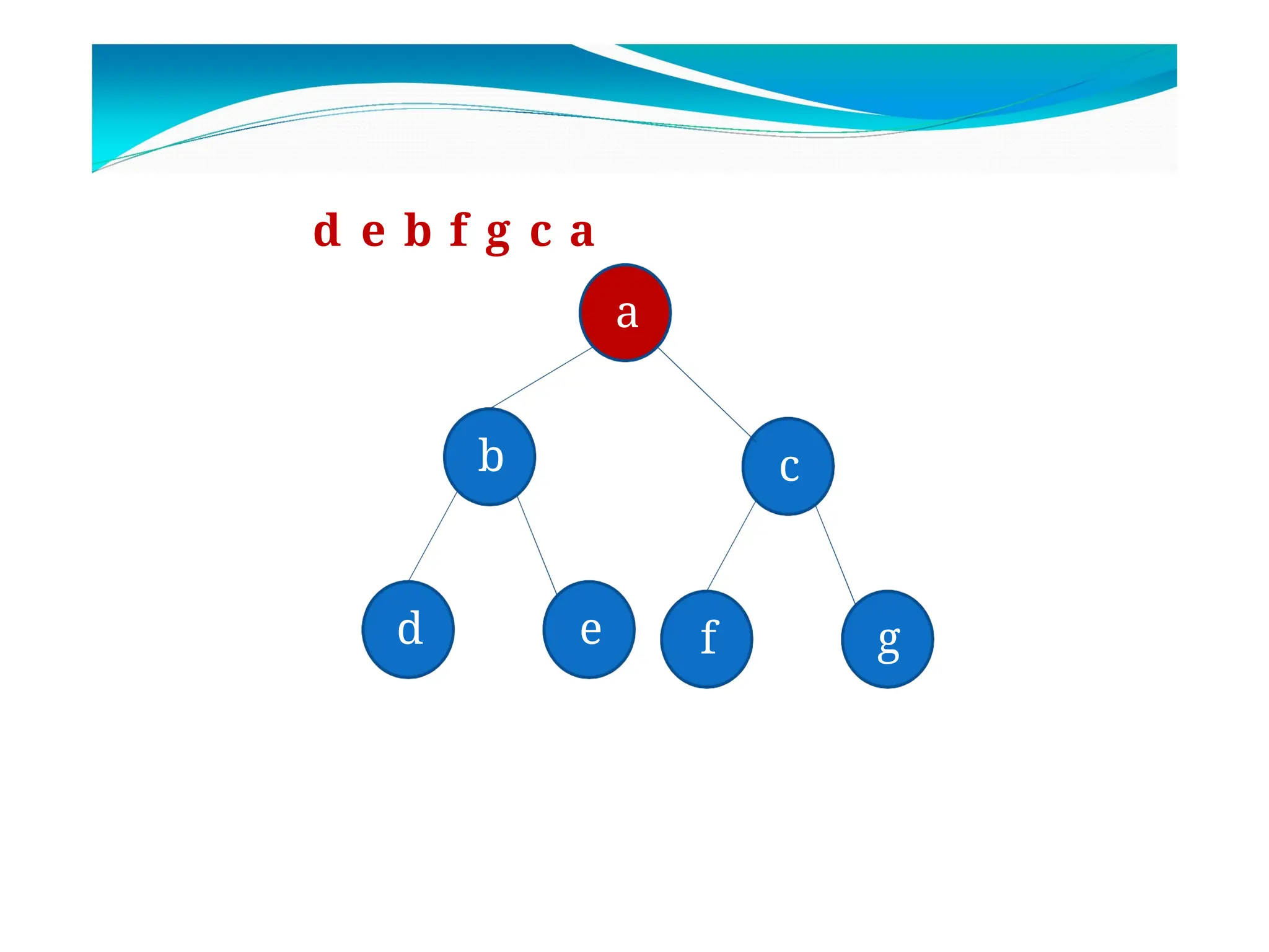
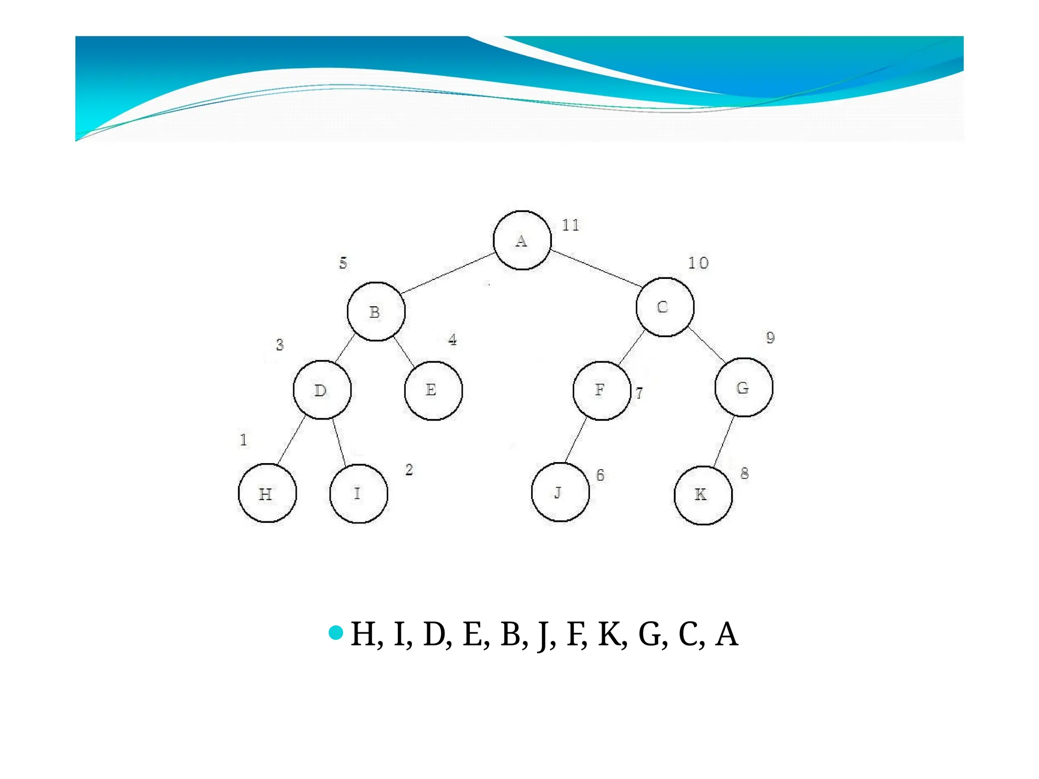
Binary Tree Traversals
Traversal means visit each node in the
binary tree exactly once
There are three commonly used tree traversals
Inoder Traversal
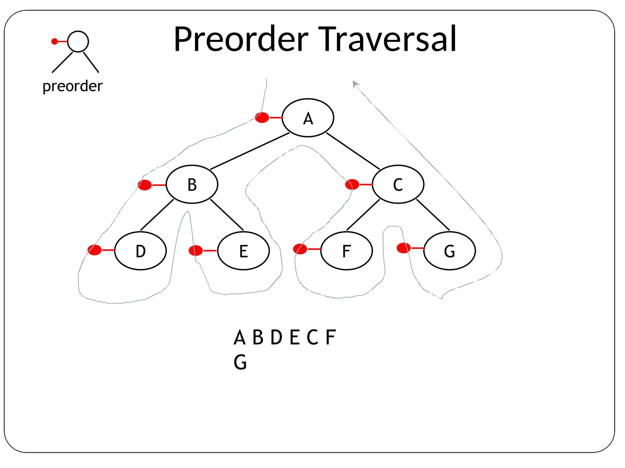
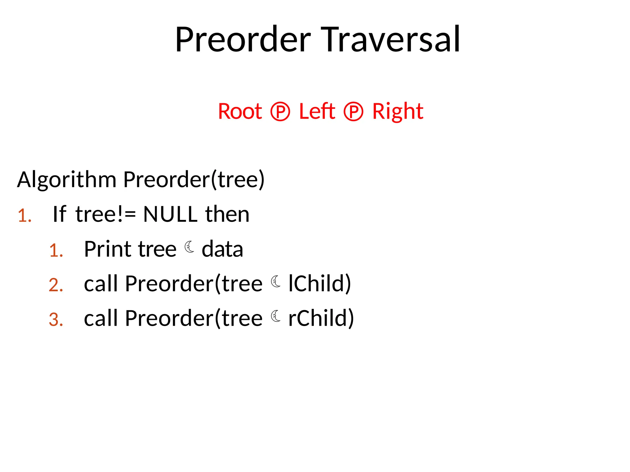
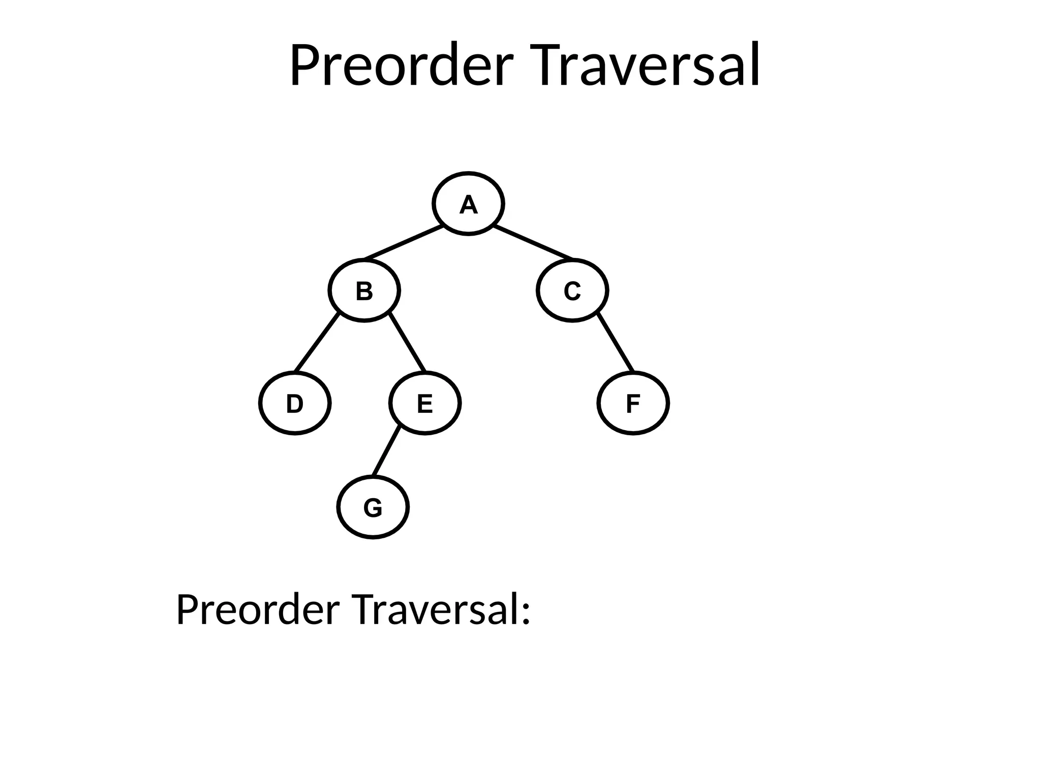
Preorder Traversal
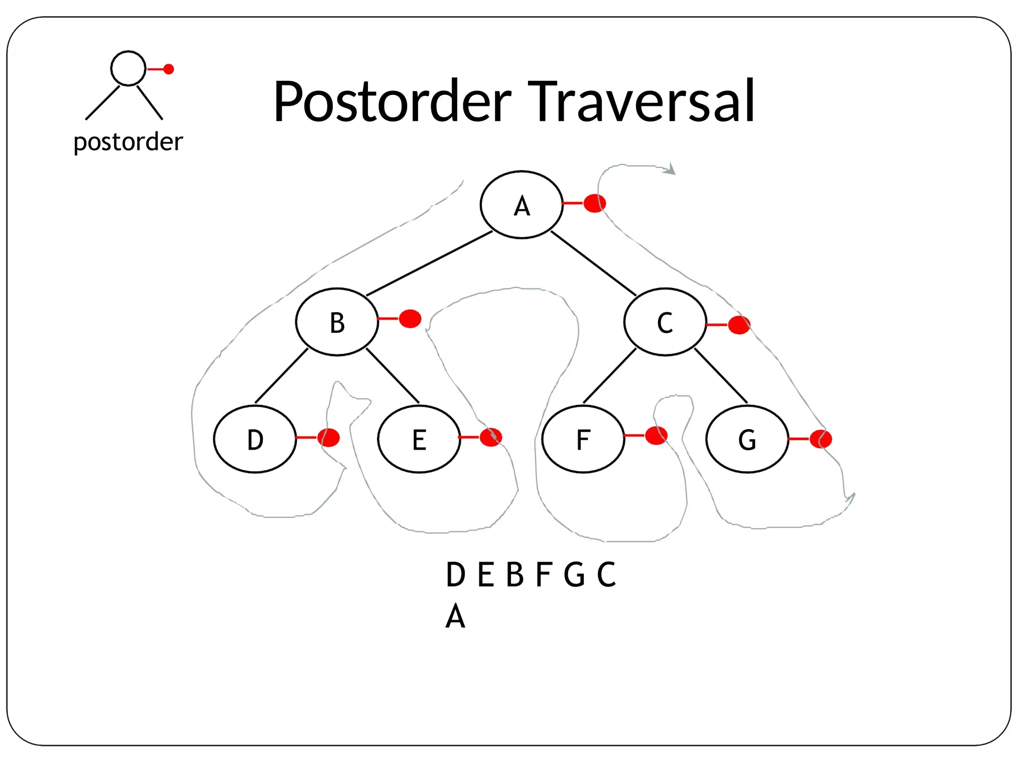
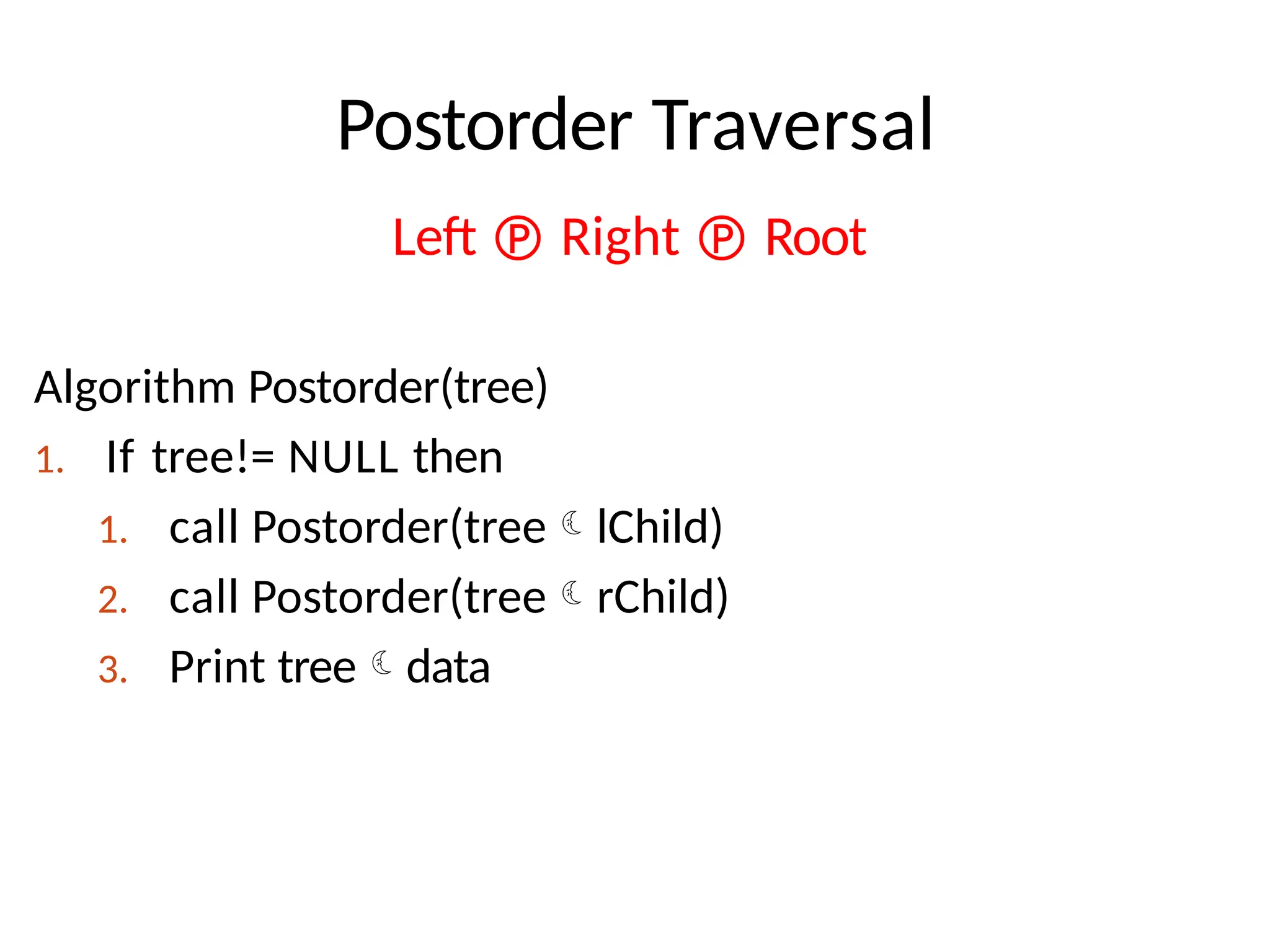
Postorder Traversal
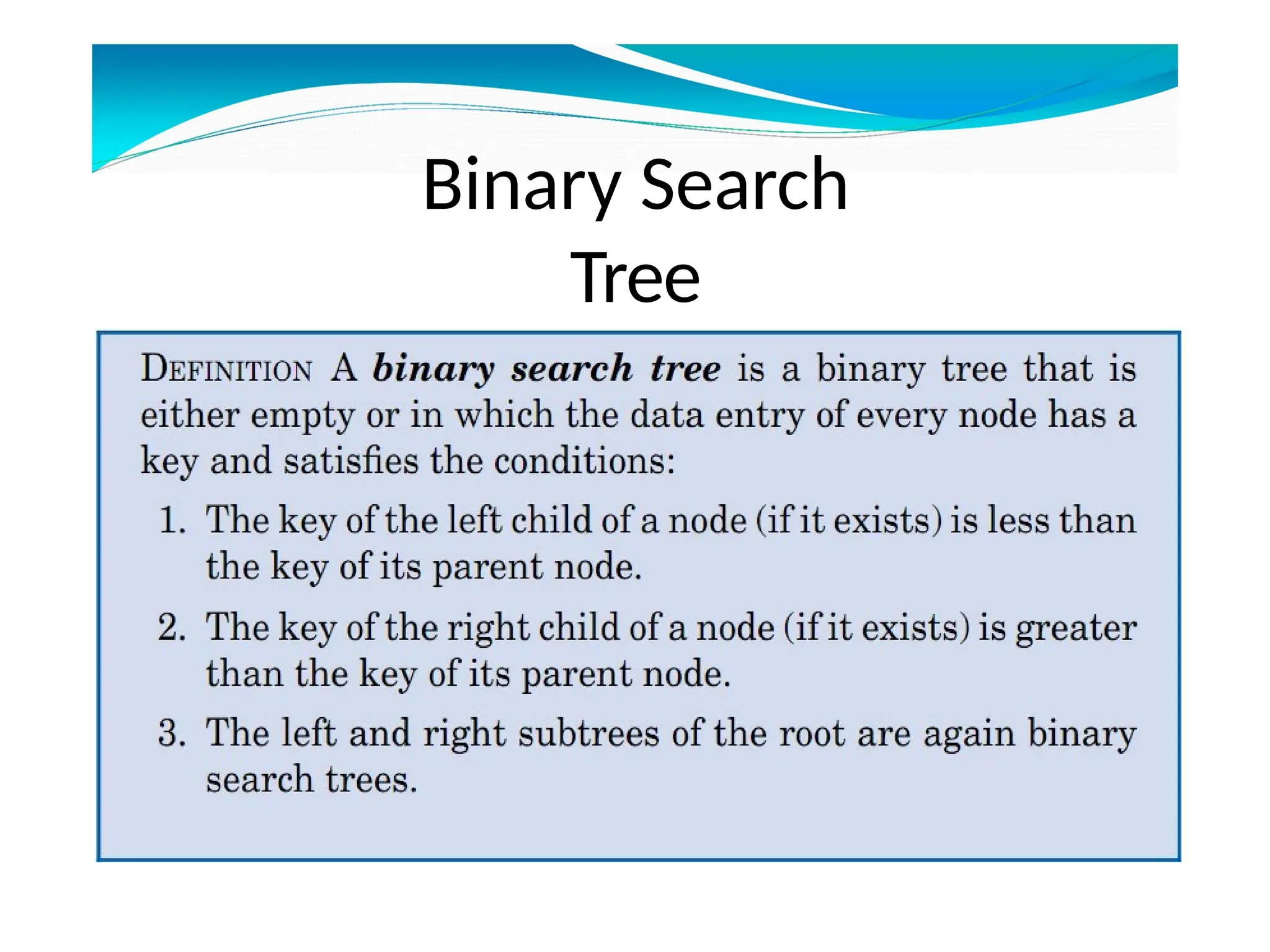
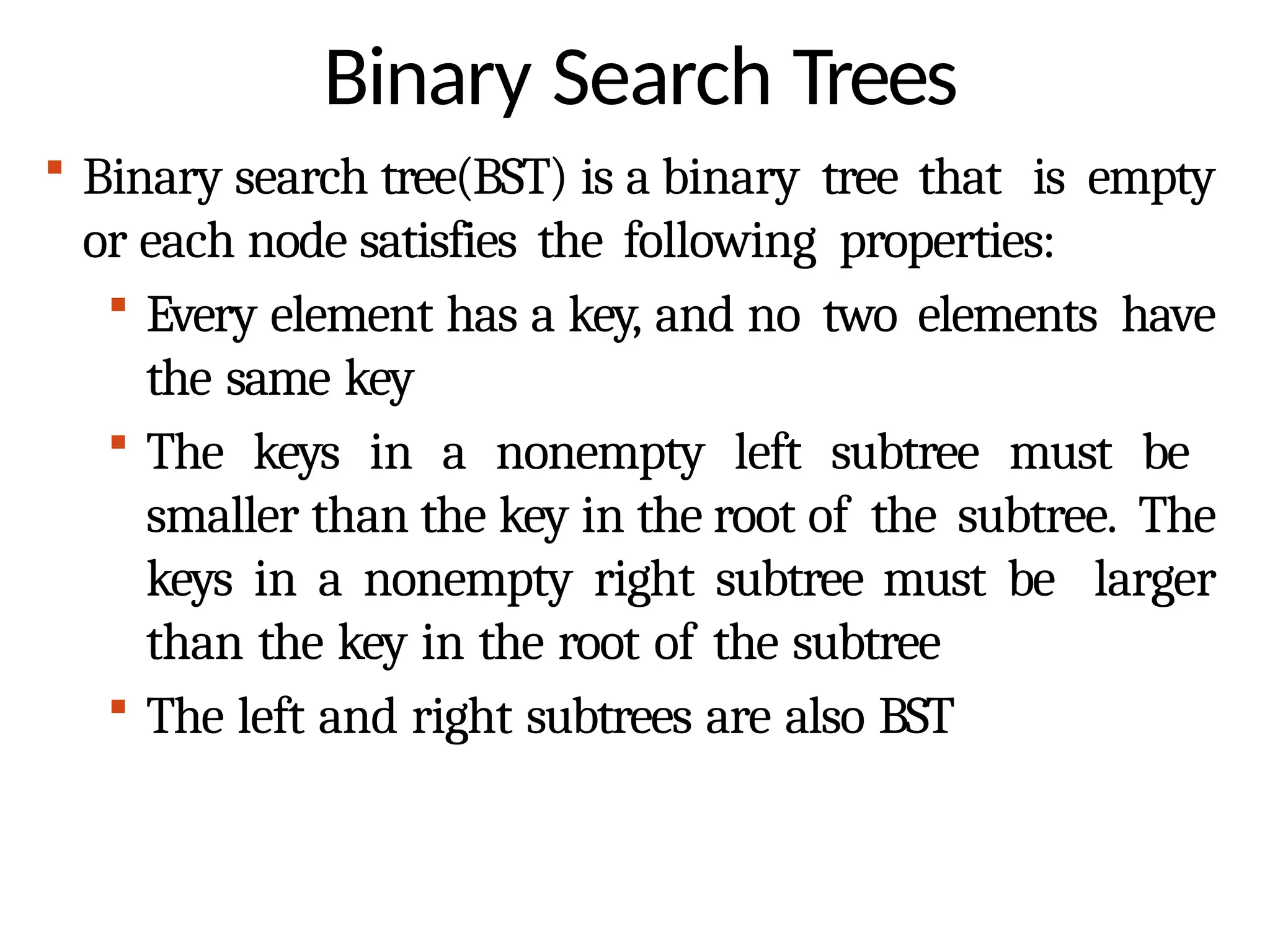
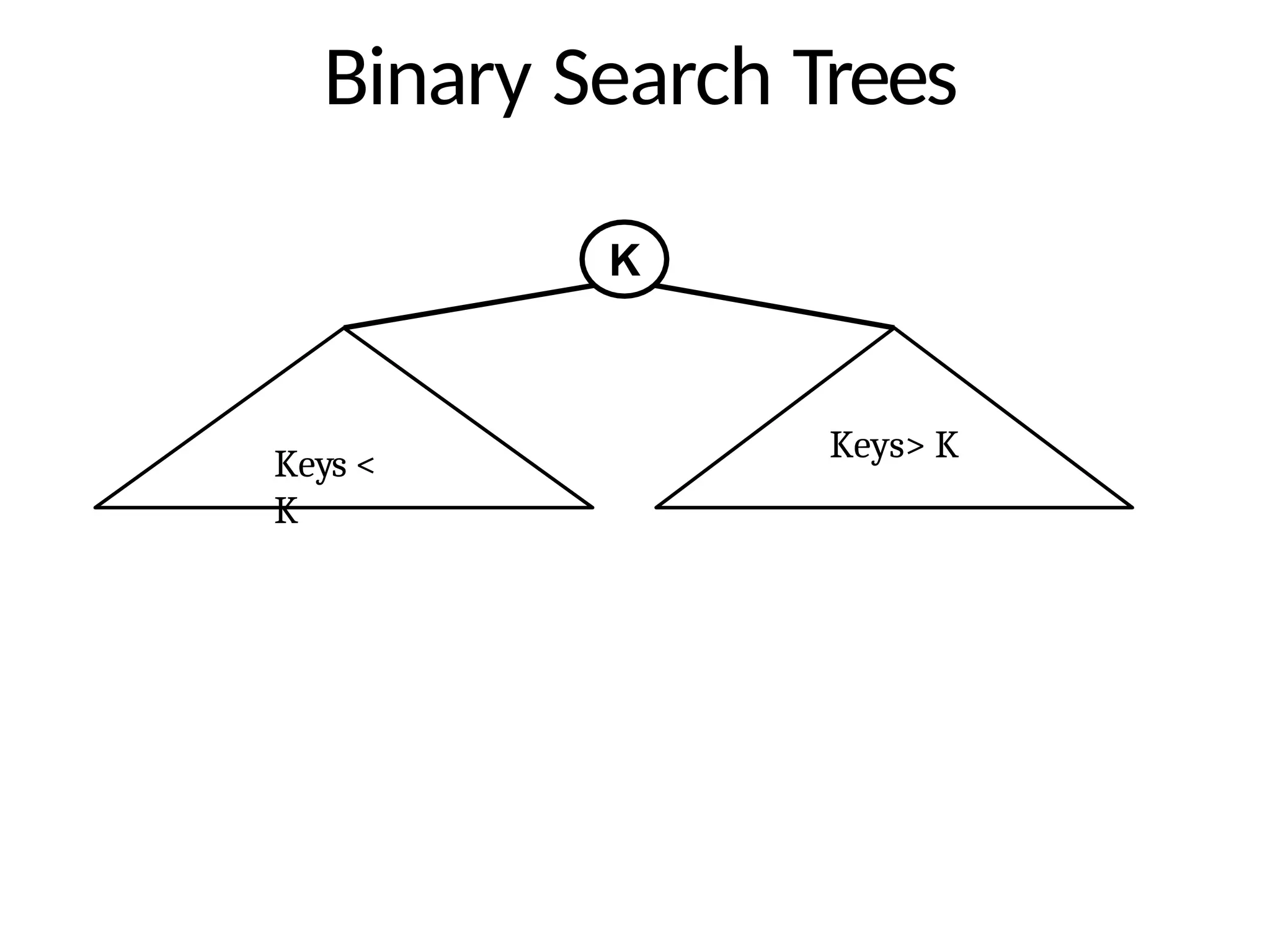
Binary Search Trees
Binary search tree(BST) is a binary tree that is empty
or each node satisfies the following properties:
Every element has a key, and no two elements have
the same key
The keys in a nonempty left subtree must be
smaller than the key in the root of the subtree. The
keys in a nonempty right subtree must be larger
than the key in the root of the subtree
The left and right subtrees are also BST
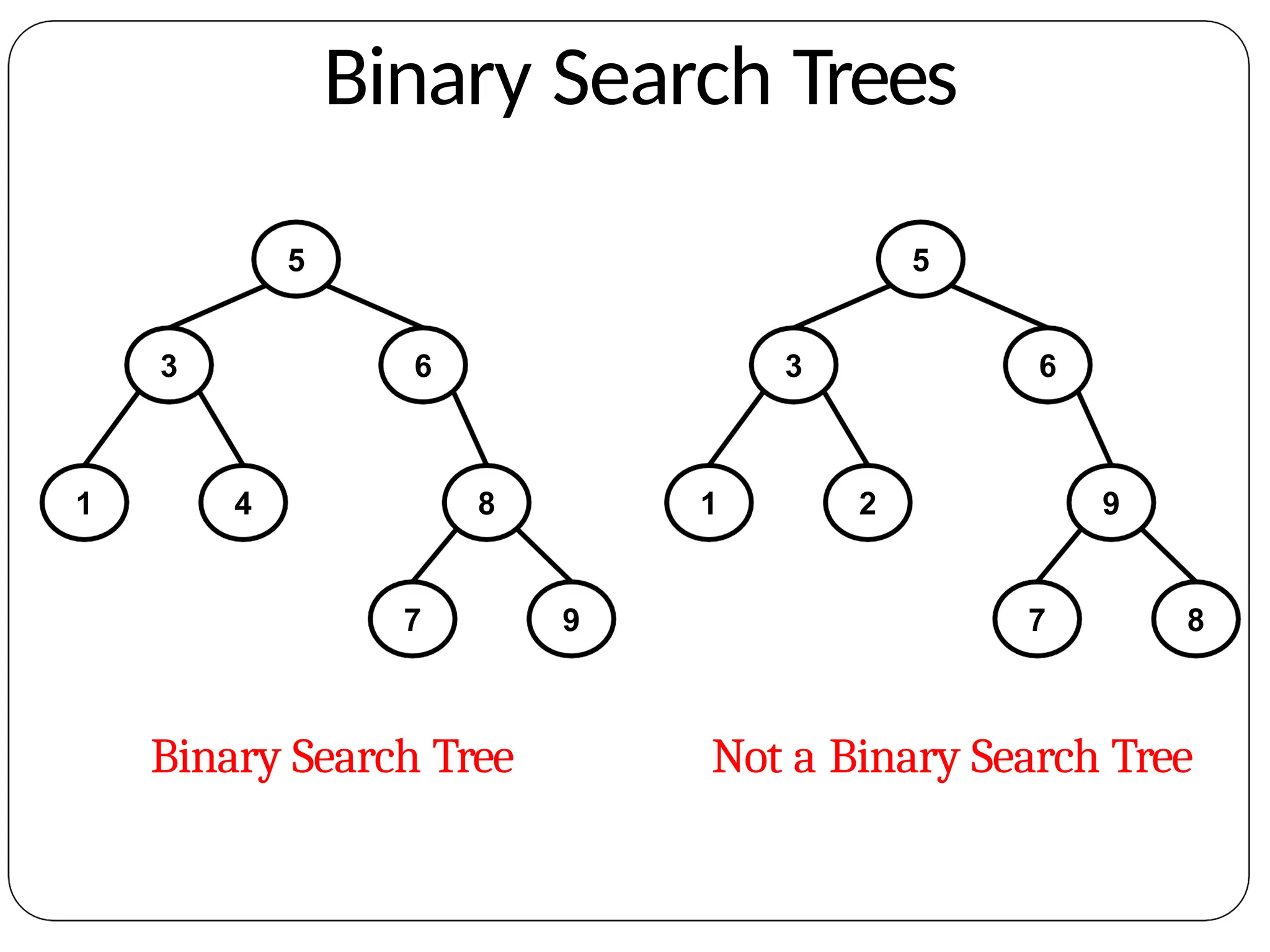
Binary Search Trees
5
36
1 4 8
7 9
5
3 6
1 2 9
7 8
Binary Search Tree Not a Binary Search Tree
128.
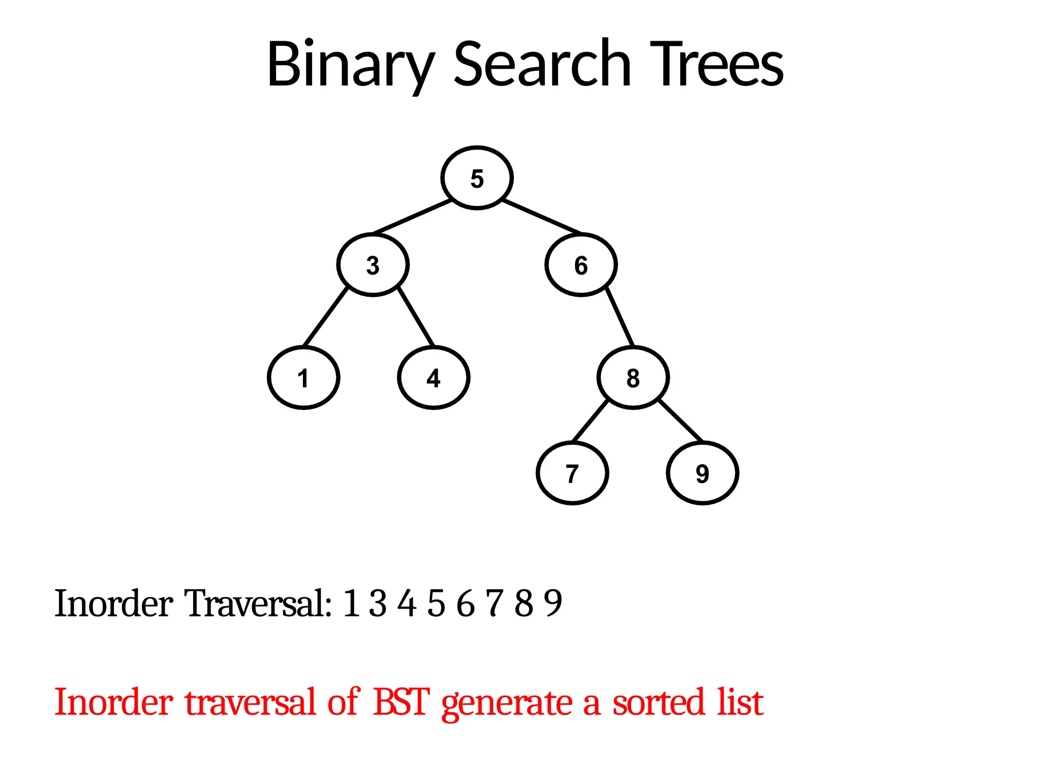
Binary Search Trees
5
36
1 4 8
7 9
Inorder Traversal: 1 3 4 5 6 7 8 9
Inorder traversal of BST generate a sorted list
129.
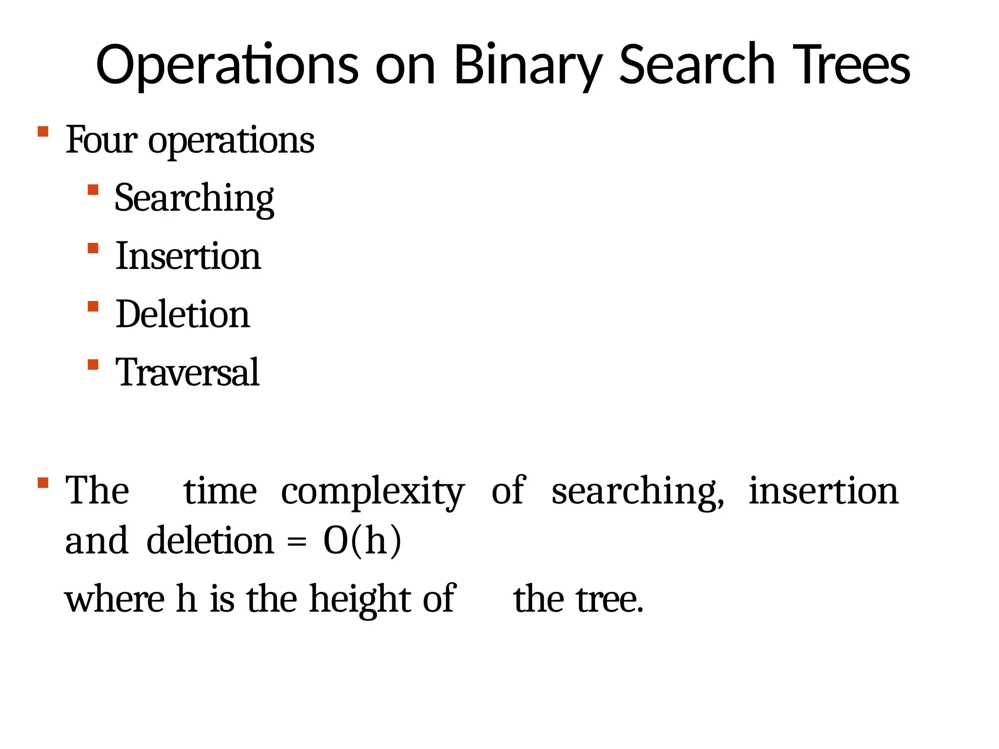
Operations on BinarySearch Trees
Four operations
Searching
Insertion
Deletion
Traversal
The time complexity of searching, insertion
and deletion = O(h)
where h is the height of the tree.
130.
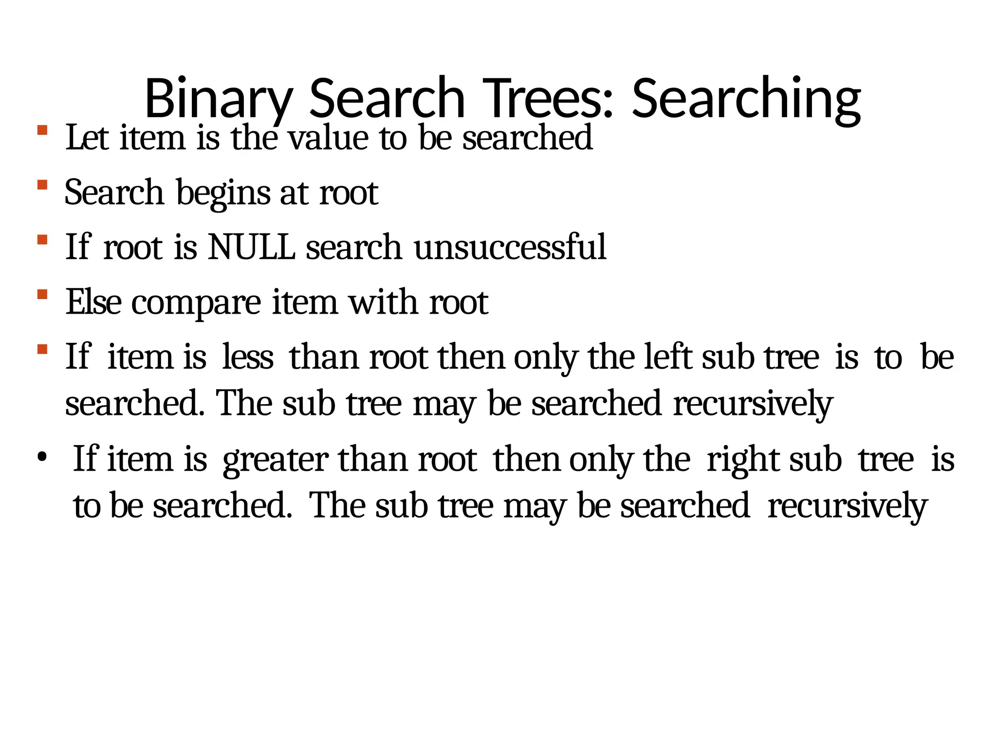
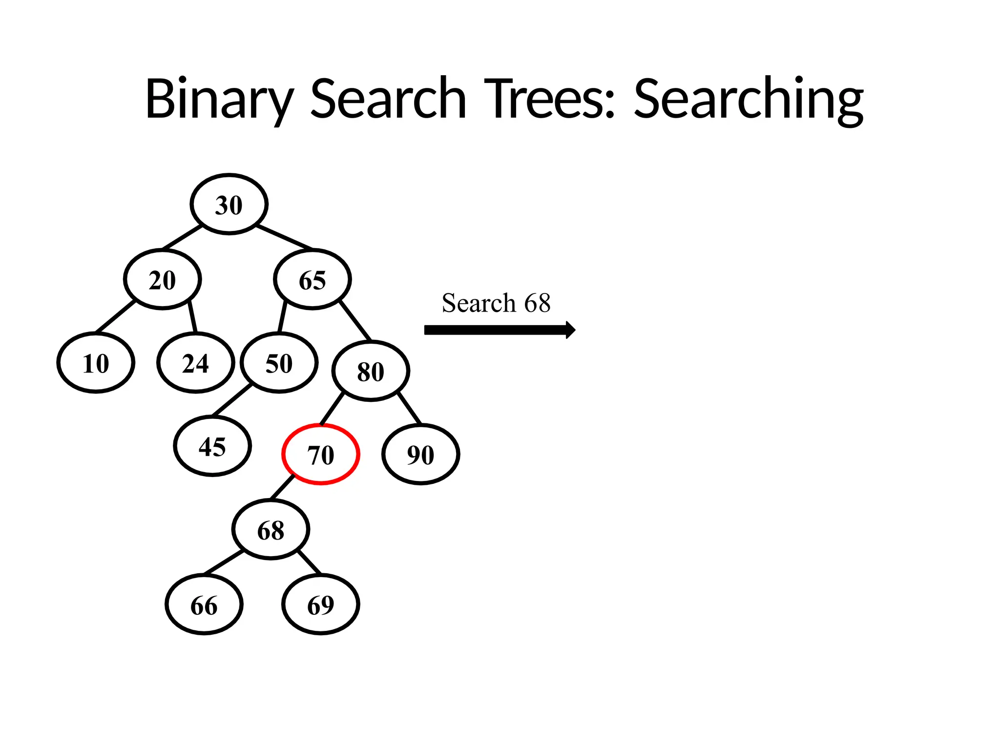
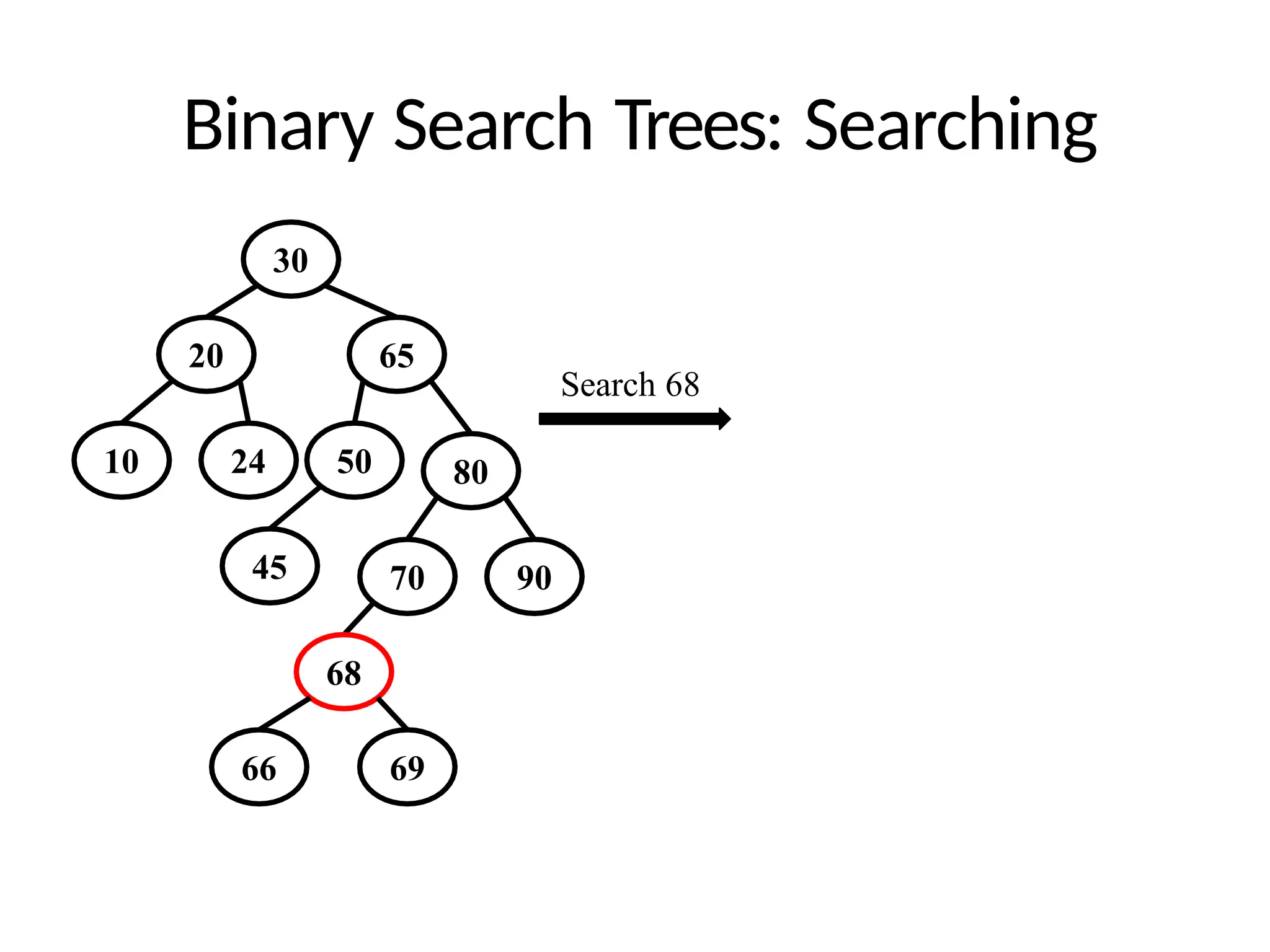
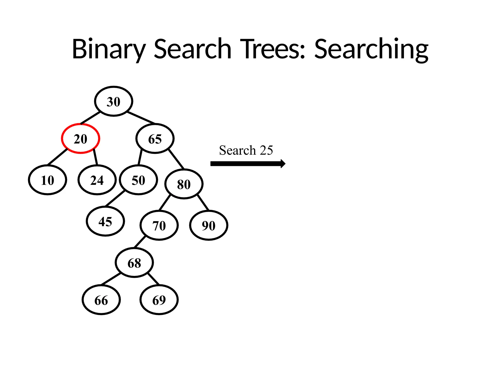
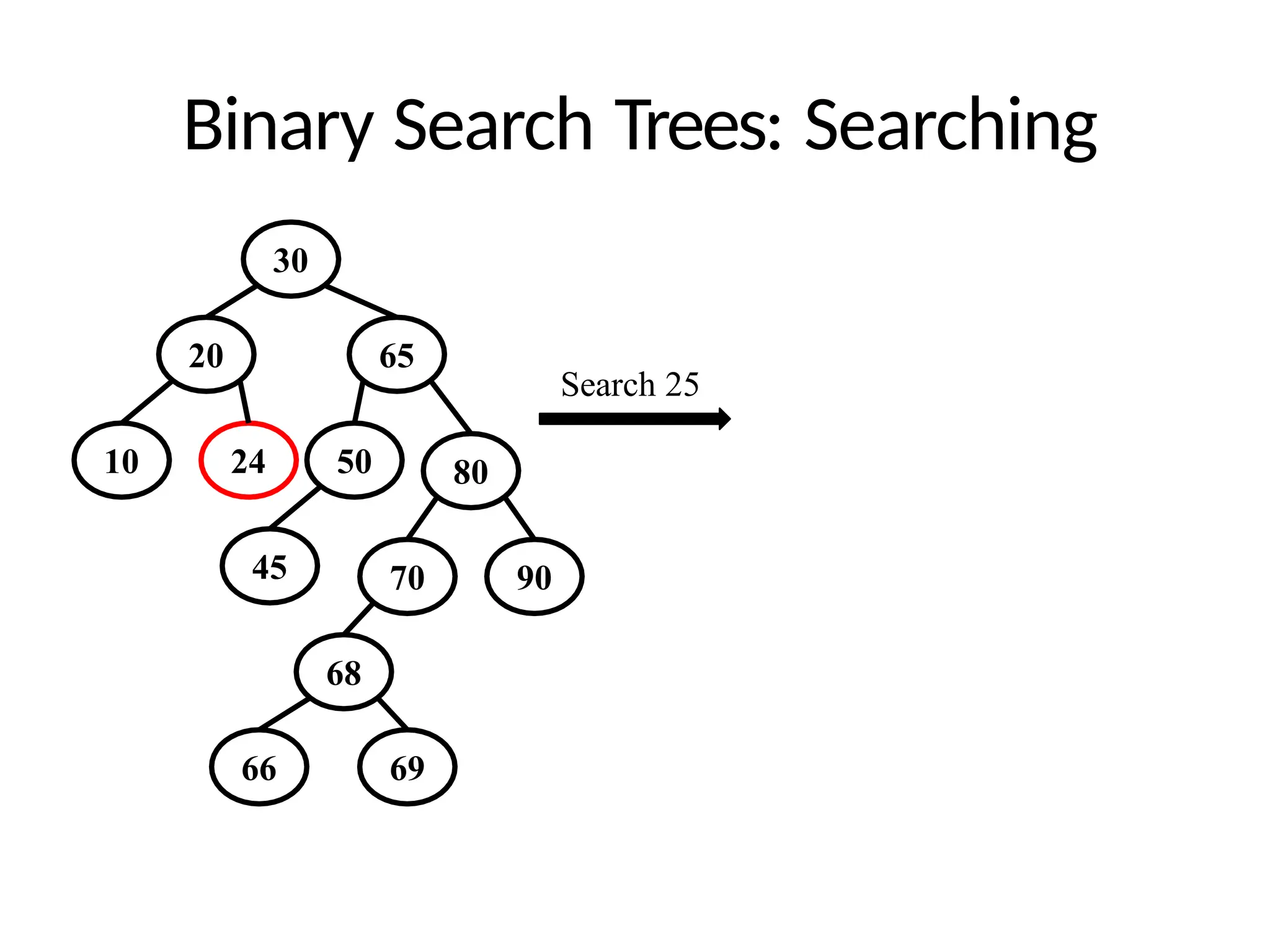
Binary Search Trees:Searching
Let item is the value to be searched
Search begins at root
If root is NULL search unsuccessful
Else compare item with root
If item is less than root then only the left sub tree is to be
searched. The sub tree may be searched recursively
• If item is greater than root then only the right sub tree is
to be searched. The sub tree may be searched recursively
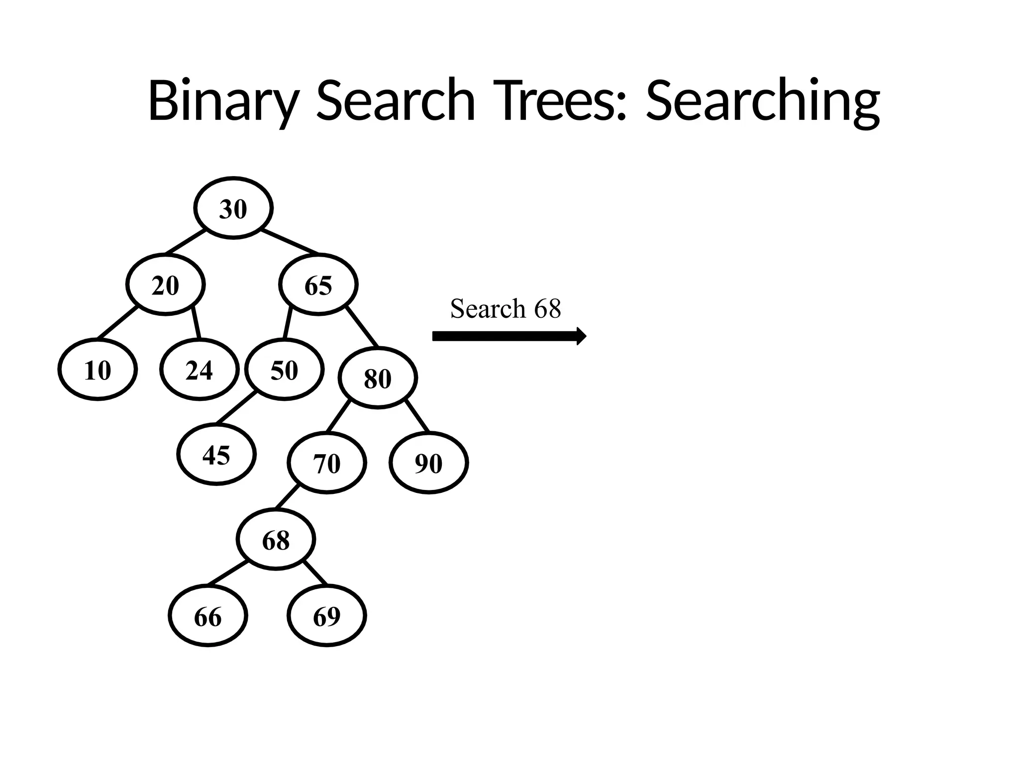
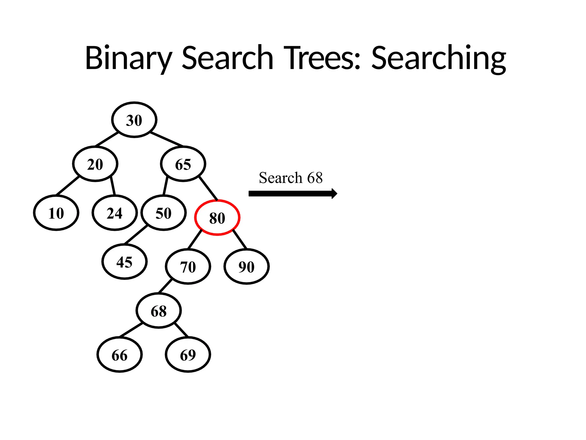
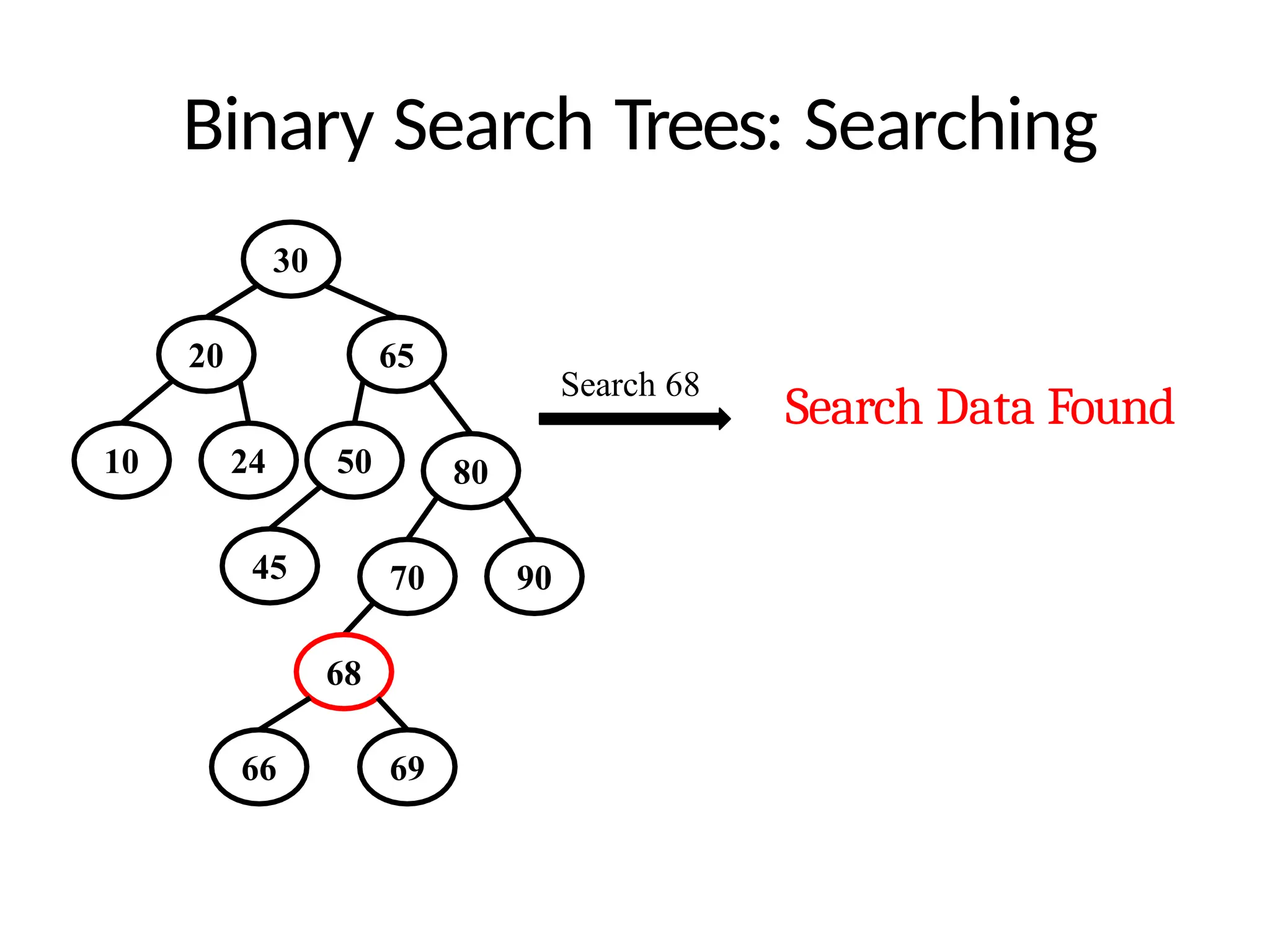
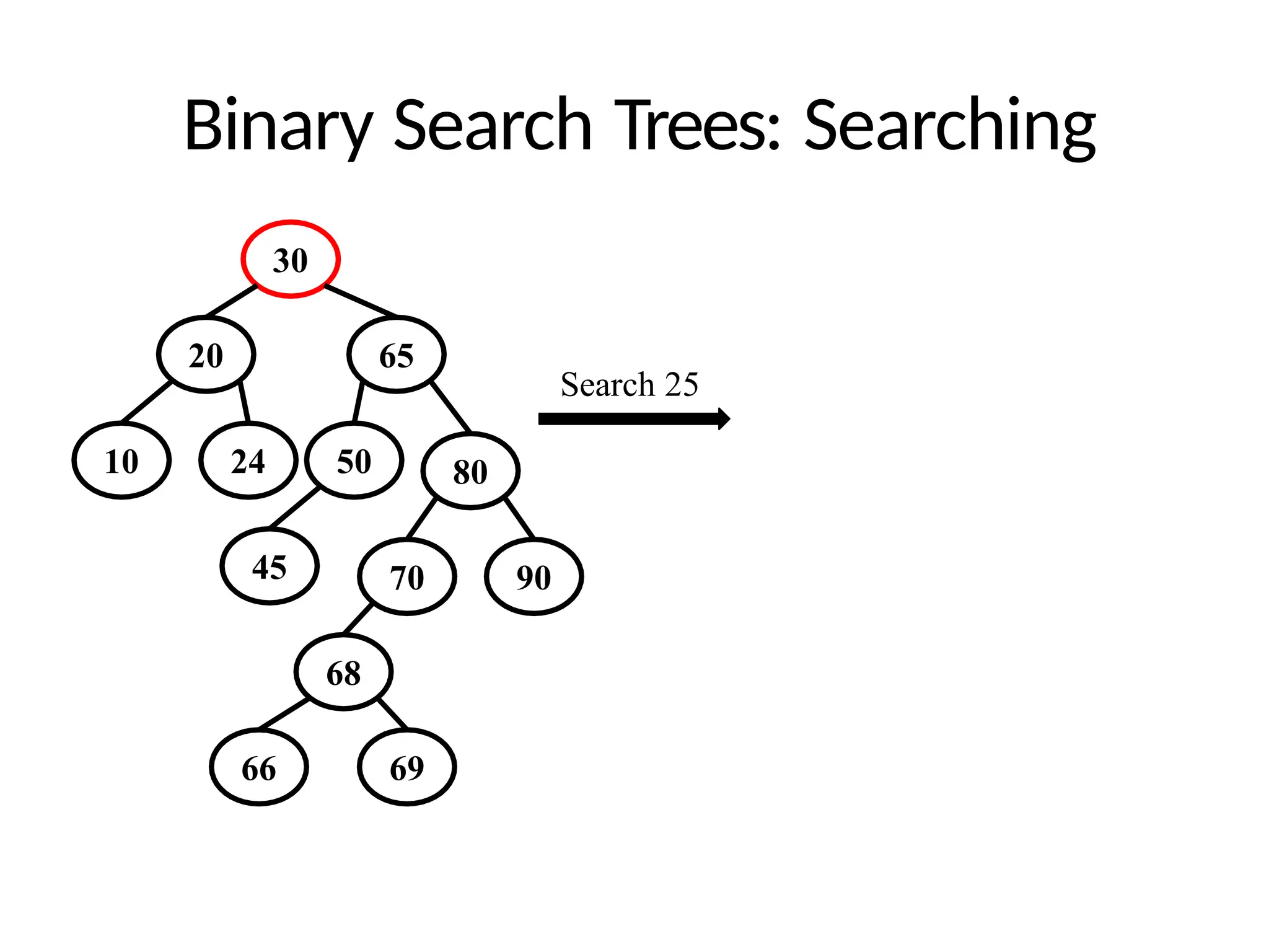
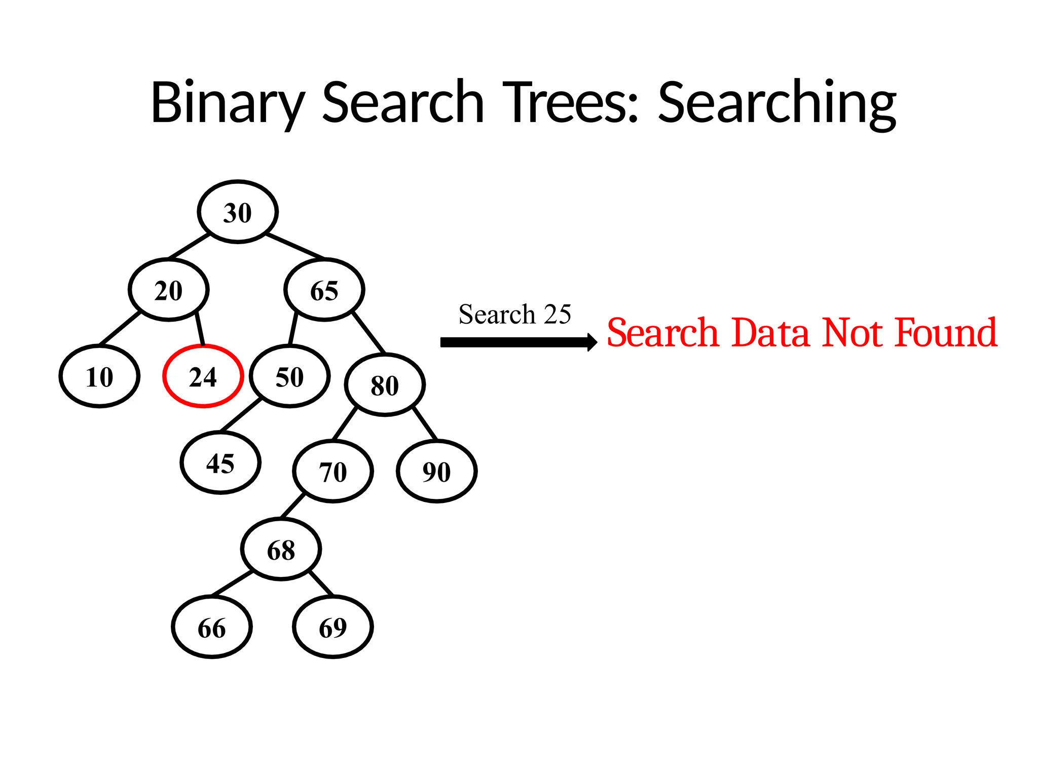
Binary Search Trees:Searching
30
20
10
65
80
24 50
45 70 90
68
Search 25
66 69
Search Data Not Found
143.
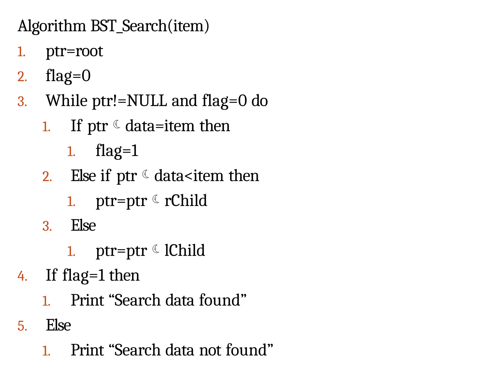
Algorithm BST_Search(item)
1. ptr=root
2.flag=0
3. While ptr!=NULL and flag=0 do
1. If ptrdata=item then
1. flag=1
2. Else if ptrdata<item then
1. ptr=ptrrChild
3. Else
1. ptr=ptrlChild
4. If flag=1 then
1. Print “Search data found”
5. Else
1. Print “Search data not found”
144.
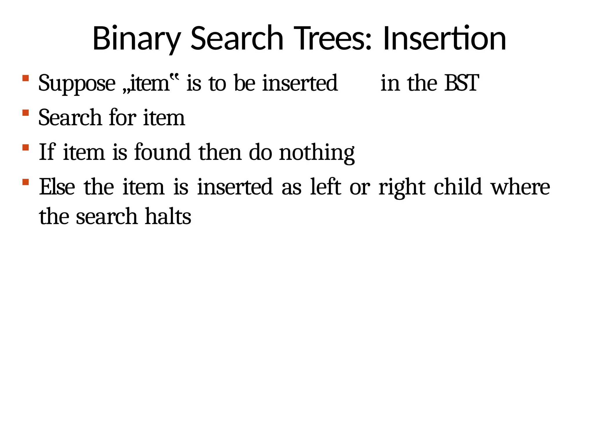
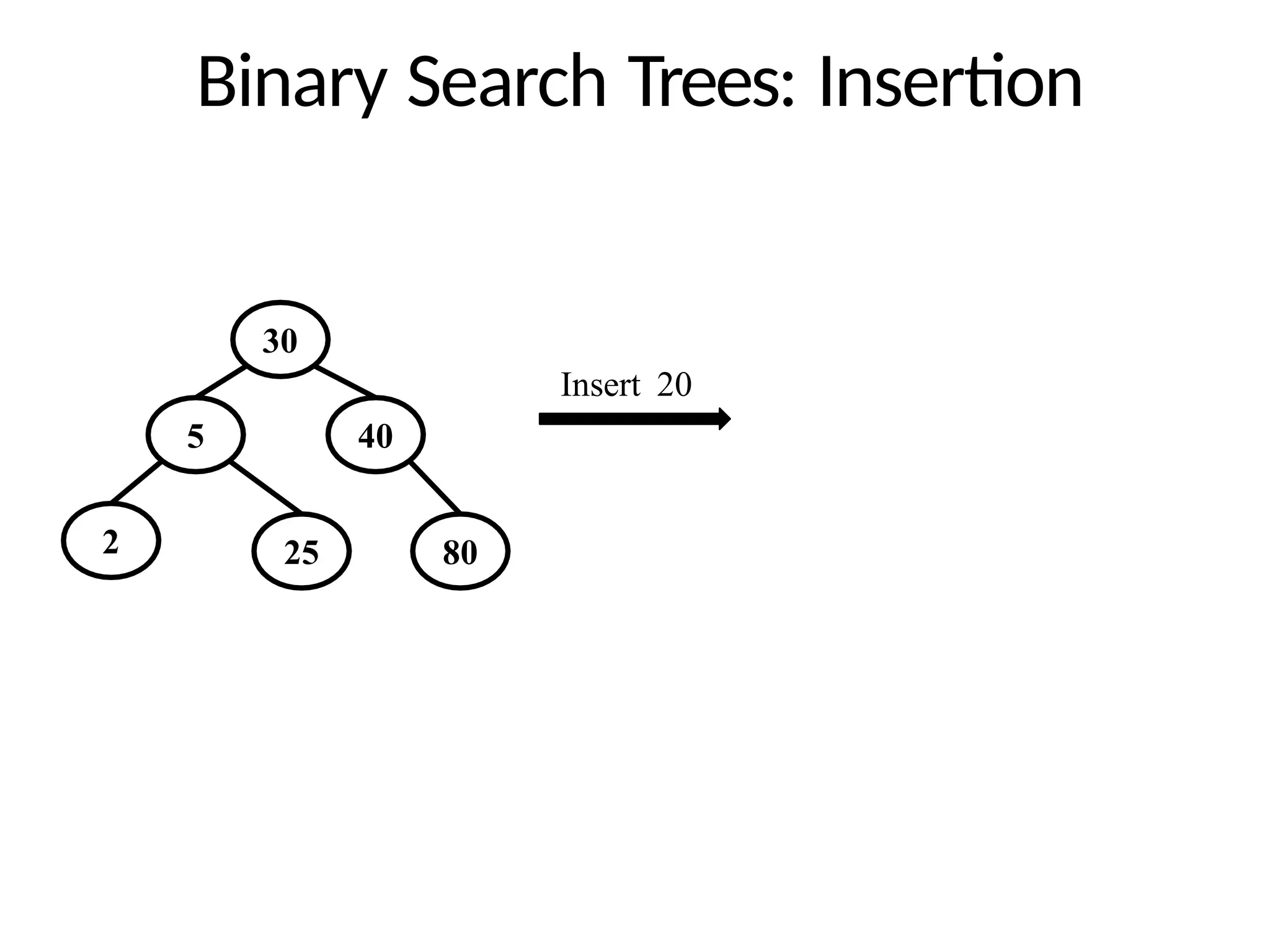
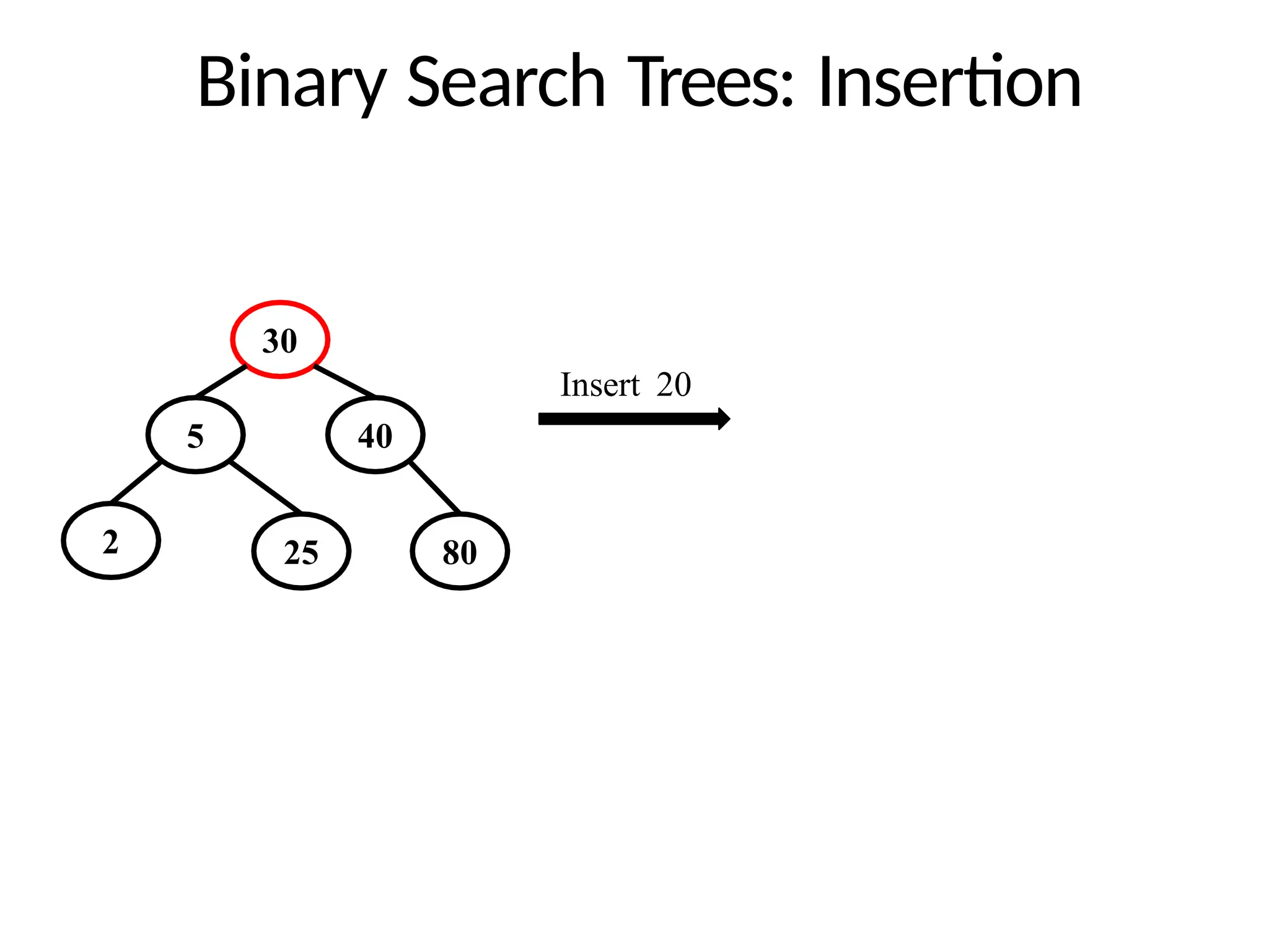
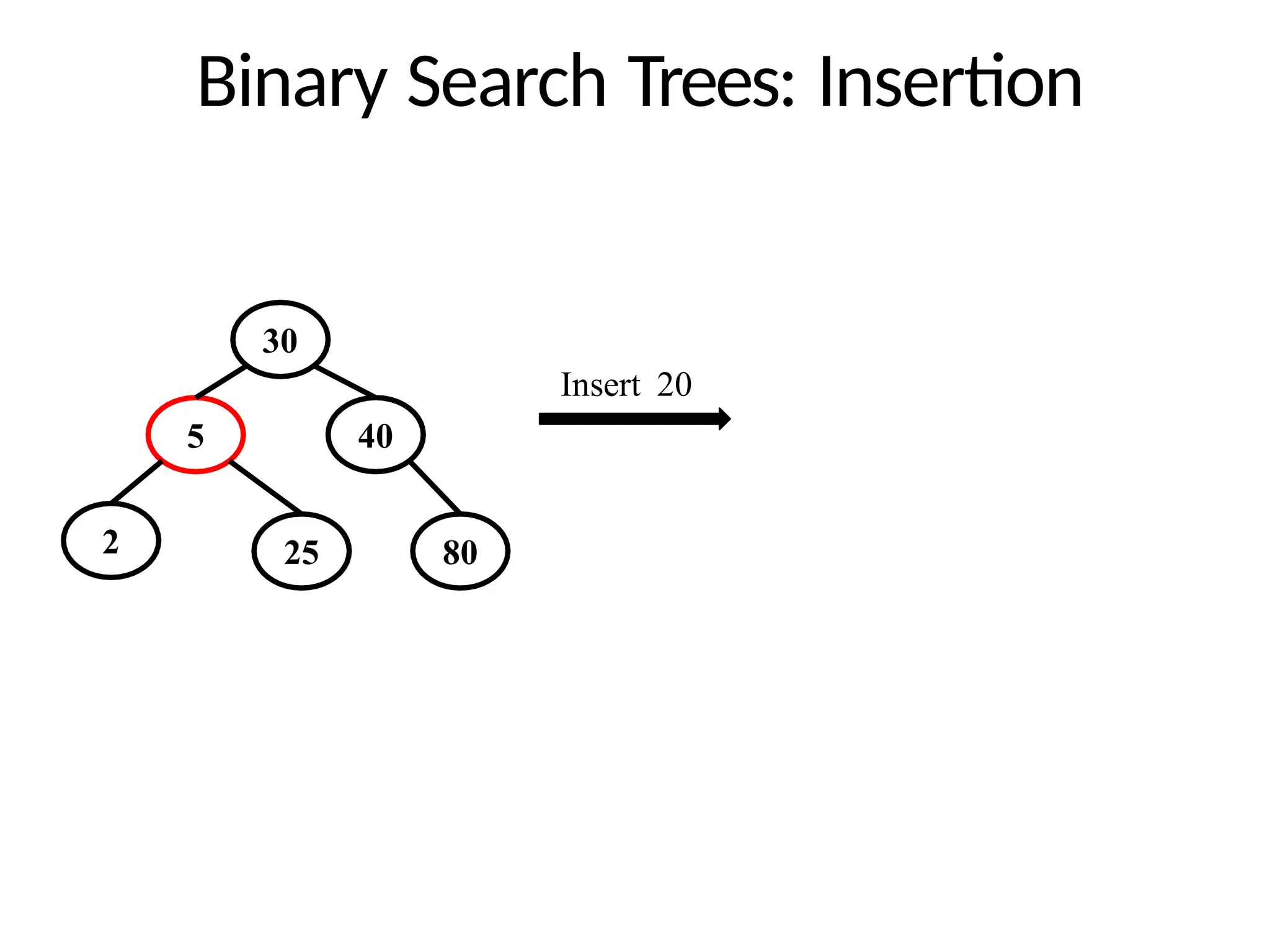
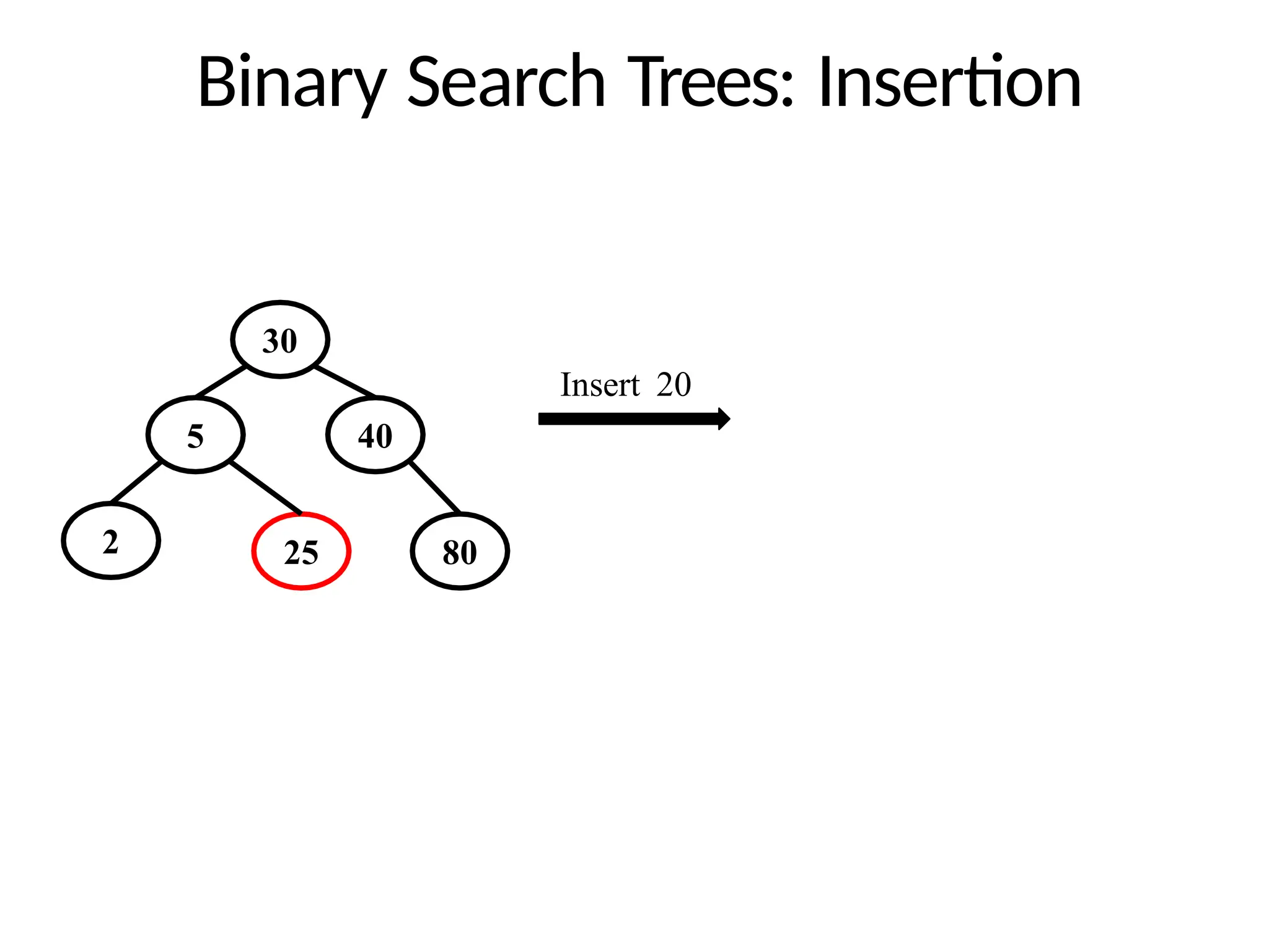
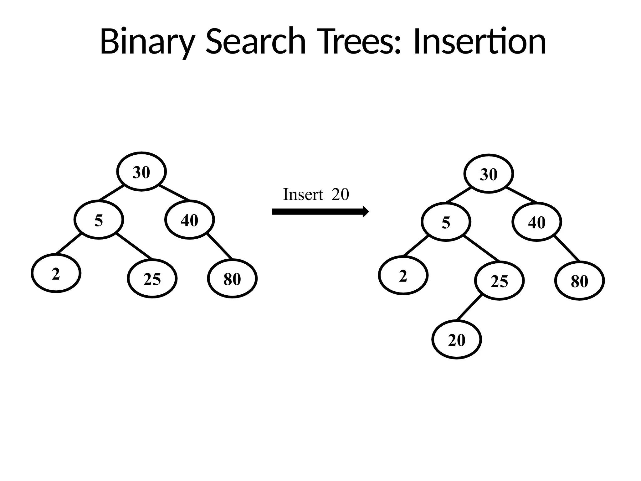
Binary Search Trees:Insertion
Suppose „item‟ is to be inserted in the BST
Search for item
If item is found then do nothing
Else the item is inserted as left or right child where
the search halts
145.
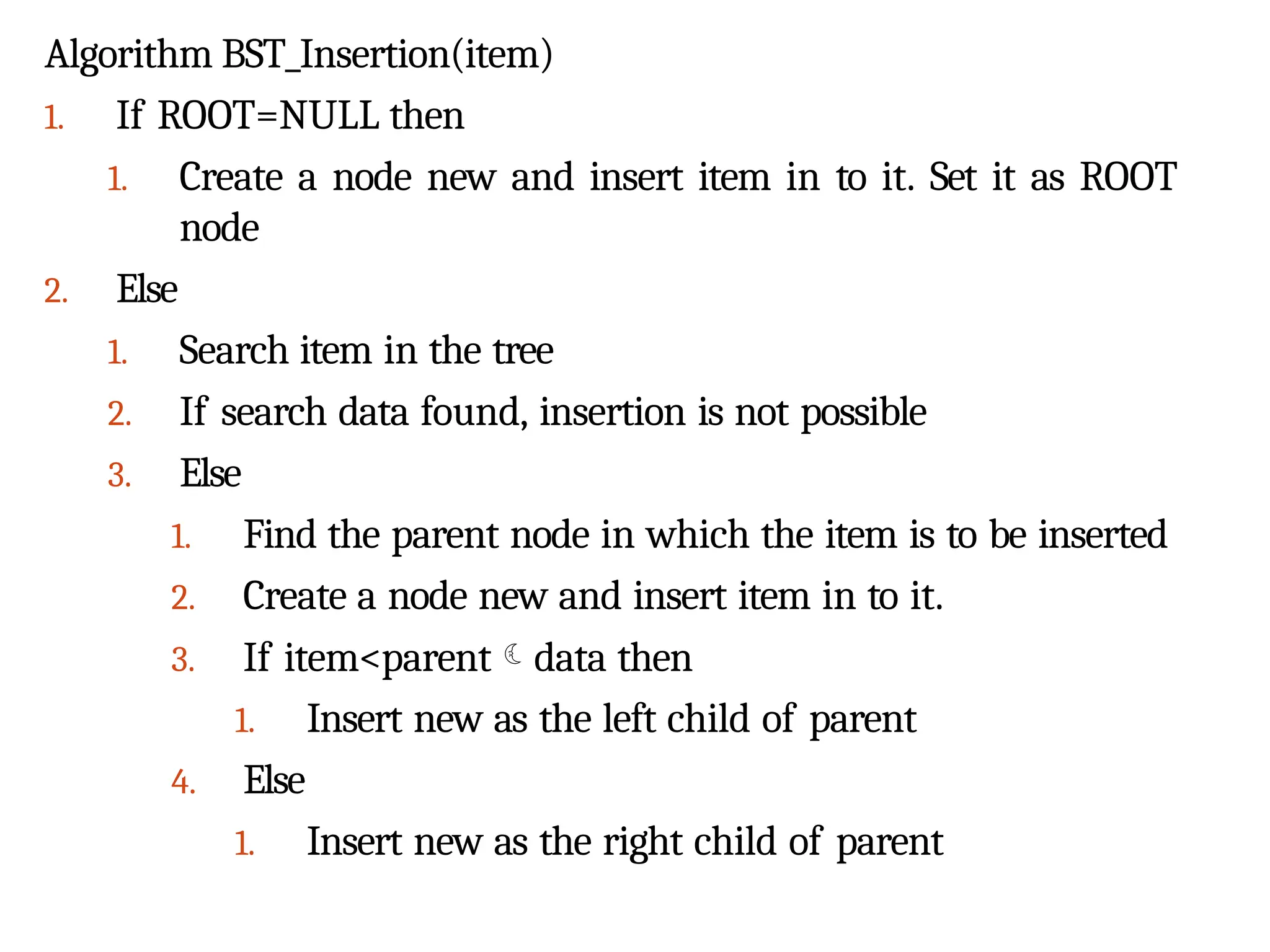
Algorithm BST_Insertion(item)
1. IfROOT=NULL then
1. Create a node new and insert item in to it. Set it as ROOT
node
2. Else
1. Search item in the tree
2. If search data found, insertion is not possible
3. Else
1. Find the parent node in which the item is to be inserted
2. Create a node new and insert item in to it.
3. If item<parentdata then
1. Insert new as the left child of parent
4. Else
1. Insert new as the right child of parent
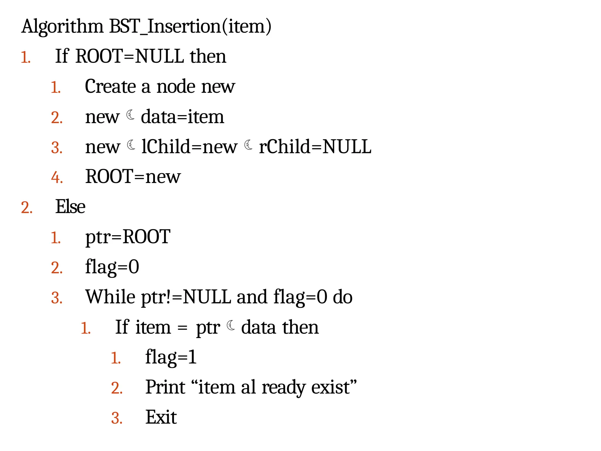
Algorithm BST_Insertion(item)
1. IfROOT=NULL then
1. Create a node new
2. newdata=item
3. newlChild=newrChild=NULL
4. ROOT=new
2. Else
1. ptr=ROOT
2. flag=0
3. While ptr!=NULL and flag=0 do
1. If item = ptrdata then
1. flag=1
2. Print “item al ready exist”
3. Exit
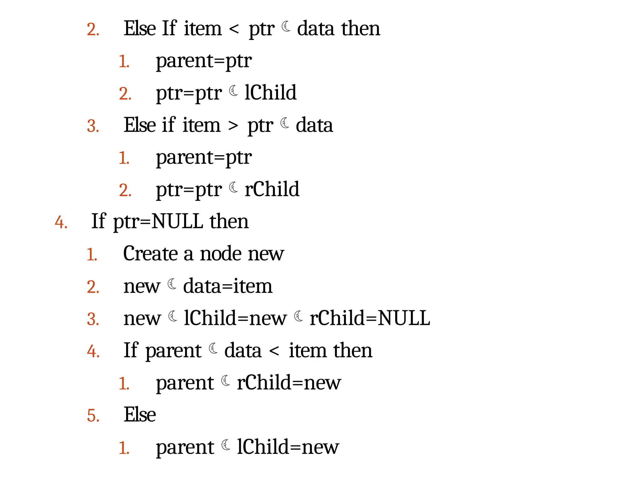
153.
2. Else Ifitem < ptrdata then
1. parent=ptr
2. ptr=ptrlChild
3. Else if item > ptrdata
1. parent=ptr
2. ptr=ptrrChild
4. If ptr=NULL then
1. Create a node new
2. newdata=item
3. newlChild=newrChild=NULL
4. If parentdata < item then
1. parentrChild=new
5. Else
1. parentlChild=new
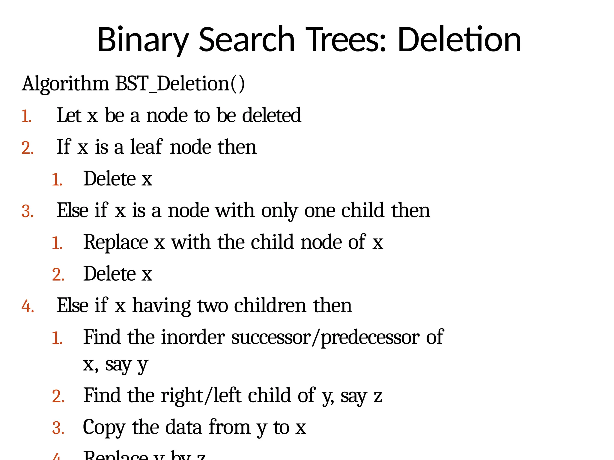
Binary Search Trees:Deletion
Algorithm BST_Deletion()
1. Let x be a node to be deleted
2. If x is a leaf node then
1. Delete x
3. Else if x is a node with only one child then
1. Replace x with the child node of x
2. Delete x
4. Else if x having two children then
1. Find the inorder successor/predecessor of
x, say y
2. Find the right/left child of y, say z
3. Copy the data from y to x
156.
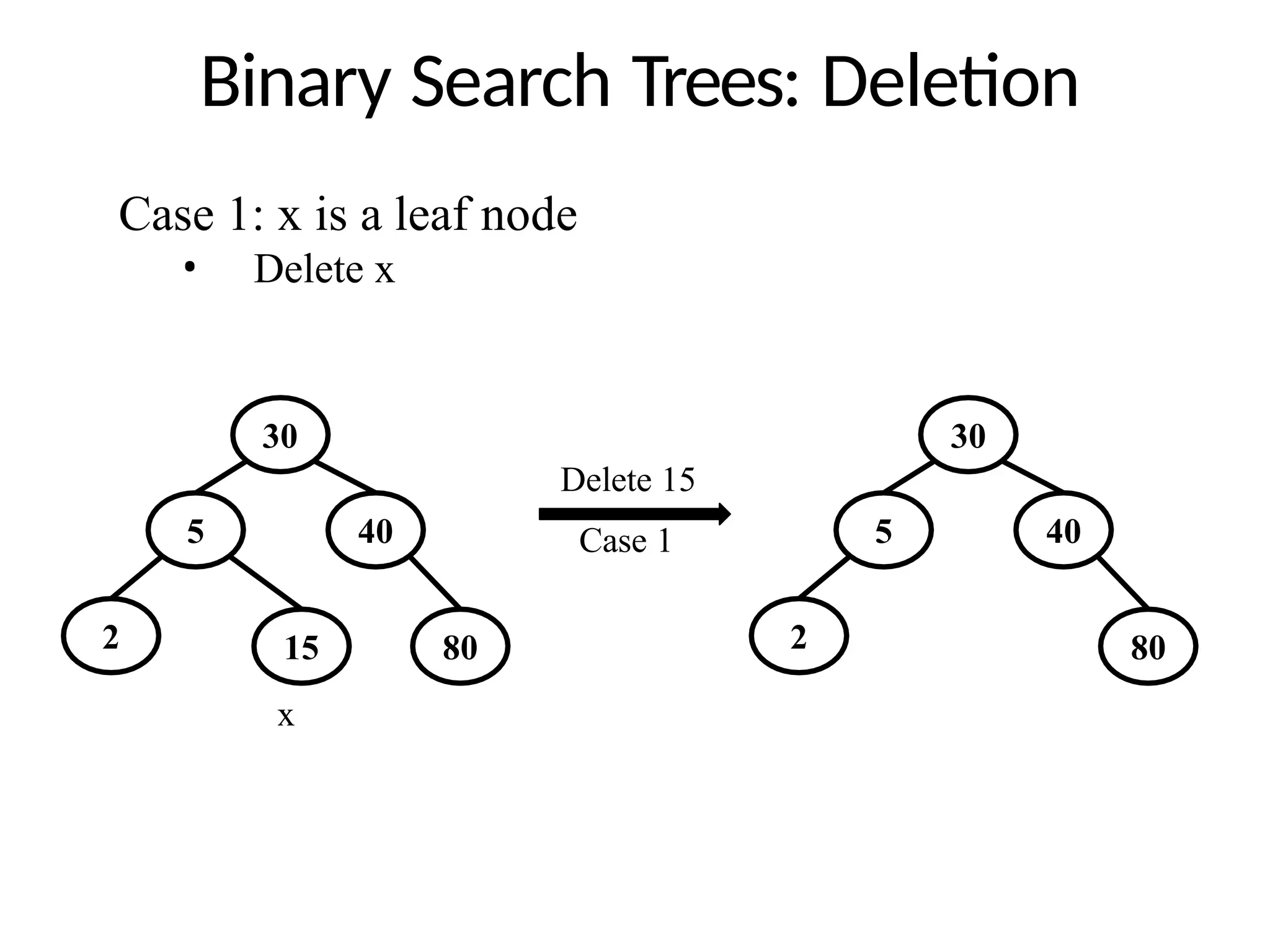
Binary Search Trees:Deletion
Case 1: x is a leaf node
• Delete x
30
5
2
40
80
30
5
2
40
80
15
x
Delete 15
Case 1
157.
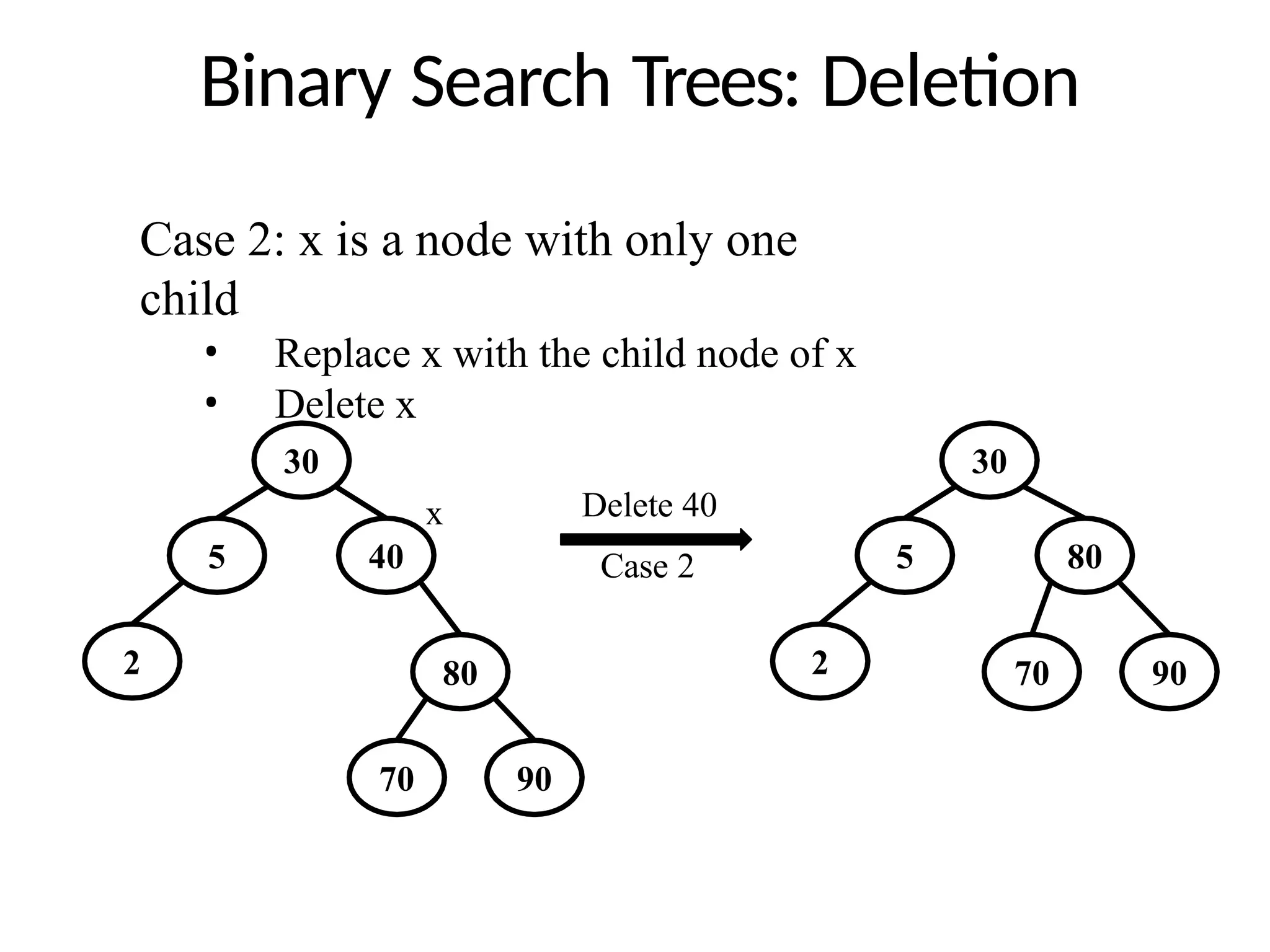
Binary Search Trees:Deletion
Case 2: x is a node with only one
child
• Replace x with the child node of x
• Delete x
30
5
2
40
80
30
5
2
80
x Delete 40
Case 2
70 90
70 90
158.
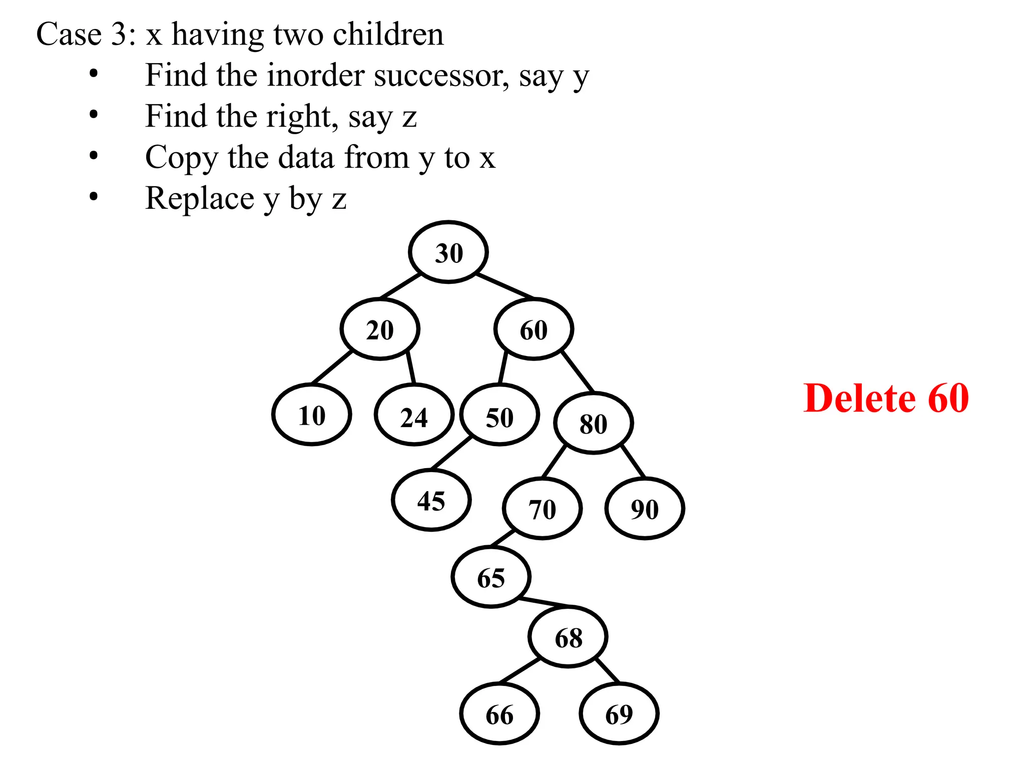
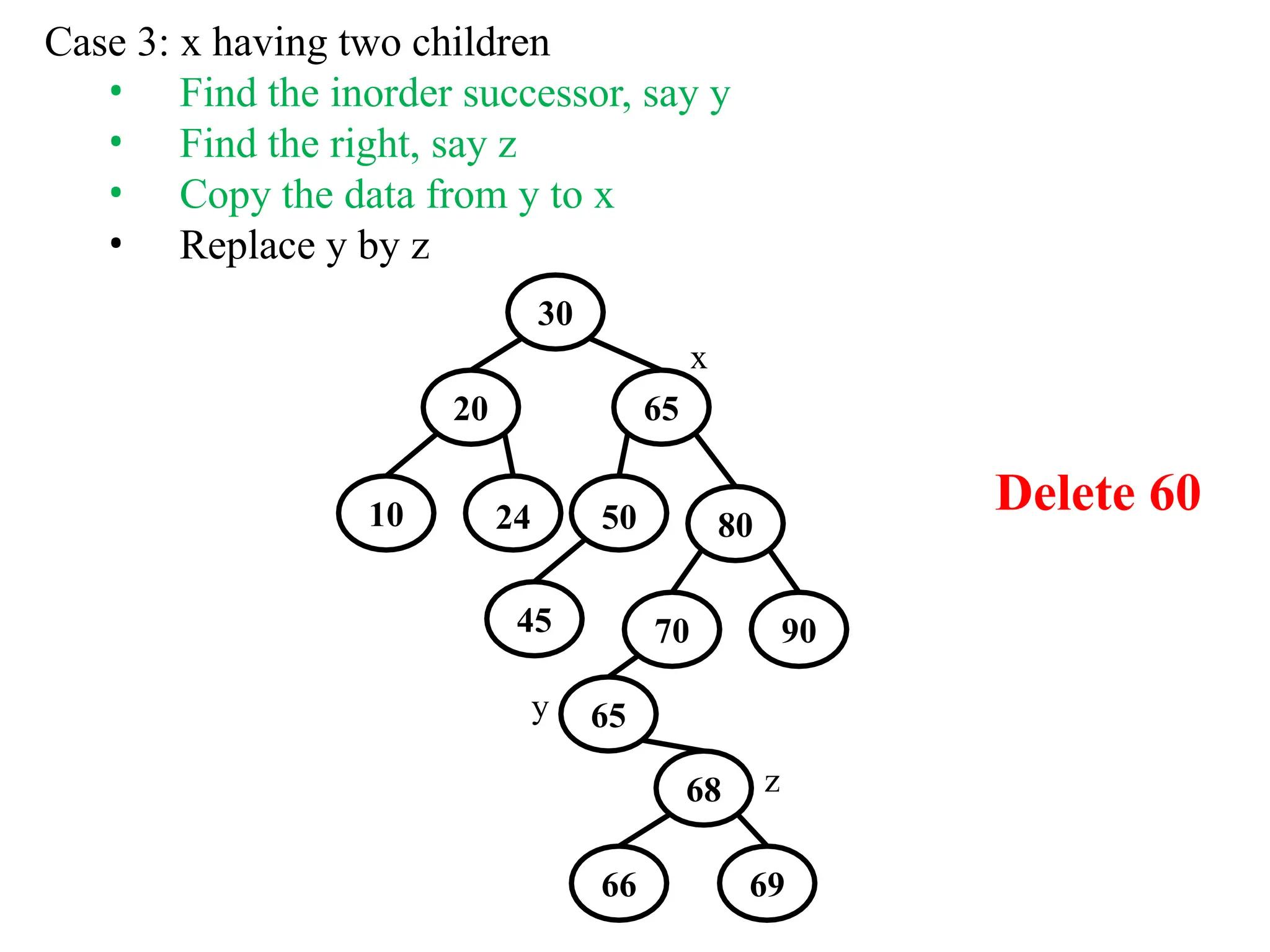
Case 3: xhaving two children
• Find the inorder successor, say y
• Find the right, say z
• Copy the data from y to x
• Replace y by z
30
10 80
20 60
24 50
45 70 90
65
68
Delete 60
66 69
159.
10 80
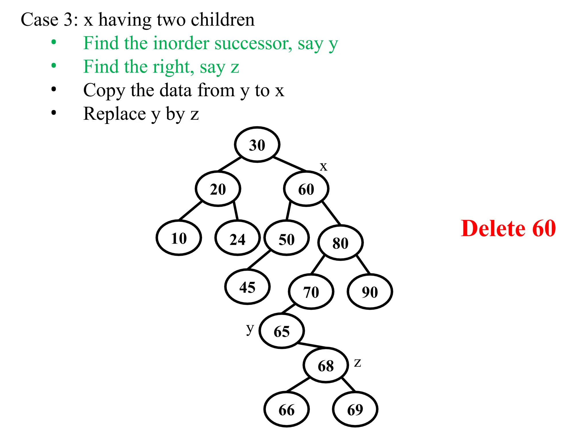
Delete 60
Case3: x having two children
• Find the inorder successor, say y
• Find the right, say z
• Copy the data from y to x
• Replace y by z
30
x
20 60
24 50
45 70 90
65
68
y
66 69
z
160.
10 80
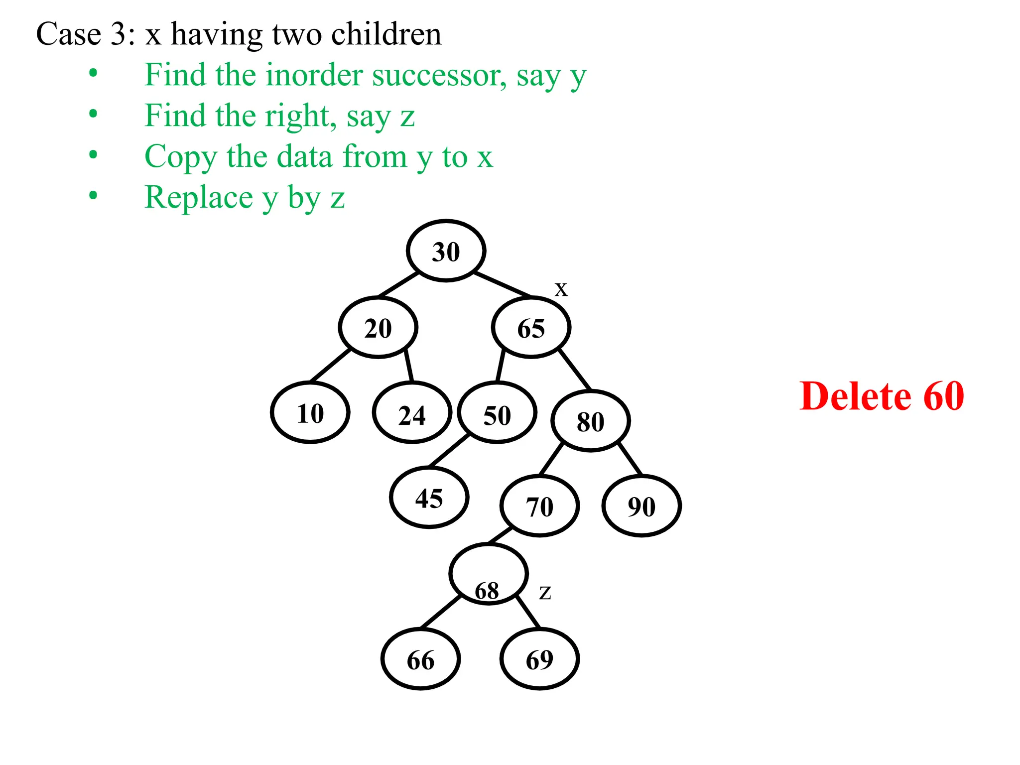
Case 3:x having two children
• Find the inorder successor, say y
• Find the right, say z
• Copy the data from y to x
• Replace y by z
30
x
20 65
24 50
45 70 90
65
68
y
66 69
z
Delete 60
161.
10 80
Case 3:x having two children
• Find the inorder successor, say y
• Find the right, say z
• Copy the data from y to x
• Replace y by z
30
x
20 65
24 50
45 70 90
66 69
68 z
Delete 60
162.
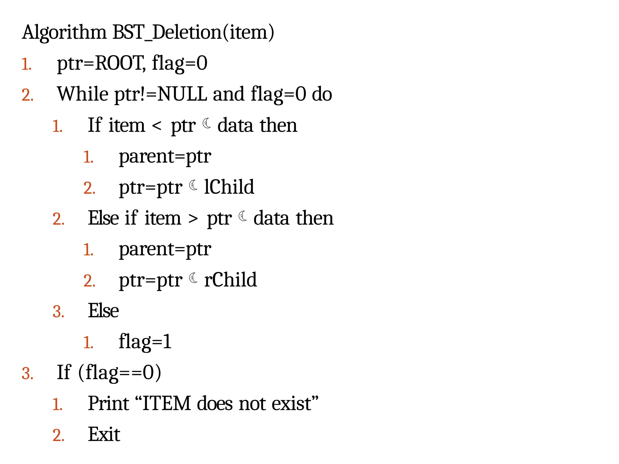
Algorithm BST_Deletion(item)
1. ptr=ROOT,flag=0
2. While ptr!=NULL and flag=0 do
1. If item < ptrdata then
1. parent=ptr
2. ptr=ptrlChild
2. Else if item > ptrdata then
1. parent=ptr
2. ptr=ptrrChild
3. Else
1. flag=1
3. If (flag==0)
1. Print “ITEM does not exist”
2. Exit
163.
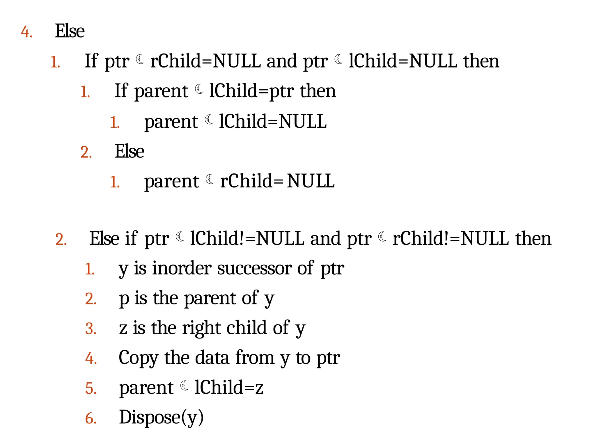
4. Else
1. IfptrrChild=NULL and ptrlChild=NULL then
1. If parentlChild=ptr then
1. parentlChild=NULL
2. Else
1. parentrChild=NULL
2. Else if ptrlChild!=NULL and ptrrChild!=NULL then
1. y is inorder successor of ptr
2. p is the parent of y
3. z is the right child of y
4. Copy the data from y to ptr
5. parentlChild=z
6. Dispose(y)
164.
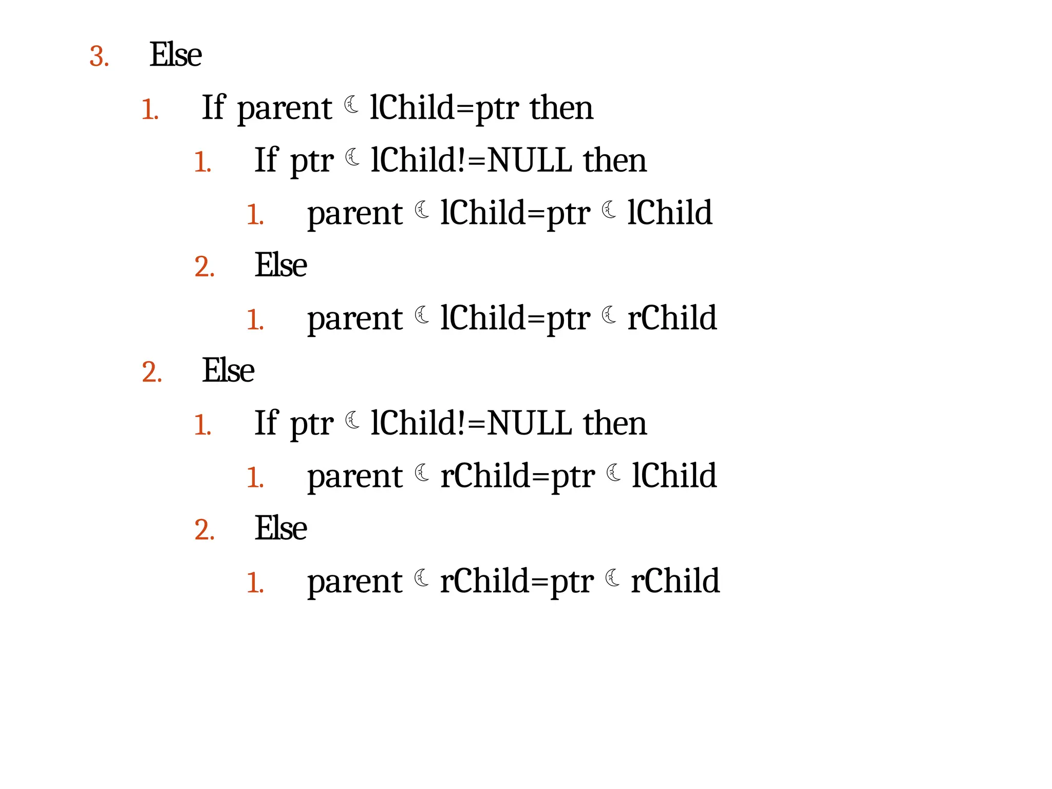
3. Else
1. IfparentlChild=ptr then
1. If ptrlChild!=NULL then
1. parentlChild=ptrlChild
2. Else
1. parentlChild=ptrrChild
2. Else
1. If ptrlChild!=NULL then
1. parentrChild=ptrlChild
2. Else
1. parentrChild=ptrrChild
165.
• A BSTis constructed by inserting the following
numbers in the order:
60,25,72,15,30,68,101,13,18,47,70,34. The
number of nodes in the left subtree is
________.
166.
Binary Search Trees:Applications
Remove duplicate values
Consider a collection of n data items A1,A2, …, AN.
Suppose we want to find and delete all duplicates
in the collection. Then, we can represent them as
BST and remove the duplicate values, while it
occurs.
Find the smallest data- Traverse the left subtree of BST
Find the largest data- Traverse the right subtree of BST
Find a particular data- Traverse the whole BST
167.
Height-balanced Binary
Search Trees
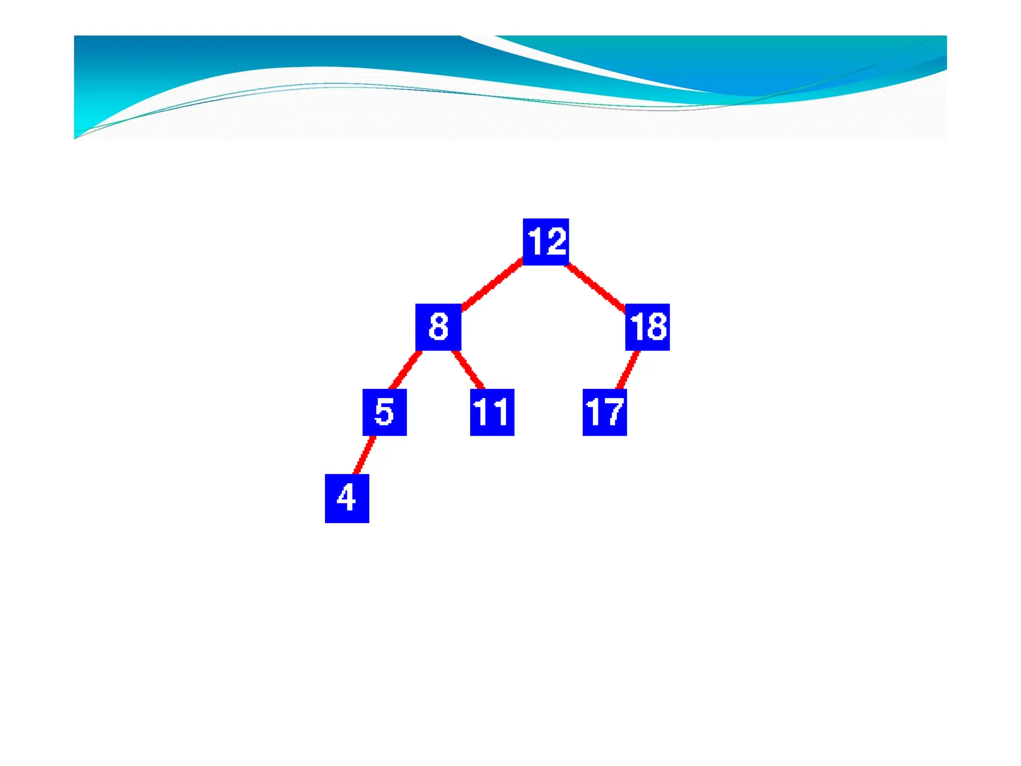
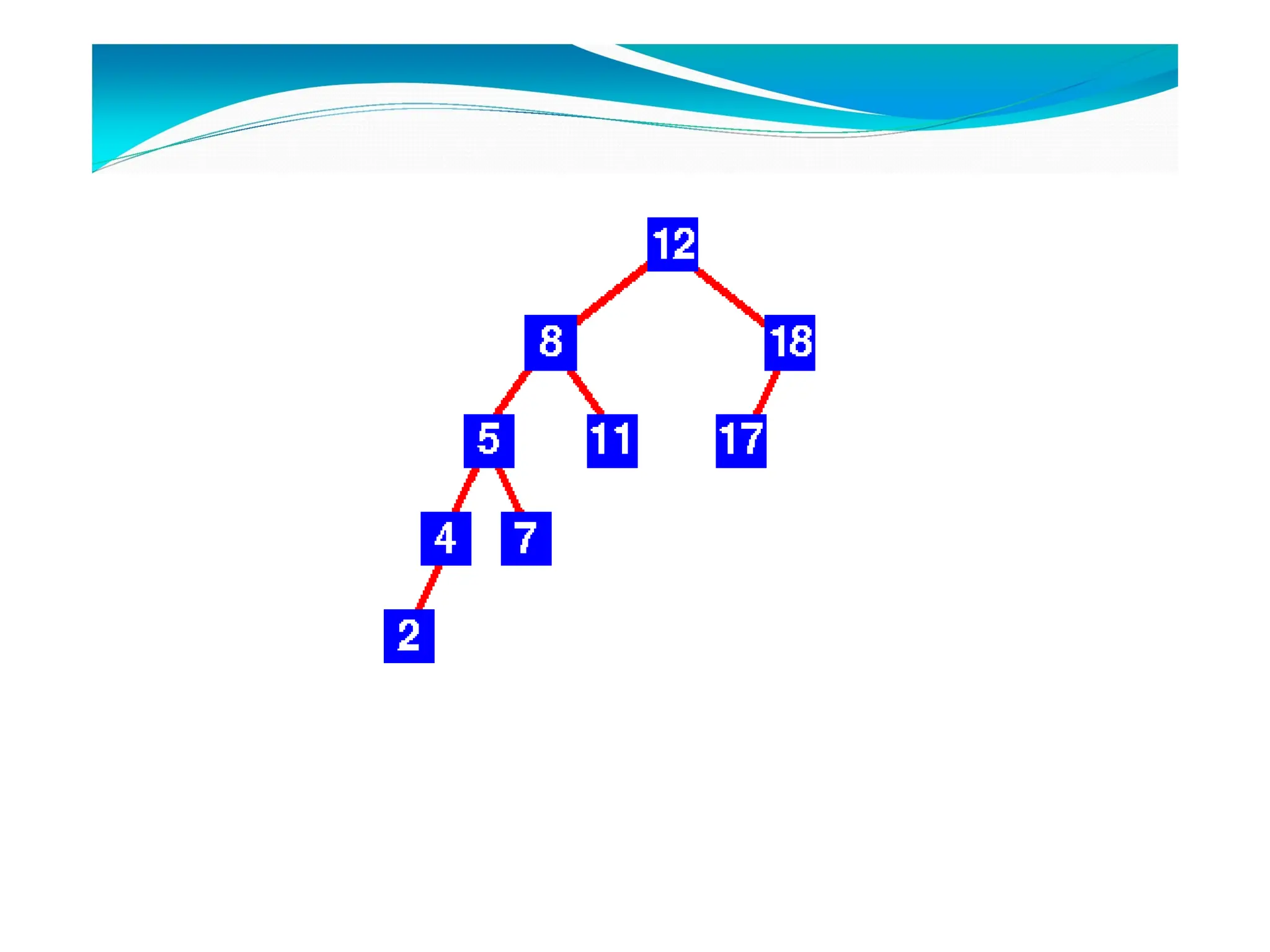
⚫Aself-balancing (or height-balanced) binary search
tree is any binary search tree that automatically keeps
its height (number of levels below the root) small after
arbitrary item insertions and deletions.
⚫A balanced tree is a BST whose every node above the
last level has non-empty left and right subtree.
⚫Number of nodes in a complete binary tree of height h is
2h+1 – 1. Hence, a binary tree of n elements is balanced
if:
2h – 1 < n <= 2h+1 - 1
168.
AVL
Trees
⚫Named after RussianMathematicians: G.M. Adelson-
Velskii and E.M. Landis who discovered them in 1962.
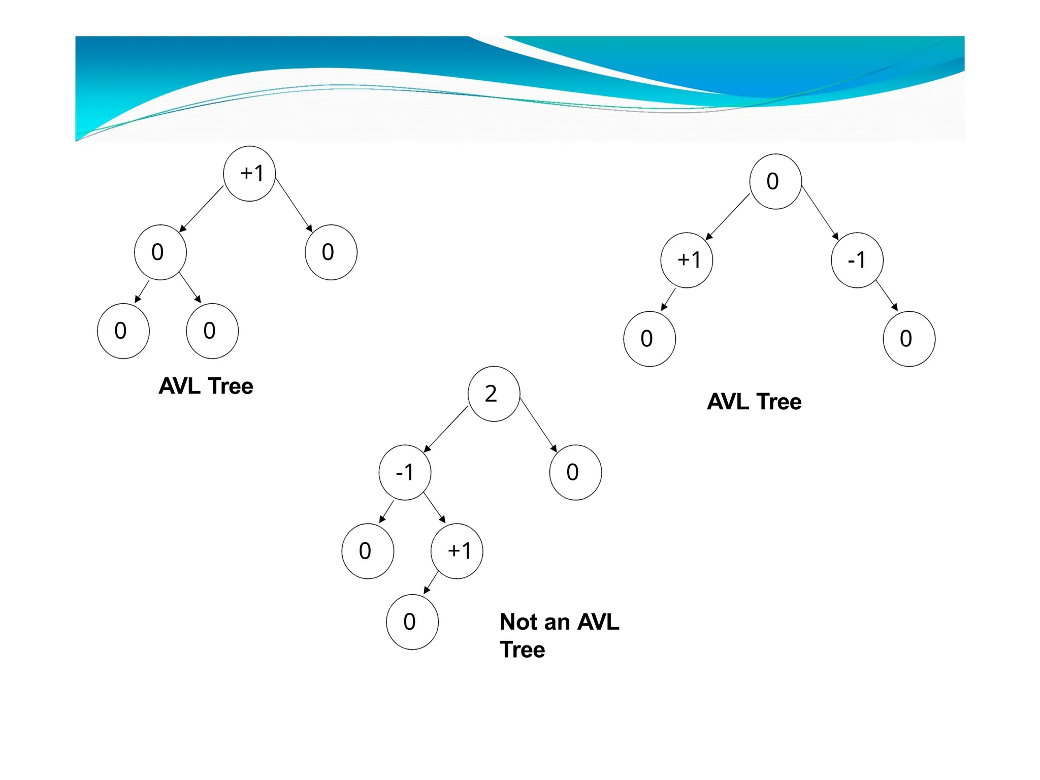
⚫An AVL tree is a binary search tree which has the
following properties:
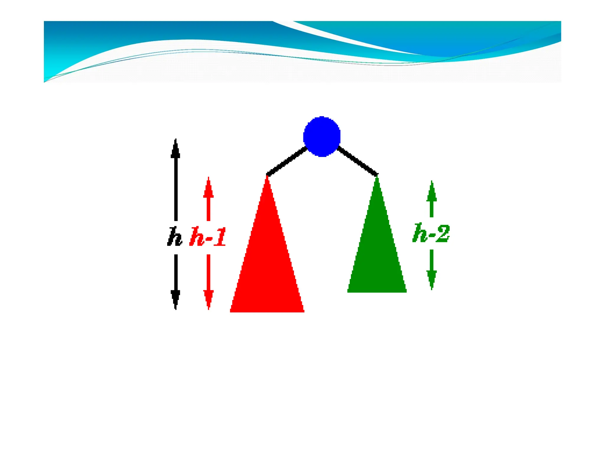
⚫The sub-trees of every node differ in height by at most
one.
⚫Every sub-tree is an AVL tree.
170.
⚫Implementations of AVLtree insertion rely on adding
an extra attribute, the balance factor to each node.
⚫ Balance factor (bf) = HL - HR
⚫An empty binary tree is an AVL tree.
⚫A non-empty binary tree T is an AVL tree iff :
⚫ | HL - HR | <= 1
⚫For an AVL tree, the balance factor, HL - HR , of a node can
be either 0, 1 or -1.
171.
⚫The balance factorindicates whether the tree is:
⚫left-heavy (the height of the left sub-tree is 1 greater than
the right sub-tree),
⚫balanced (both sub-trees are of the same height) or
⚫right-heavy (the height of the right sub-tree is 1 greater
than the left sub-tree).
⚫Insertion is similarto that of a BST.
⚫After inserting a node, it is necessary to check each of
the node's ancestors for consistency with the rules of
AVL.
⚫If after inserting an element, the balance of any tree is
destroyed then a rotation is performed to restore the
balance.
AVL Tree
Insertion
176.
⚫For each nodechecked, if the balance factor remains
−1, 0, or +1 then no rotations are necessary.
⚫However, if balance factor becomes less than -1 or
greater than +1, the subtree rooted at this node is
unbalanced.
177.
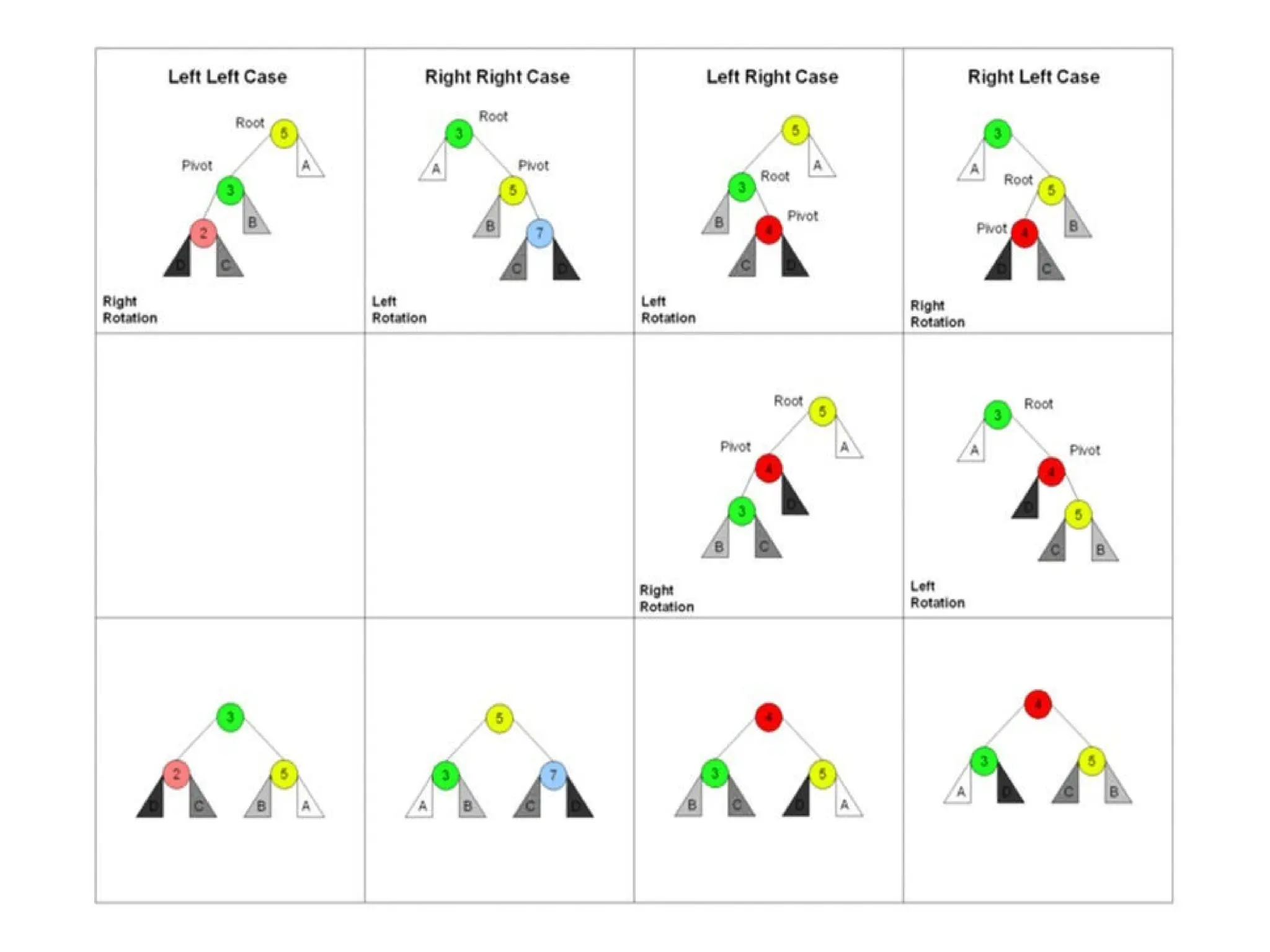
⚫Theorem: When anAVL tree becomes unbalanced after
an insertion, exactly one single or double rotation is
required to balance the tree.
⚫Let A be the root of the unbalanced subtree.
⚫There are four cases which need to be considered.
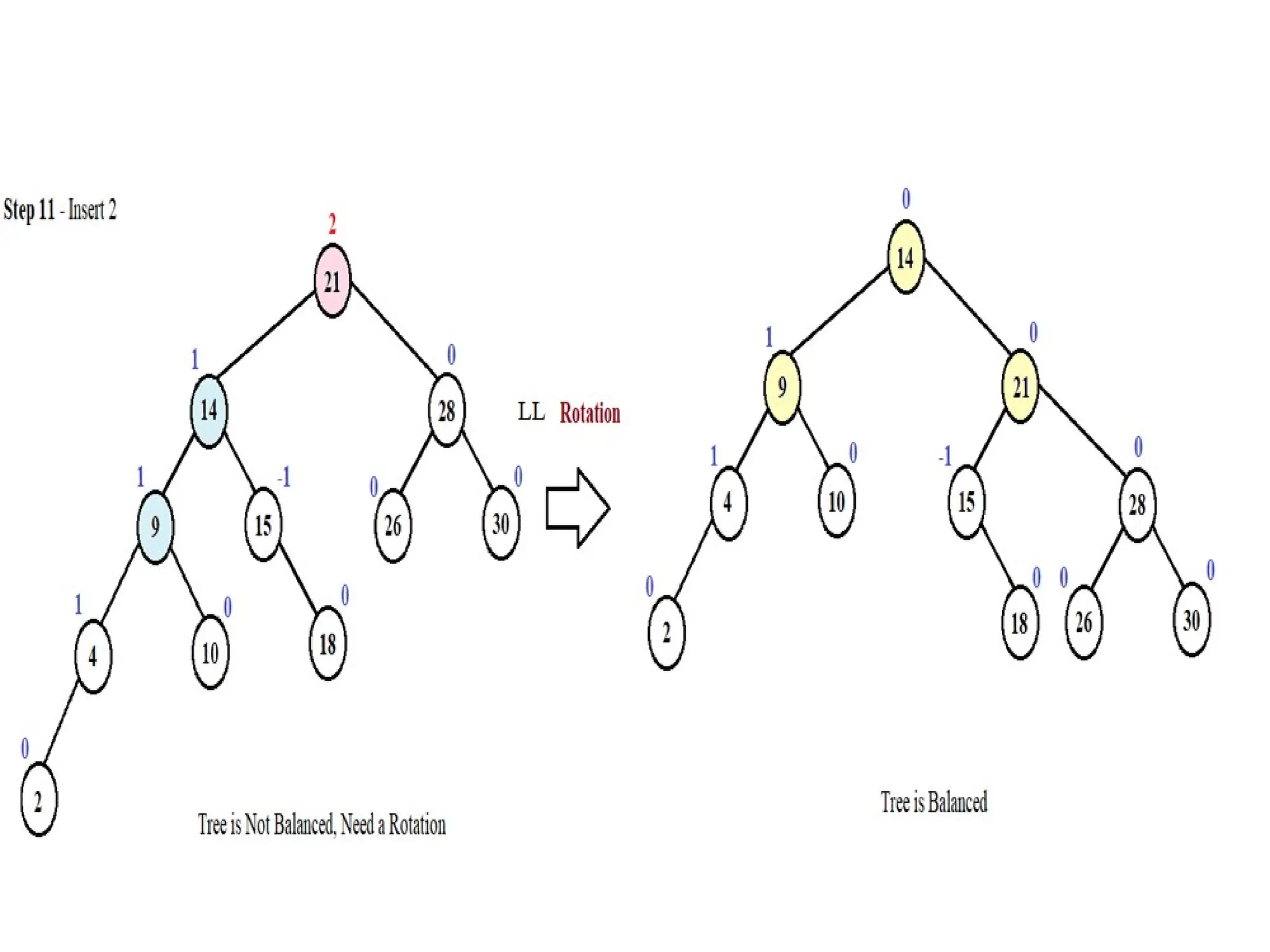
⚫Left-Left (LL) rotation
⚫Right-Right (RR) rotation
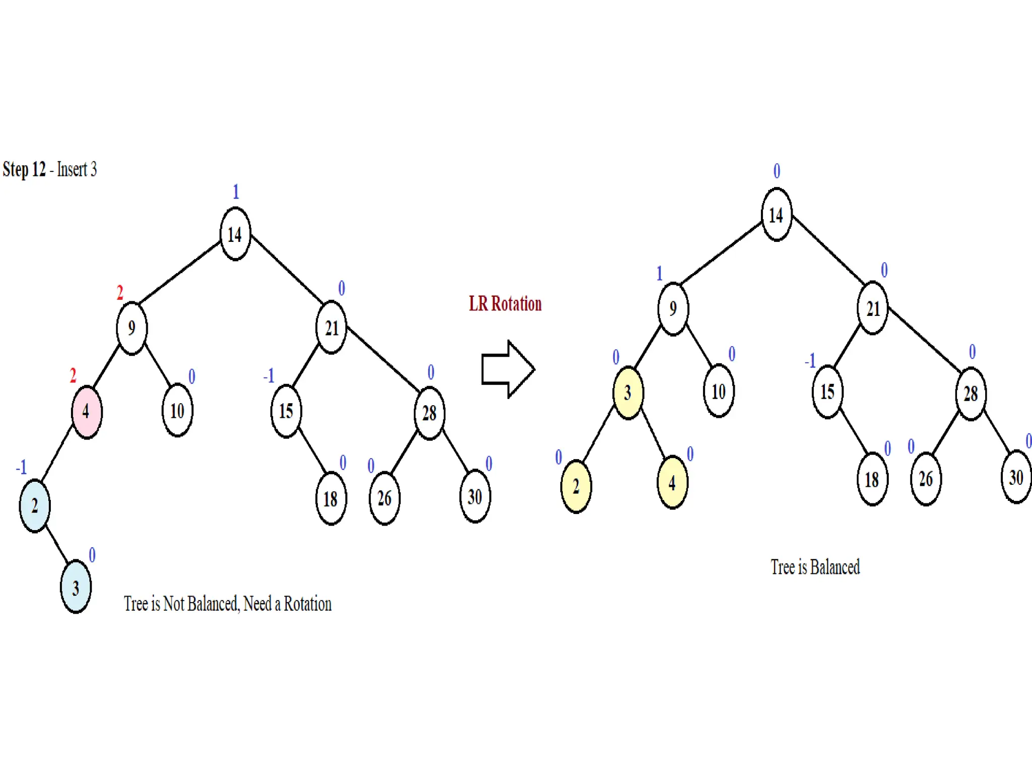
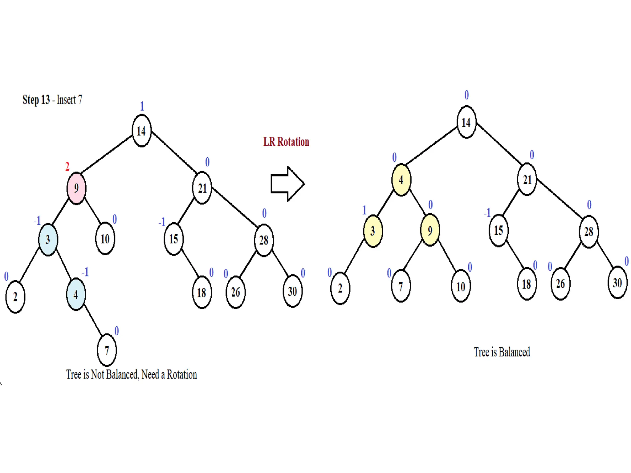
⚫Left-Right (LR) rotation
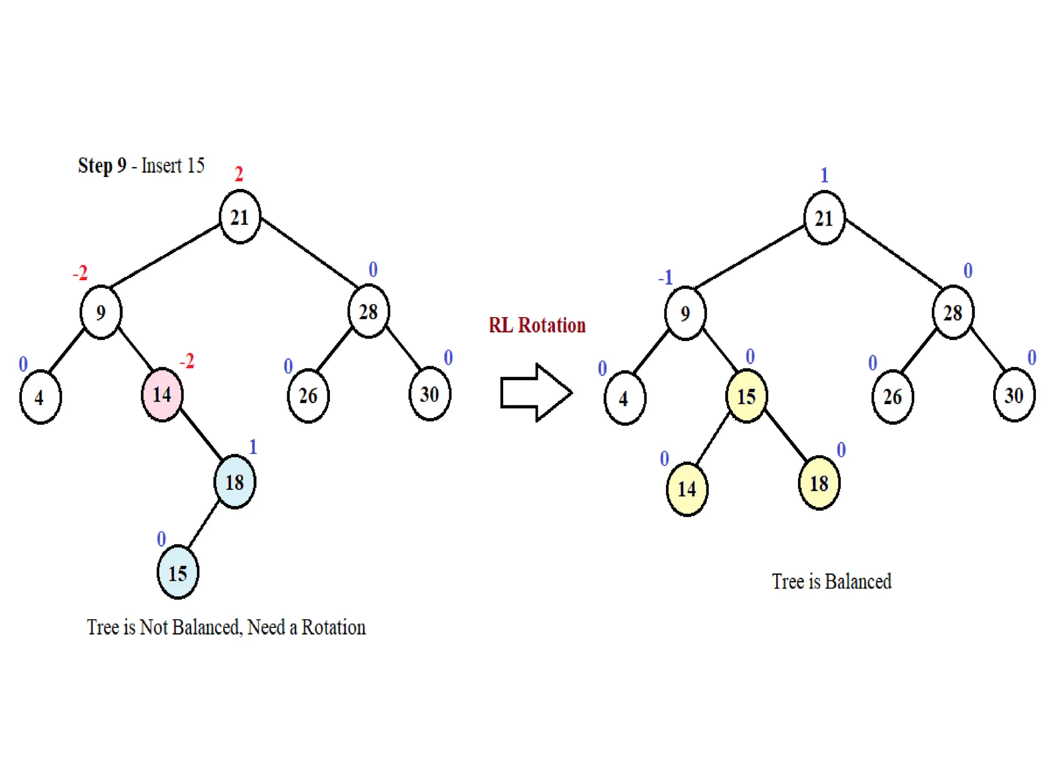
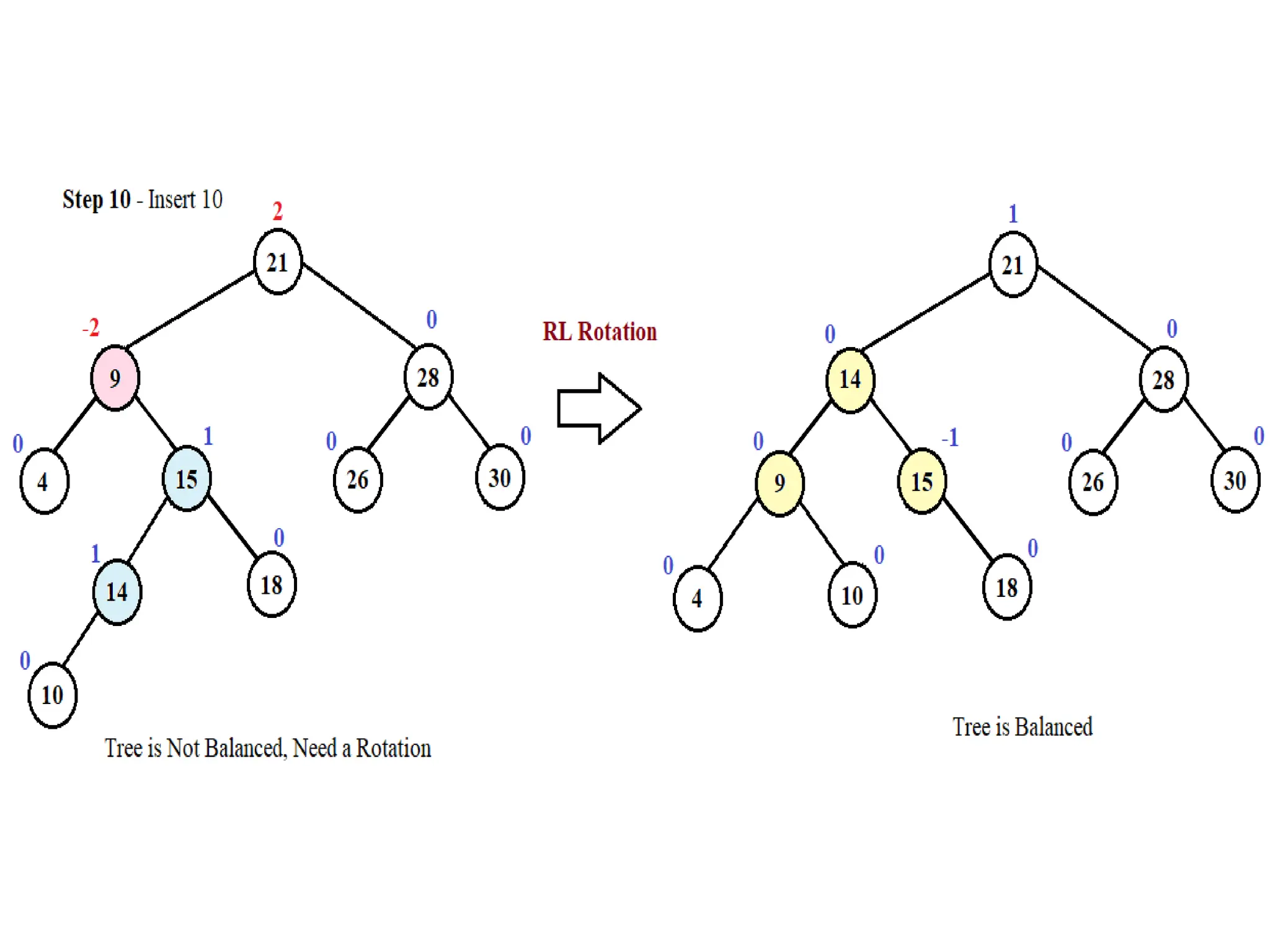
⚫Right-Left (RL) rotation
178.
⚫Assume that Ais the node which is unbalanced after
inserting a new node.
⚫LL Rotation: Inserted node is in the left subtree of
left subtree of node A.
⚫RR Rotation: Inserted node is in the right subtree of
right subtree of node A.
⚫LR Rotation: Inserted node is in the right subtree of
left subtree of node A.
⚫RL Rotation: Inserted node is in the left subtree of
right subtree of node A.
179.
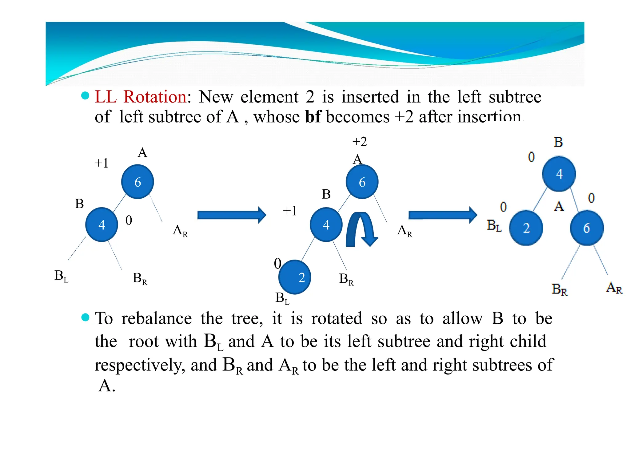
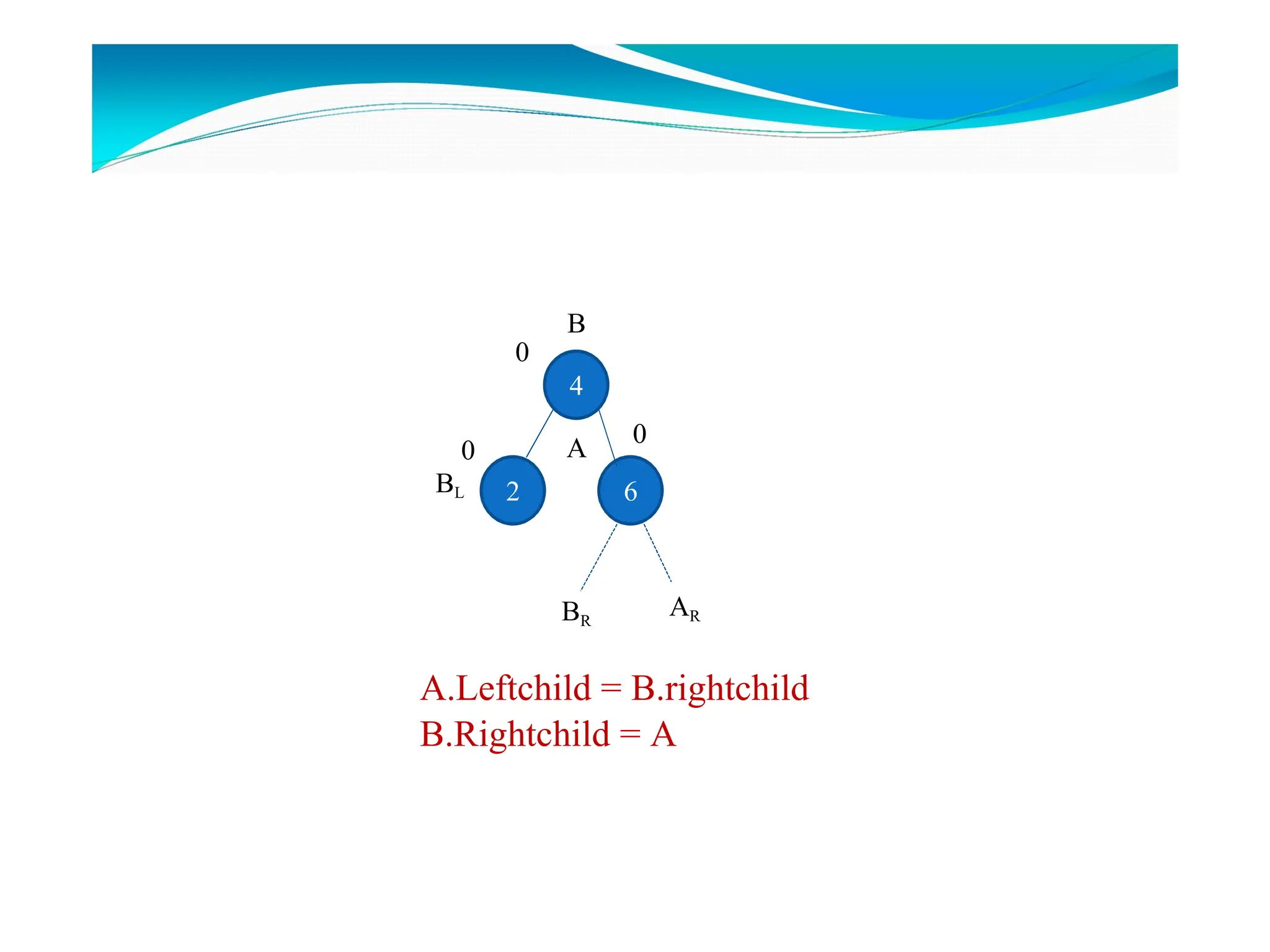
⚫LL Rotation: Newelement 2 is inserted in the left subtree
of left subtree of A , whose bf becomes +2 after insertion.
⚫To rebalance the tree, it is rotated so as to allow B to be
the root with BL and A to be its left subtree and right child
respectively, and BR and AR to be the left and right subtrees of
A.
6
4
A
B
0
+1
AR
BL
6
4
B
+2
A
AR
BR 2
+1
BL
BR
0
6
8
A
B
0
-1
AL
BR
BL
6
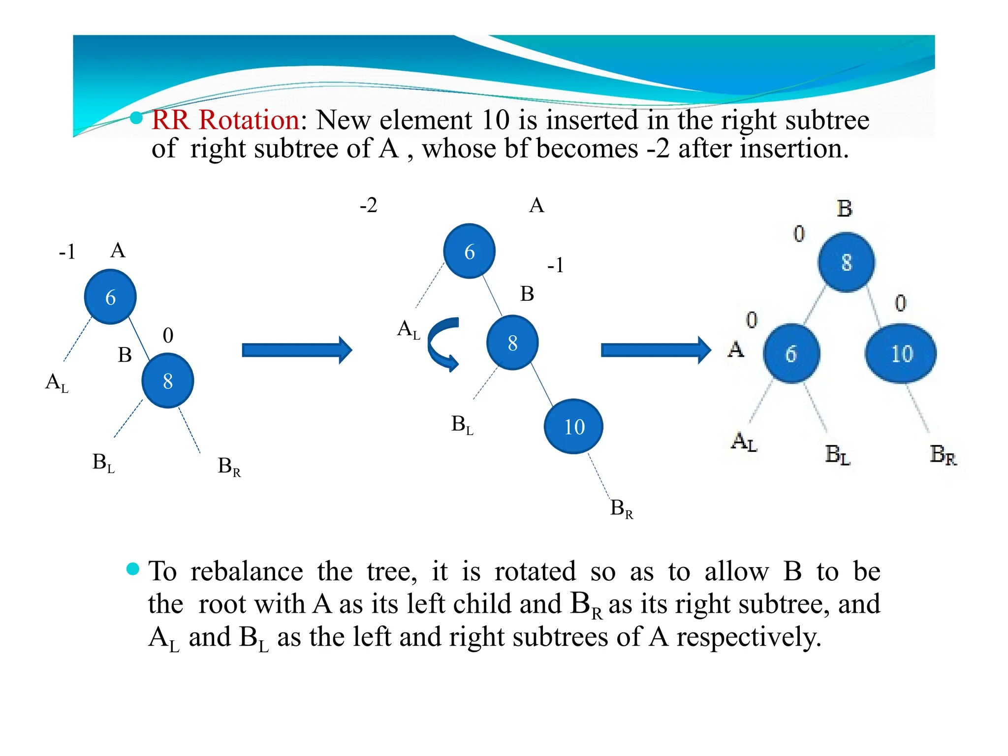
⚫RR Rotation: Newelement 10 is inserted in the right subtree
of right subtree of A , whose bf becomes -2 after insertion.
8
B
-1
AL
10
BL
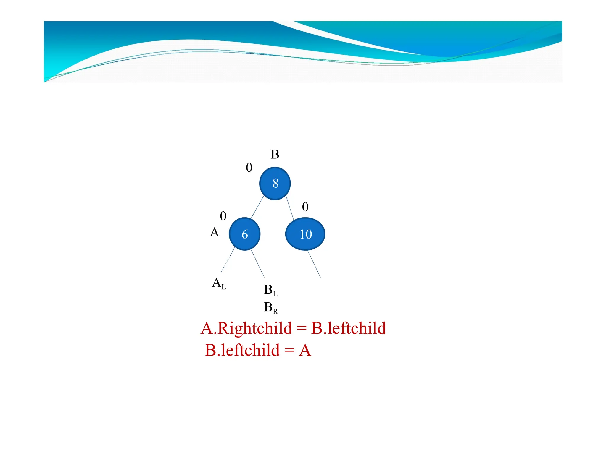
⚫To rebalance the tree, it is rotated so as to allow B to be
the root with A as its left child and BR as its right subtree, and
AL and BL as the left and right subtrees of A respectively.
BR
-2 A
• Create anAVL tree by inserting the elements
in the following order:
• 10,5,15,1,8,20,25,30,40,50
186.
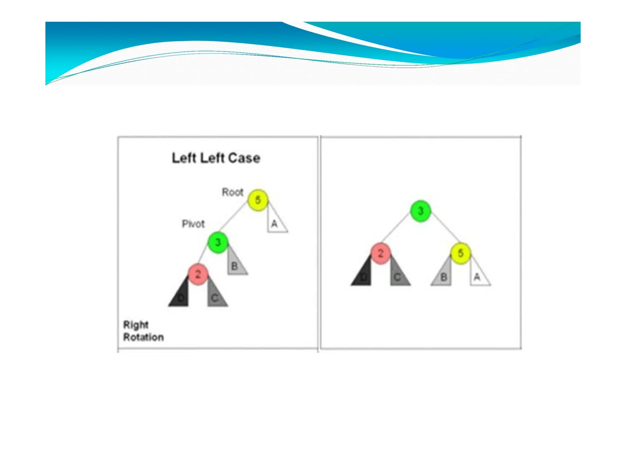
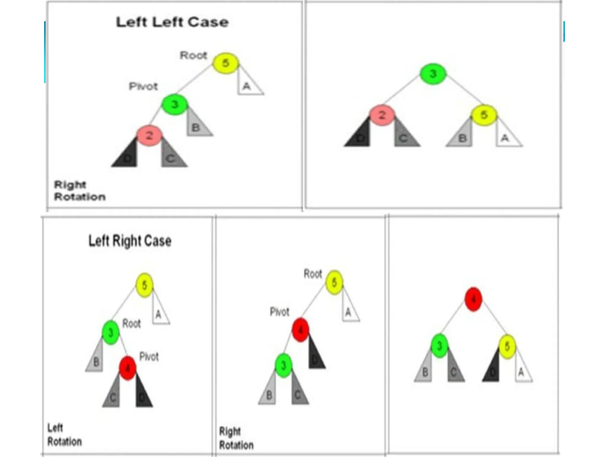
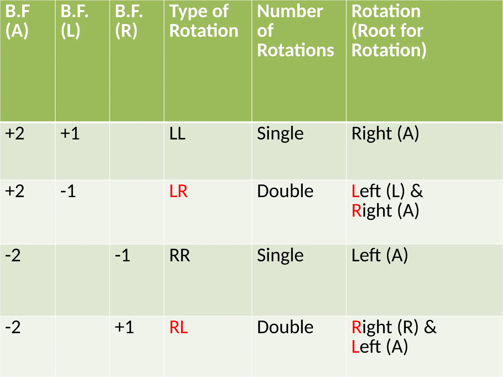
⚫Left-Left case andLeft-Right case:
⚫If the balance factor of A is 2, then the left subtree
outweighs the right subtree of the given node, and the
balance factor of the left child L must be checked. The right
rotation with A as the root is necessary.
⚫If the balance factor of L is +1, a single right rotation (with A
as the root) is needed (Left-Left case).
⚫If the balance factor of L is -1, two different rotations are
needed. The first rotation is a left rotation with L as the root.
The second is a right rotation with A as the root (Left-Right
case).
188.
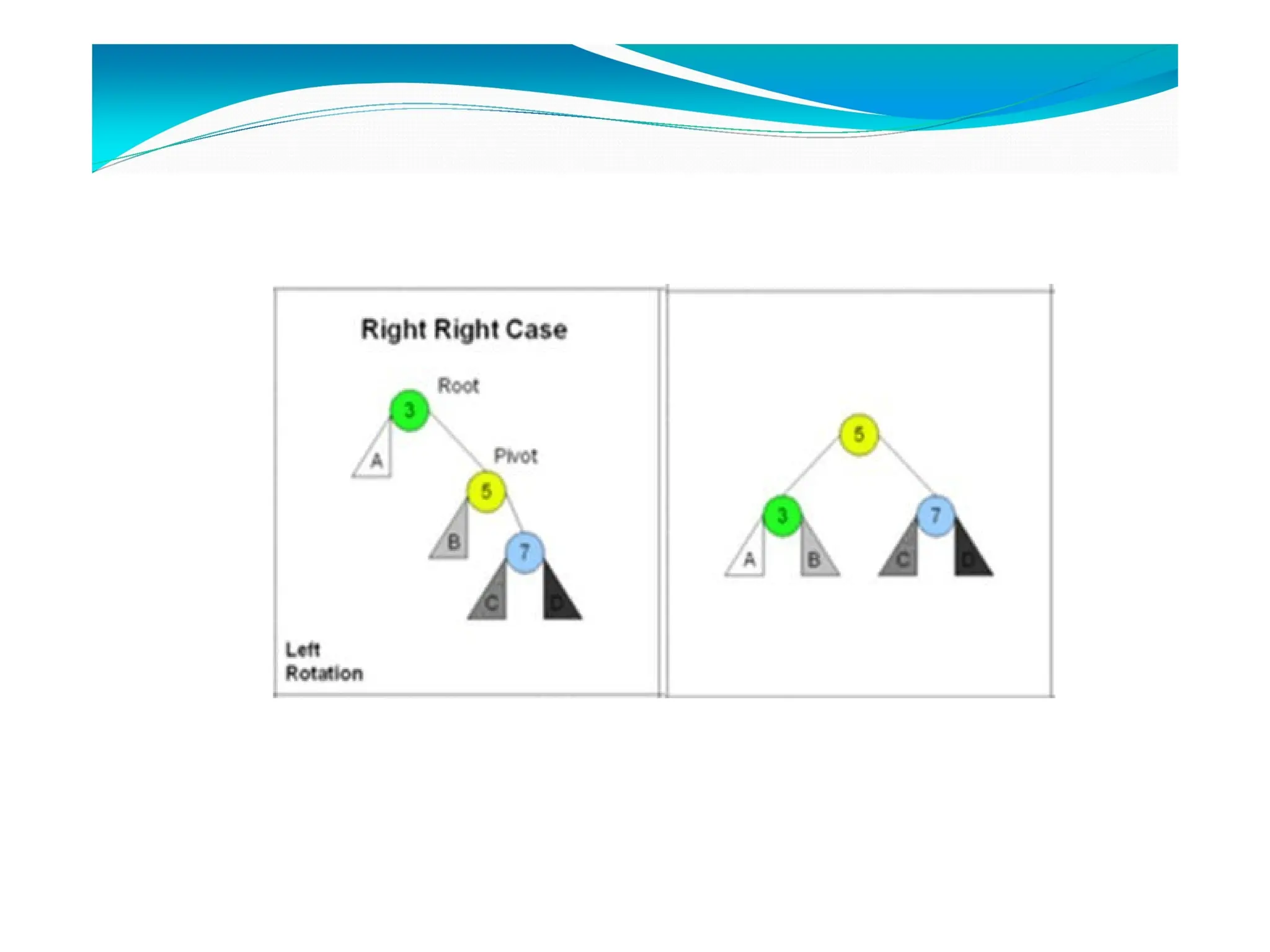
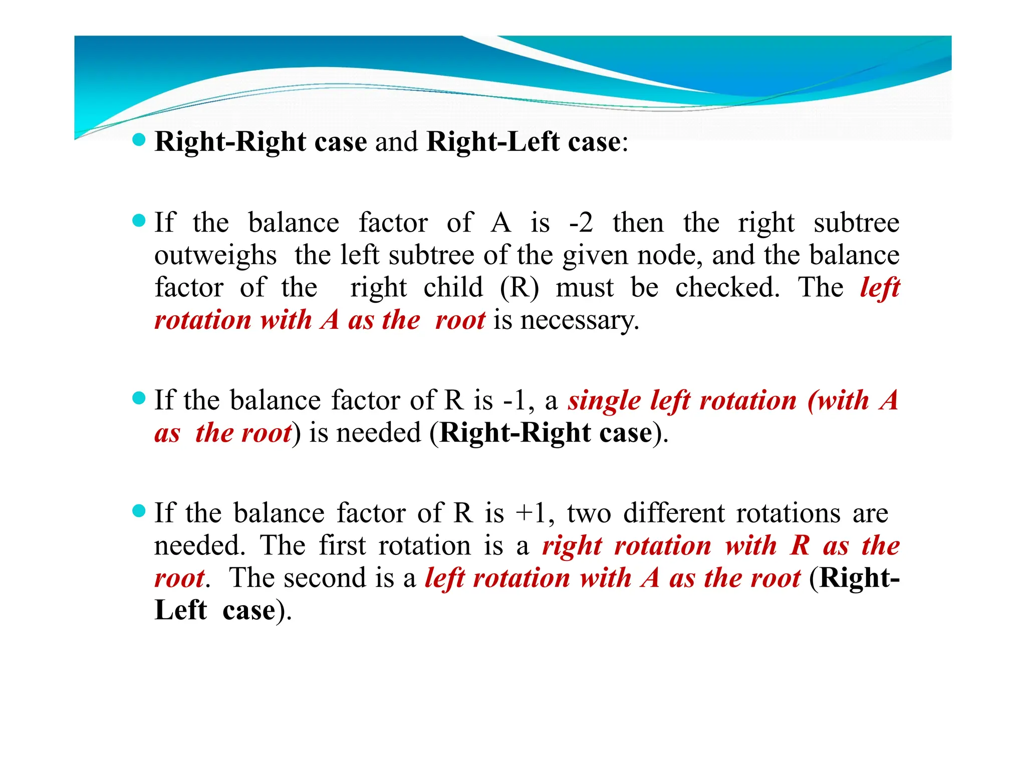
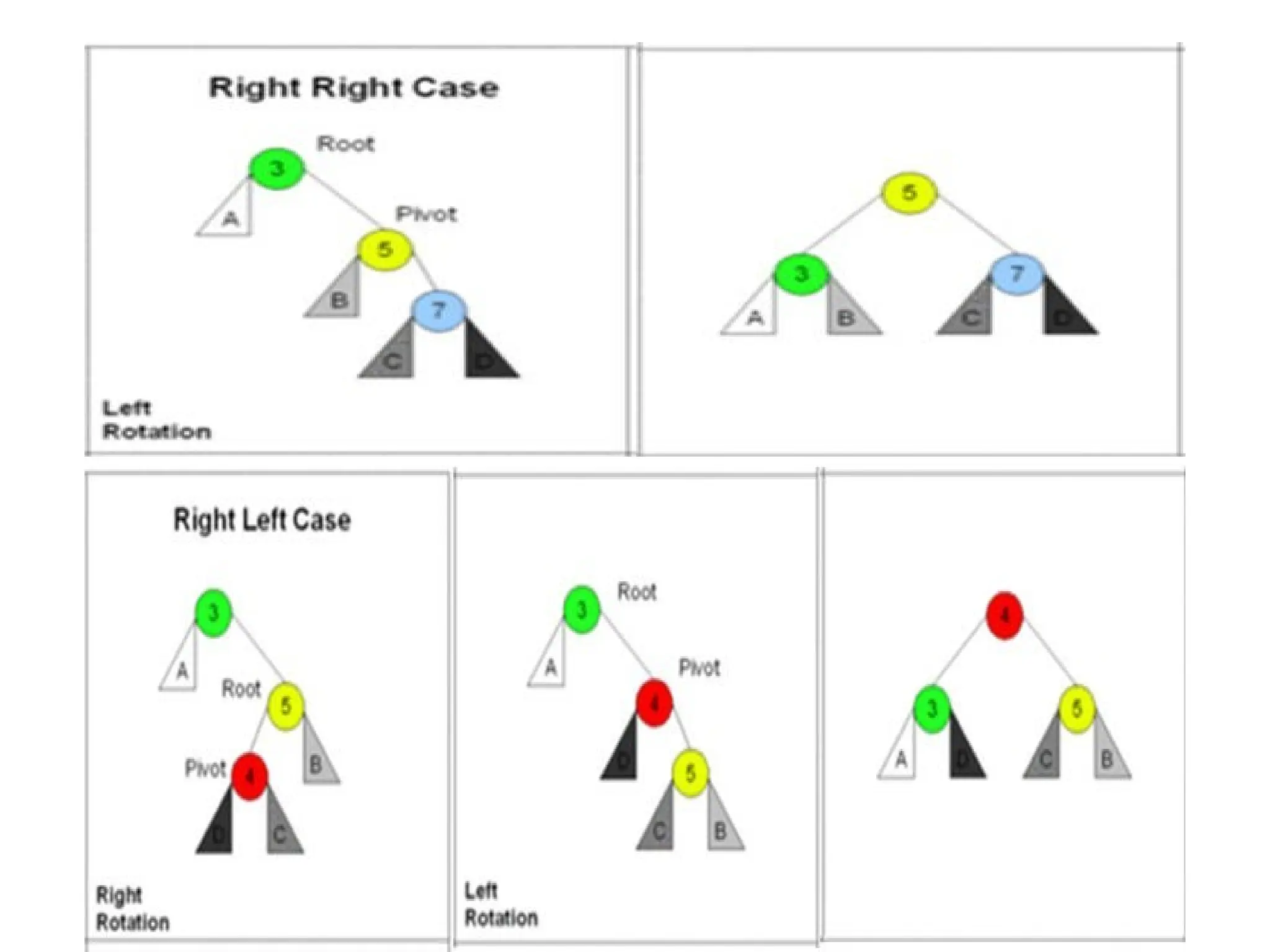
⚫Right-Right case andRight-Left case:
⚫If the balance factor of A is -2 then the right subtree
outweighs the left subtree of the given node, and the balance
factor of the right child (R) must be checked. The left
rotation with A as the root is necessary.
⚫If the balance factor of R is -1, a single left rotation (with A
as the root) is needed (Right-Right case).
⚫If the balance factor of R is +1, two different rotations are
needed. The first rotation is a right rotation with R as the
root. The second is a left rotation with A as the root (Right-
Left case).
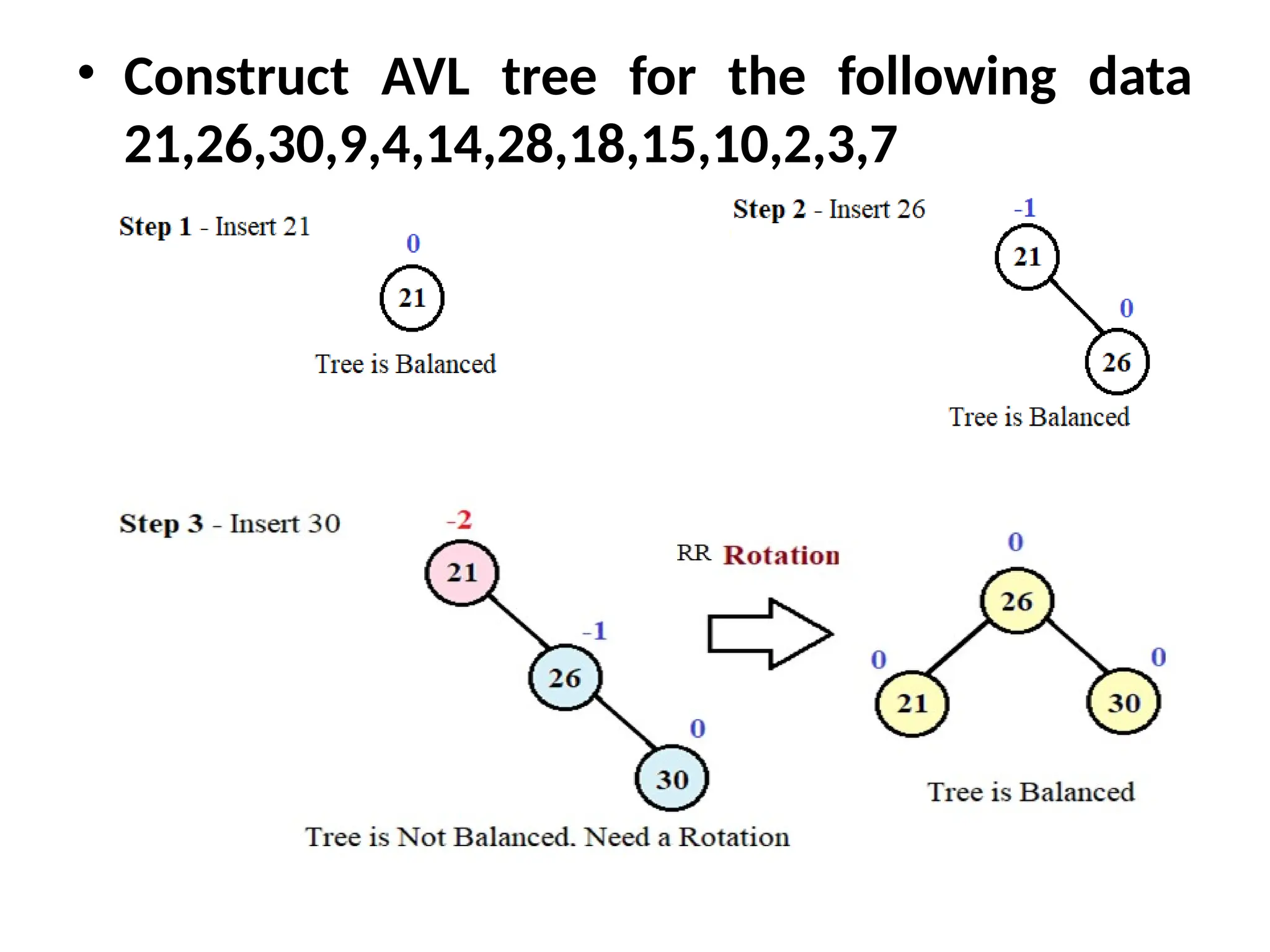
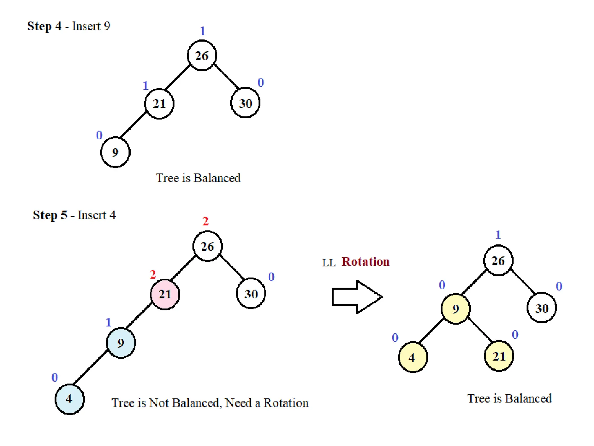
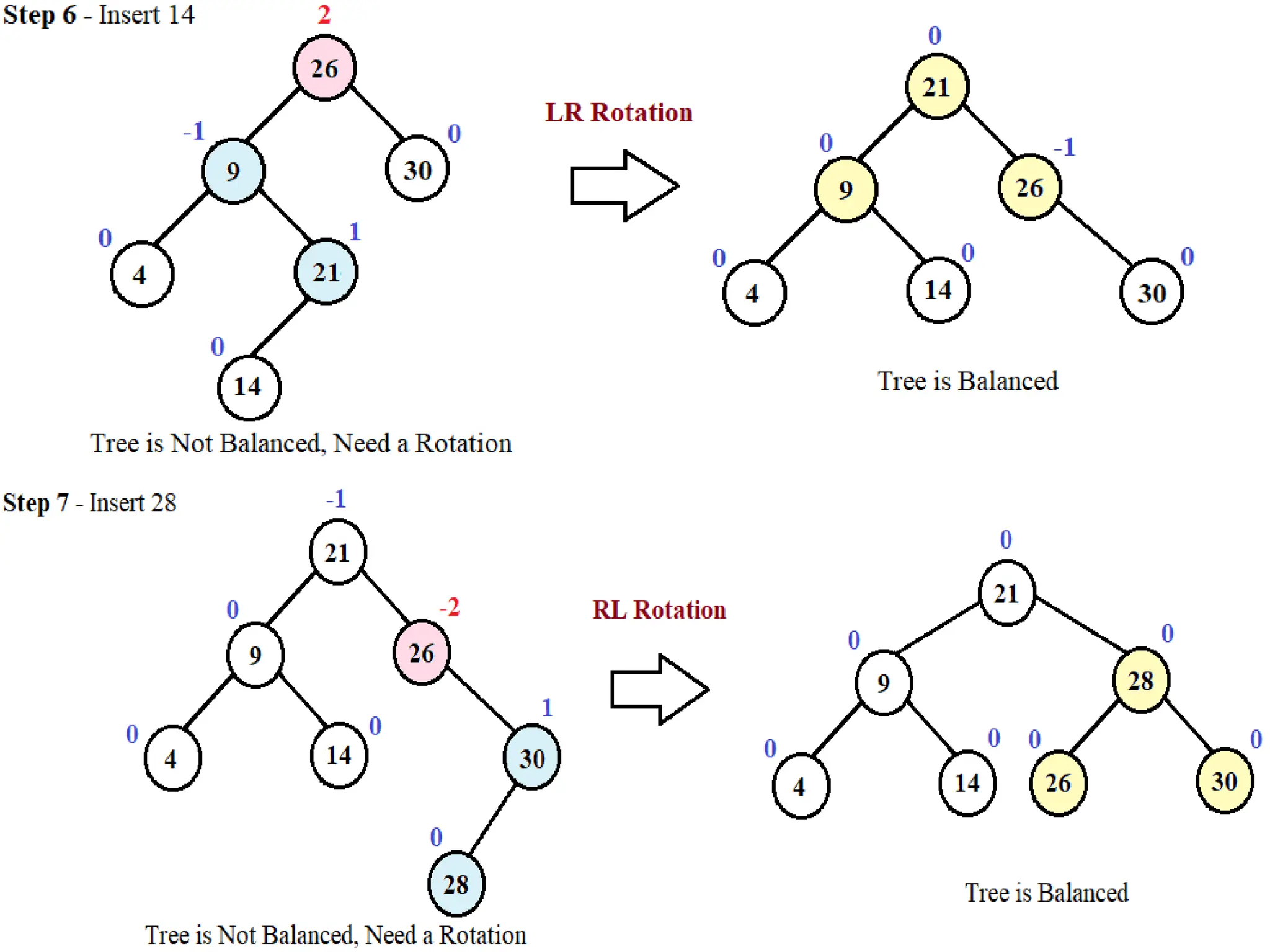
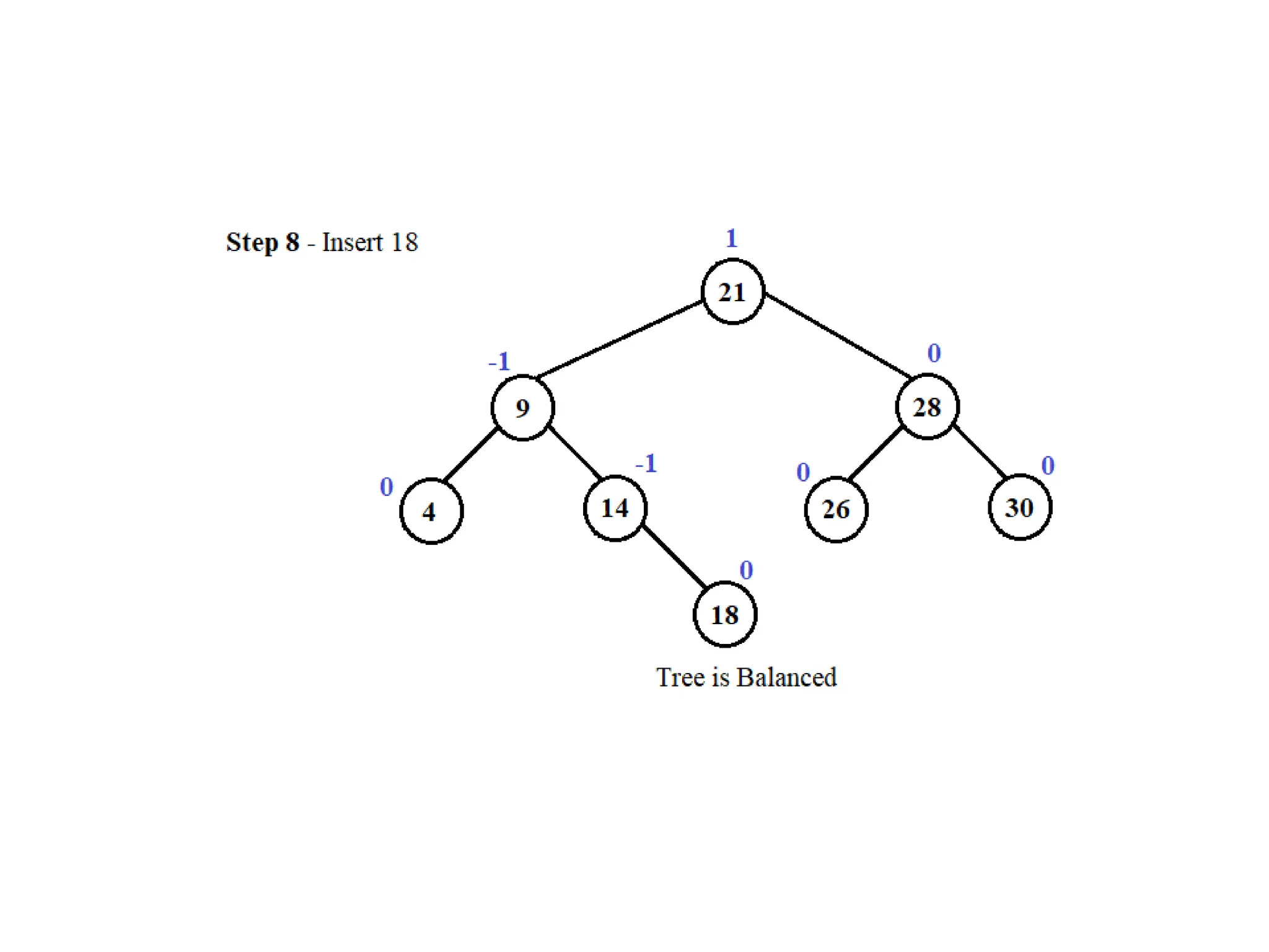
• Construct AVLtree for the following data
21,26,30,9,4,14,28,18,15,10,2,3,7
201.
AVL Tree
Deletion
⚫If thenode is a leaf or has only one child, remove it.
⚫Otherwise, replace it with either the largest in its left subtree
(inorder predecessor) or the smallest in its right subtree
(inorder successor), and remove that node.
⚫The node that was found as a replacement has at most one
subtree.
⚫After deletion, retrace the path back up the tree (parent of the
replacement) to the root, adjusting the balance factors as
needed.
202.
⚫The retracing canstop if the balance factor becomes −1
or
+1 indicating that the height of that subtree has
remained unchanged.
⚫If the balance factor becomes 0 then the height of the
subtree has decreased by one and the retracing needs to
continue.
⚫If the balance factor becomes −2 or +2 then the subtree
is unbalanced and needs to be rotated to fix it.
203.
Reference
⚫Sanjay Pahuja, ‘APractical Approach to Data
Structures and Algorithms’, First Ed. 2007.
⚫For Height Balanced Trees: AVL, B-Trees, refer:
⚫ Pg. 292 – 296, 301 – 315
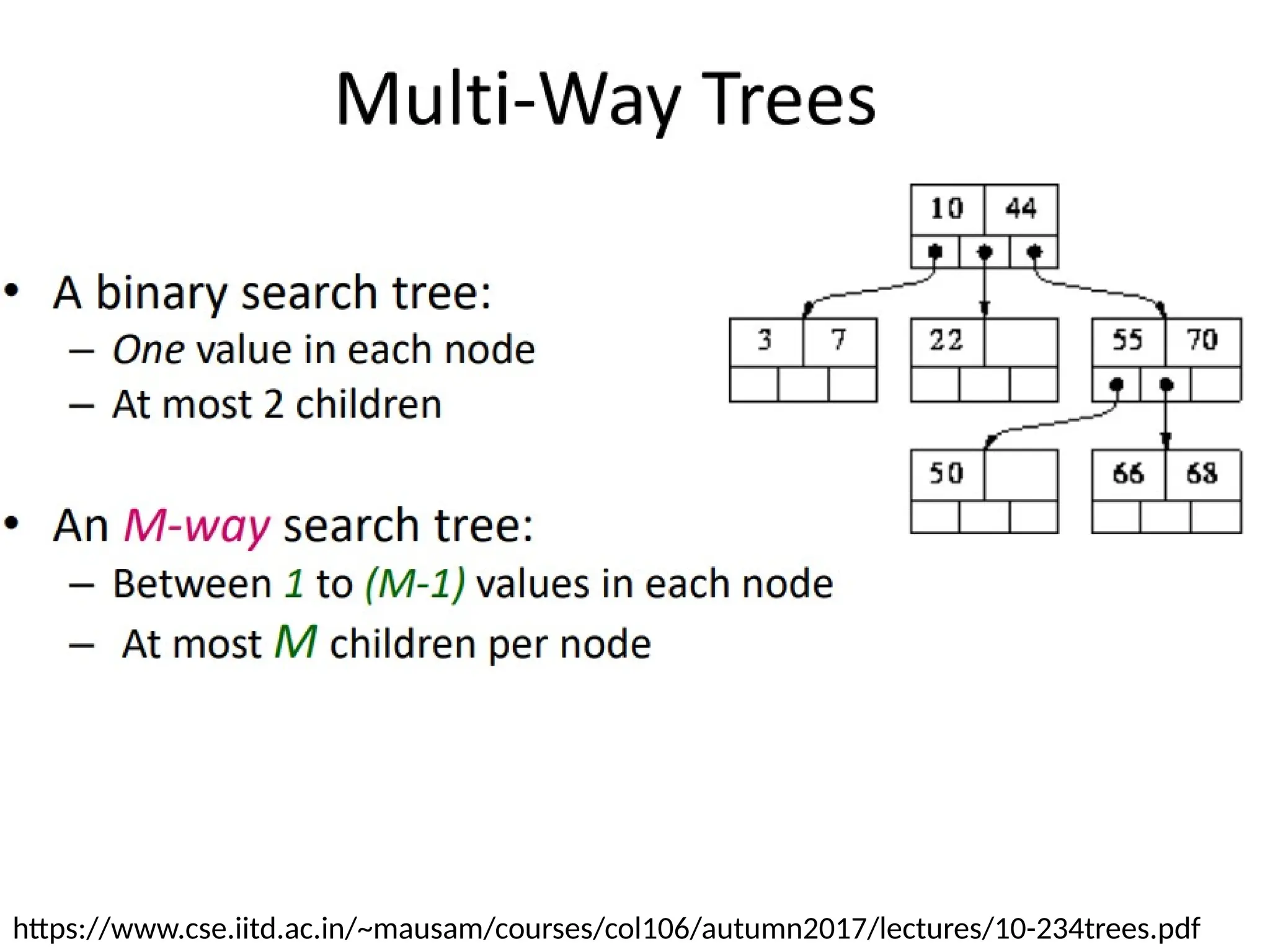
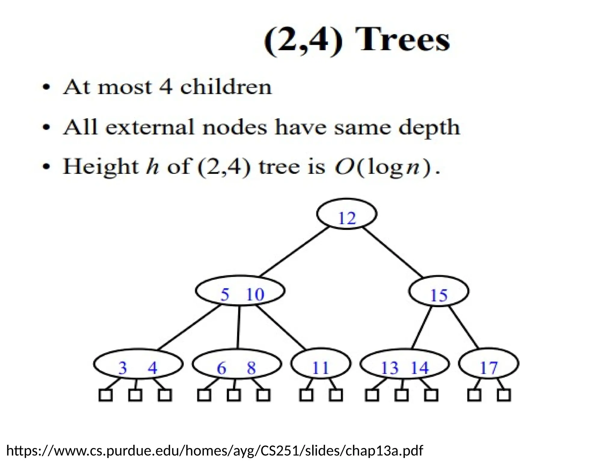
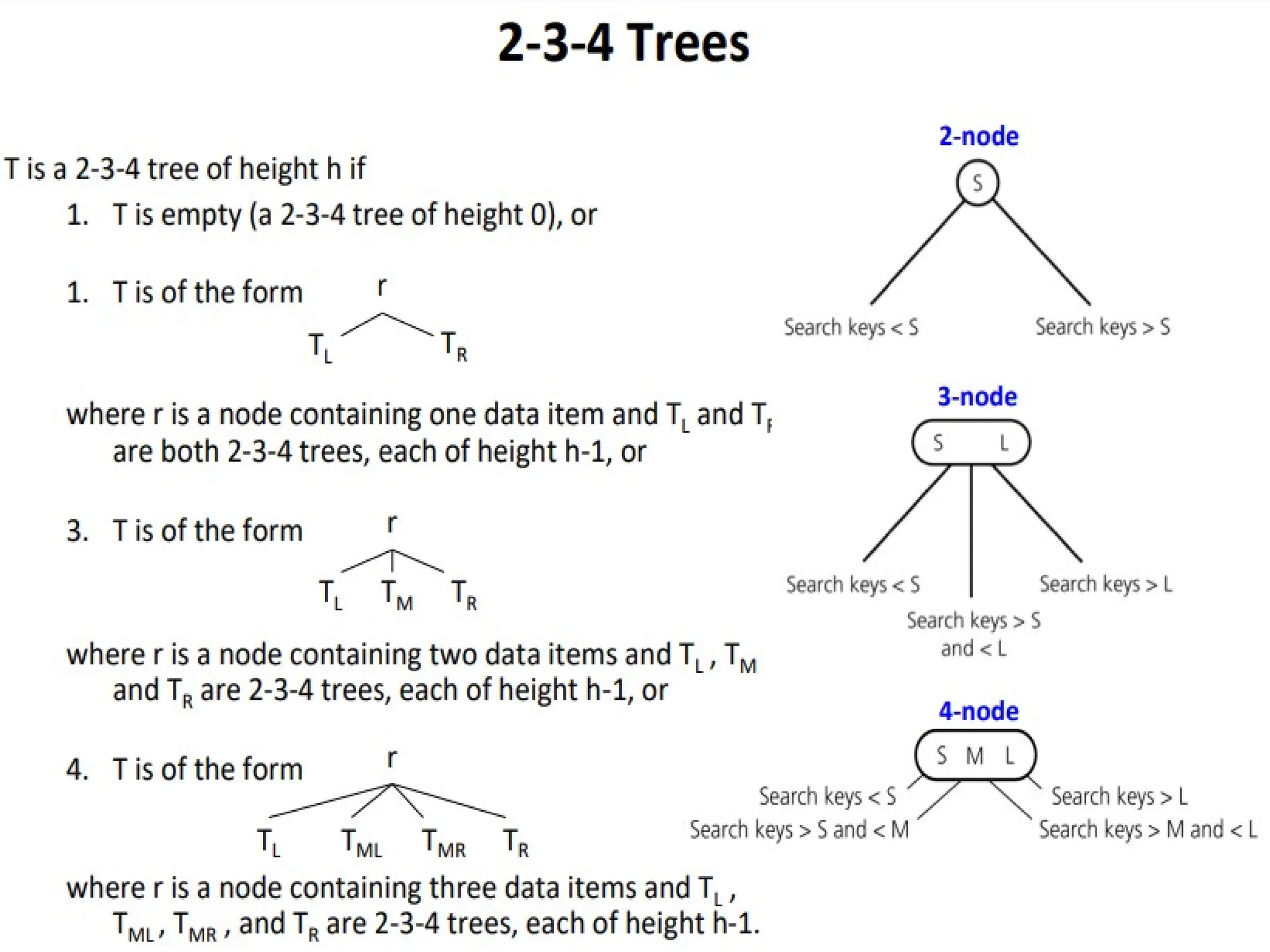
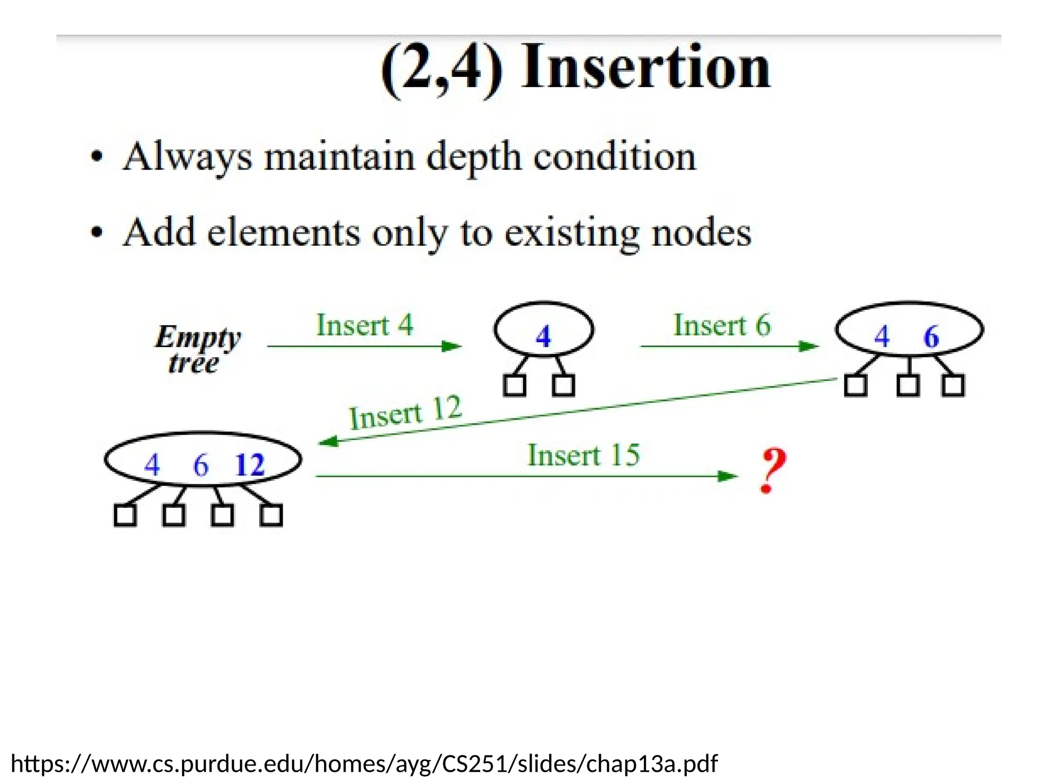
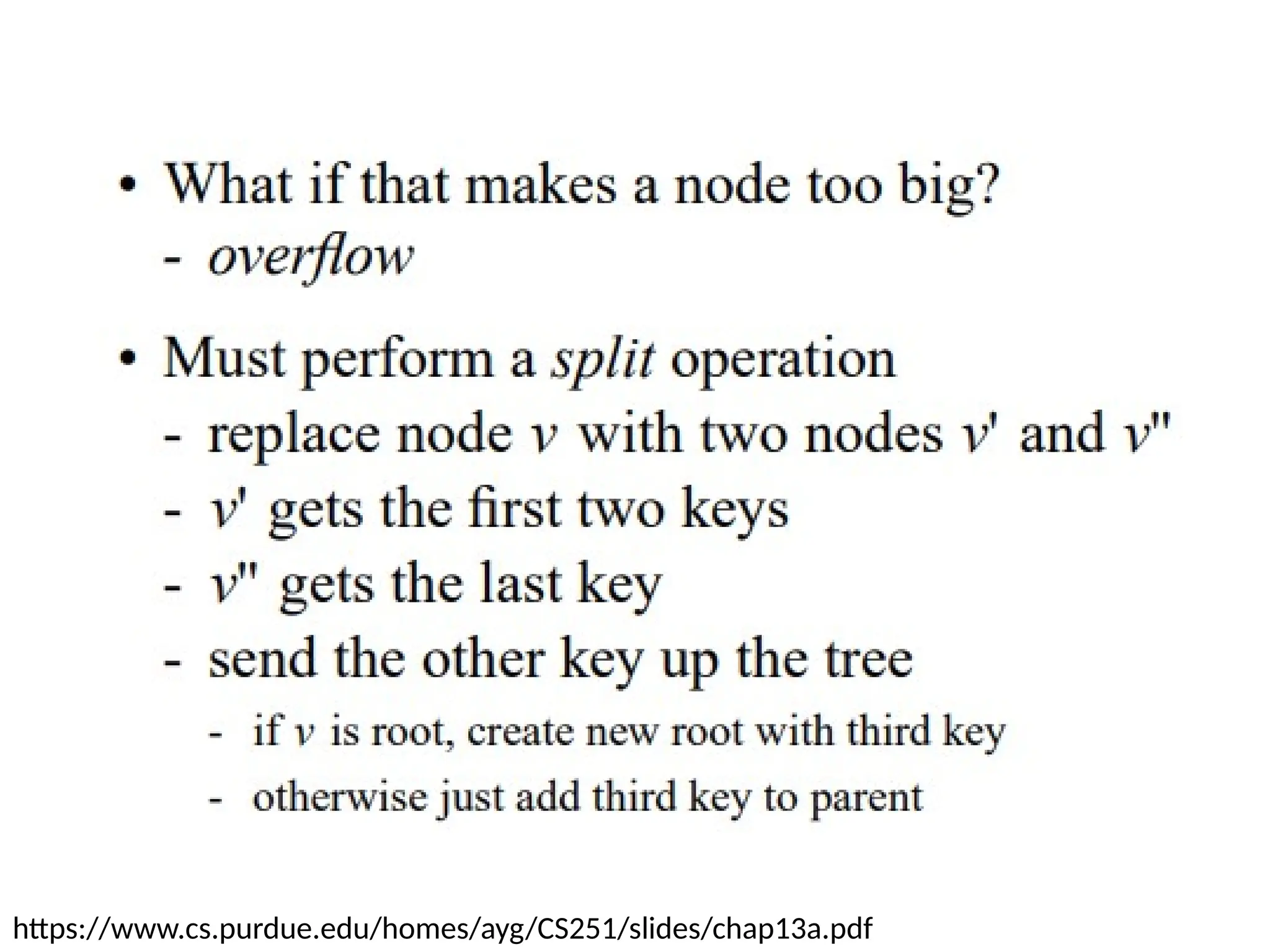
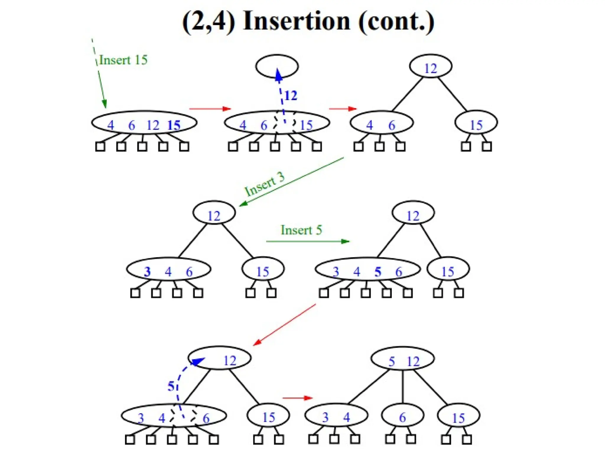
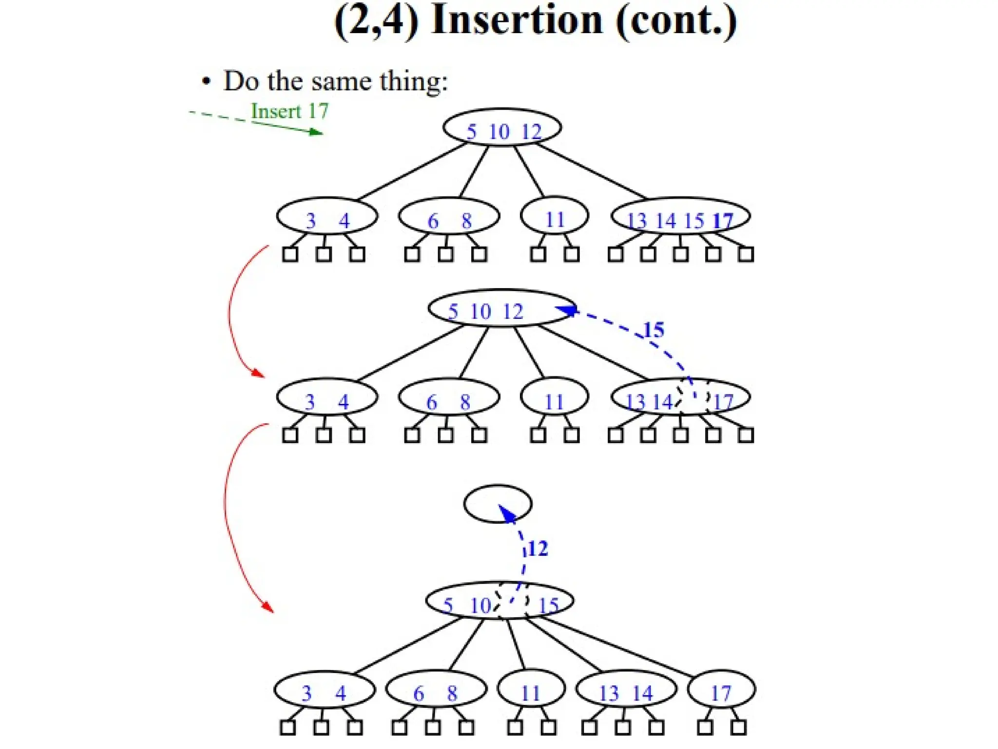
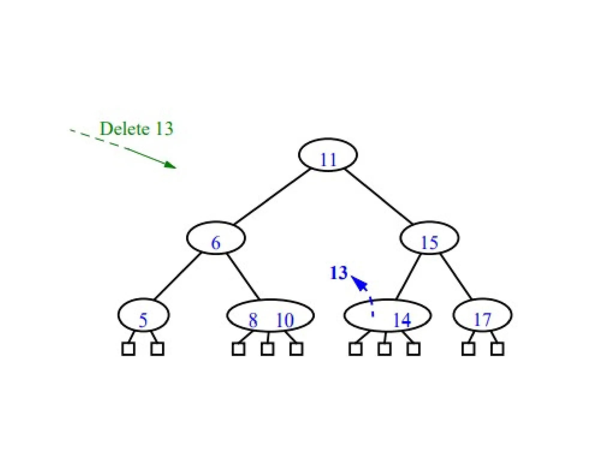
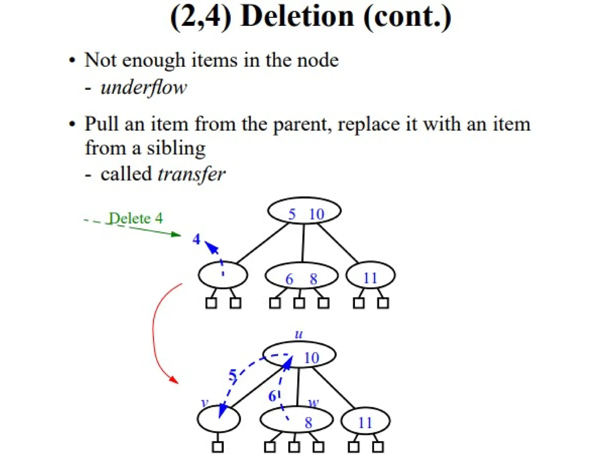
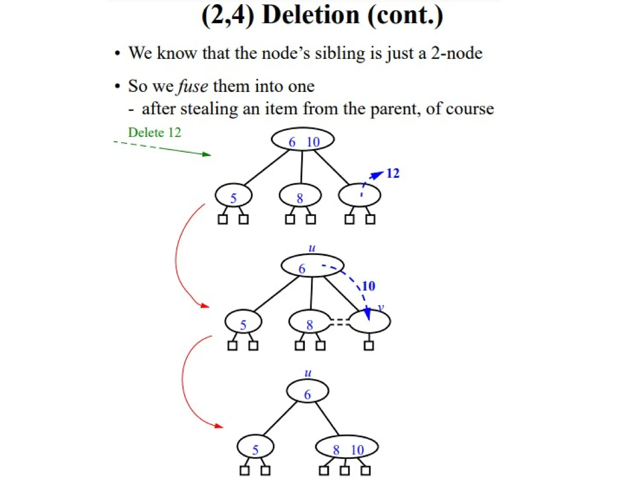
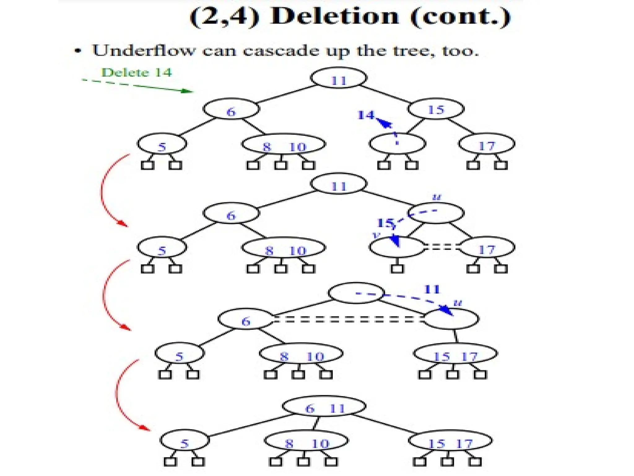
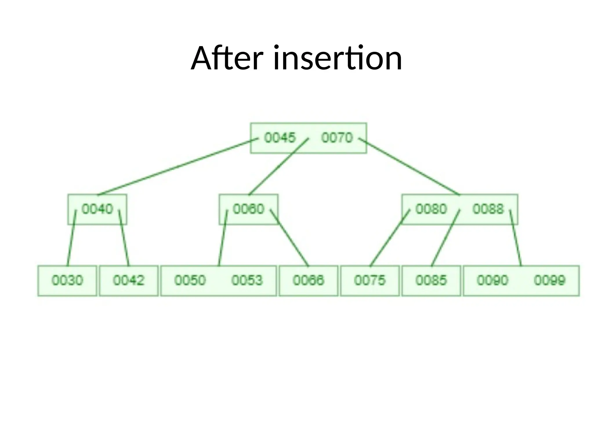
• Construct aB-Tree (2-4 tree) with the
following keys inserted in order.
• 30,99,70,60,40,66,50,53,45,42,88,75,80,85,90
• Assume that in case of a split 2nd
key is send to
parent, 1st
goes to left child, 3rd
, and 4th
keys go
to right child.
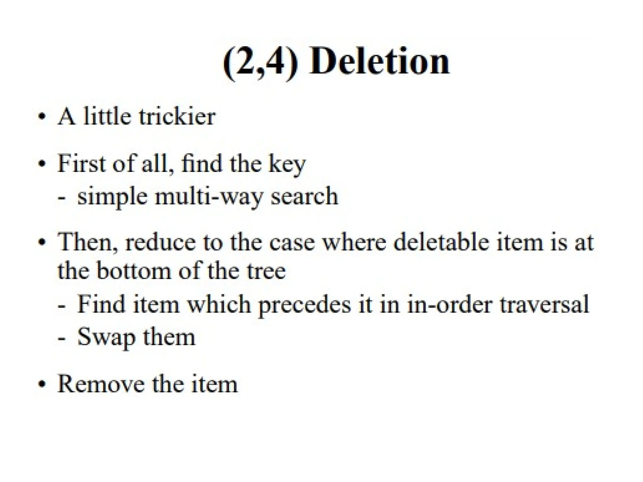
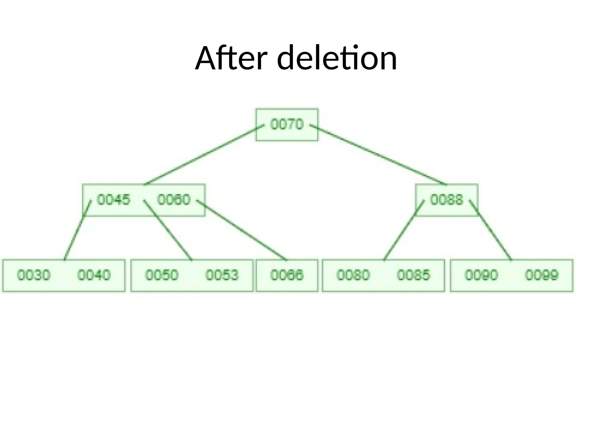
• Delete 42,75,80,45,90.
Hash Tables
• AHash table is defined as a data structure
used to insert, look up, and remove key-value
pairs quickly.
• It operates on the hashing, where each key is
translated by a hash function into a distinct
index in an array.
• The index functions as a storage location for
the matching value.
225.
• There aremajorly three components of hashing:
• Key: input to the hash function to determine an
index or location for storage of an item in a data
structure.
• Hash Function: function that maps the key to a
location in an array called a hash table. The index
is known as the hash index.
Most commonly used function:
hash (key) = (key%size)
• Hash Table: Hash table is a data structure that
maps keys to values using a special function called
a hash function. Hash stores the data in an
associative manner in an array where each data
value has its own unique index.
226.
Collision Resolution
• Collisionoccurs when two or more keys map to the
same hash value.
• There are mainly two methods to handle collision:
• Separate Chaining - Separate linked list for each key
• Open Addressing - All values are in hash table itself.
– Linear Probing
– Quadratic Probing
– Double Hashing