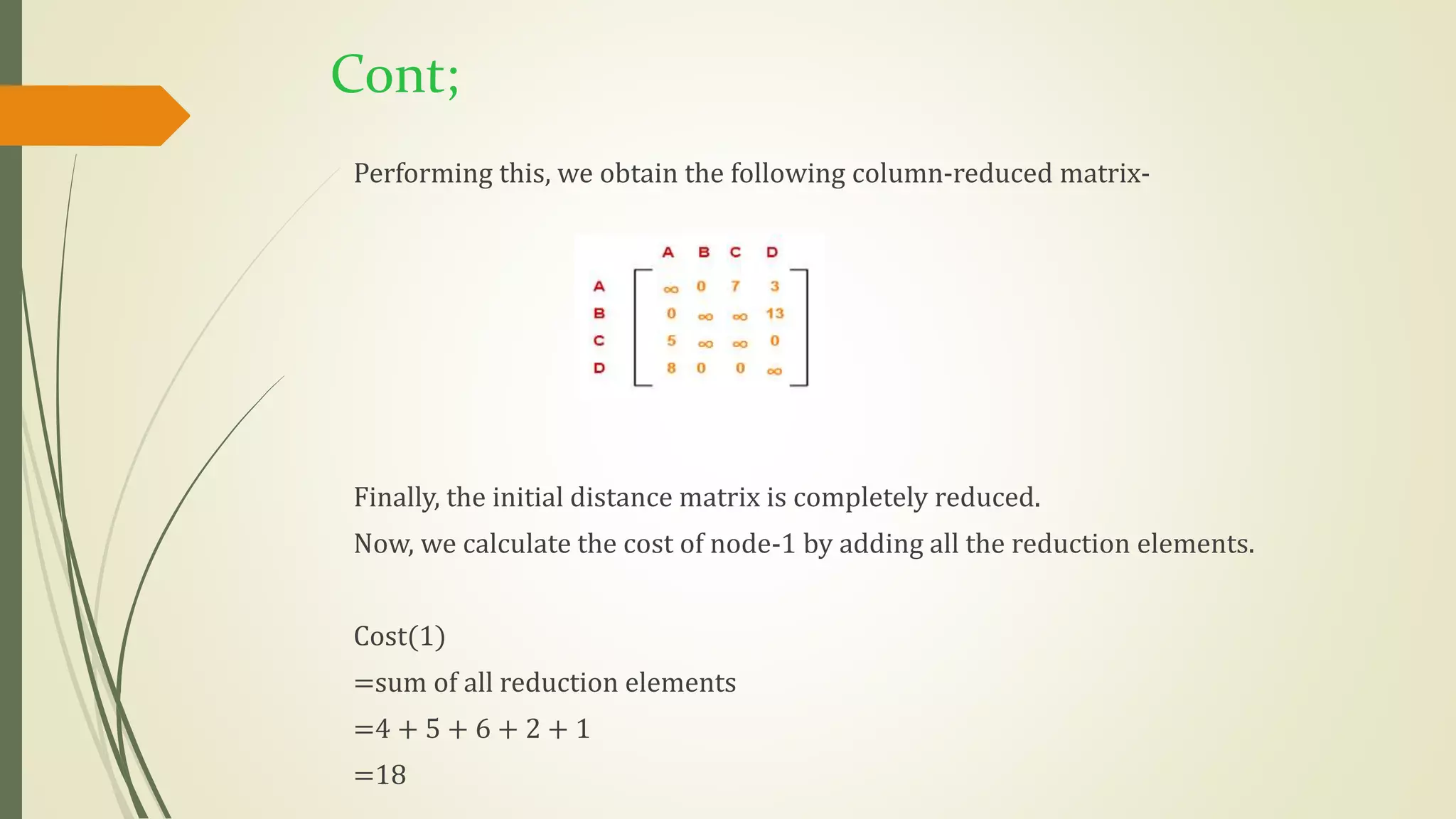
The document presents an overview of the Travelling Salesman Problem (TSP) and its solution using the Branch and Bound algorithm. It details the steps involved in determining the shortest route for a salesman visiting a set of cities and returning to the starting point, including cost calculations and matrix reductions. The final optimal path and its cost are identified, along with efficiency considerations for implementing Branch and Bound methods.


![Cont;
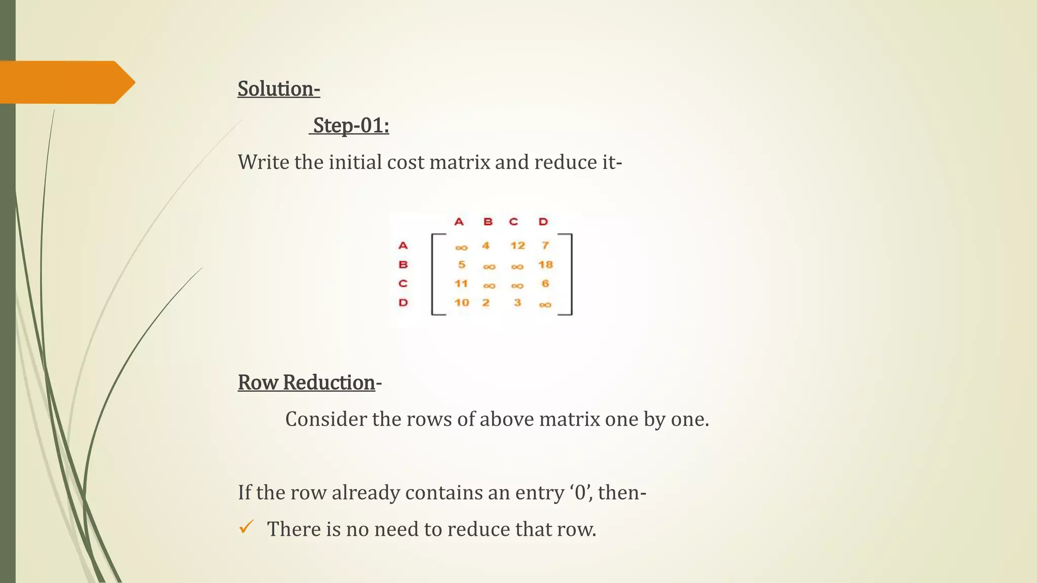
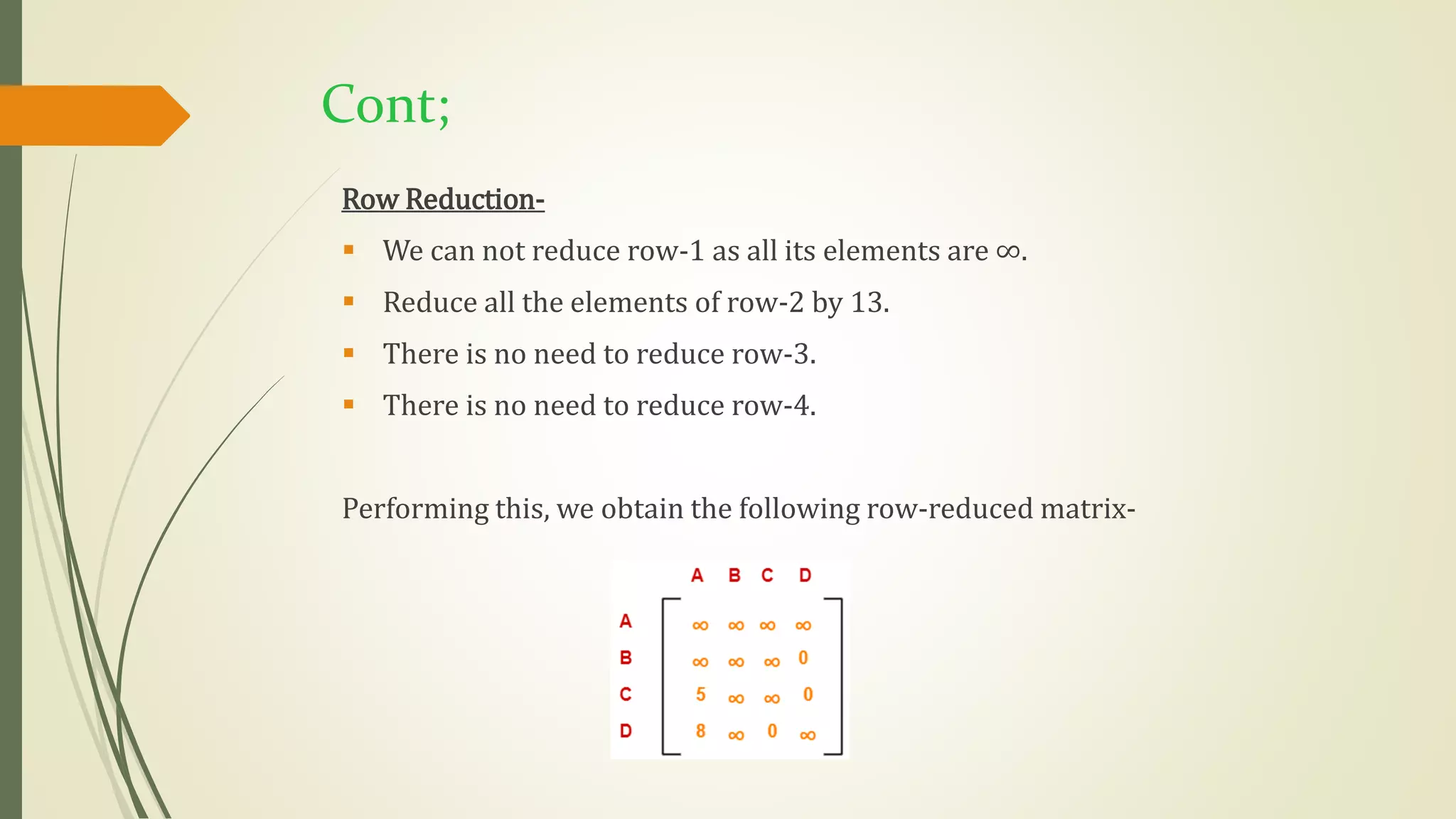
Step-02:
o We consider all other vertices one by one.
o We select the best vertex where we can land upon to minimize the tour cost.
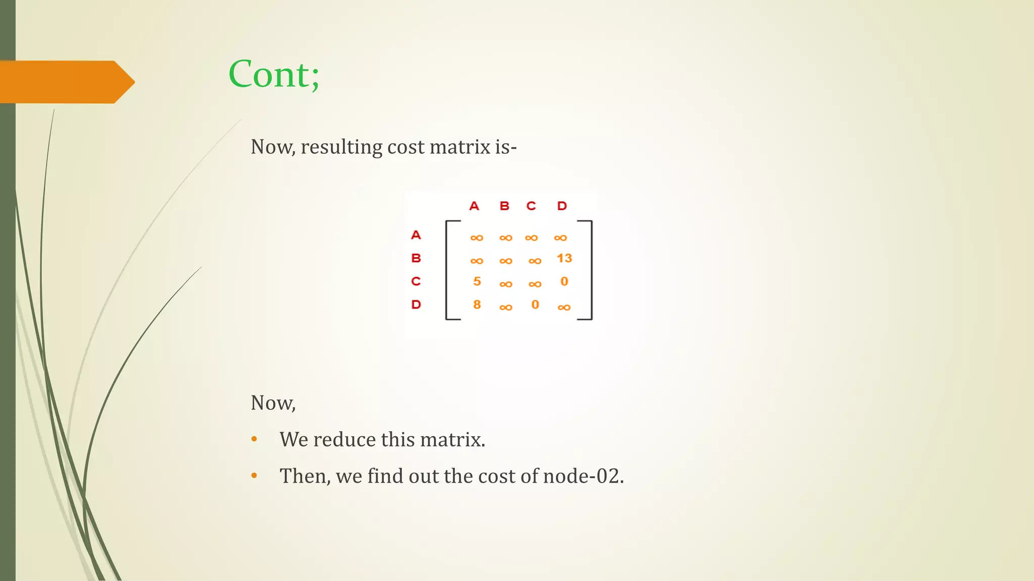
Choosing To Go To Vertex-B: Node-2(Path A B)
• From the reduced matrix of step-1, M[A,B] = 0
• Set row-A and column-B to ∞
• Set M[B,A] = ∞](https://image.slidesharecdn.com/datastructuresandalgorithms-220121073713/75/Data-structures-and-algorithms-11-2048.jpg)
![Cont;
Finally, the matrix is completely reduced.
Now, we calculate the cost of node-2.
Cost(2)
=Cost(1) + Sum of reduction elements + M[A,B]
=18 + (13 + 5) +0
=36
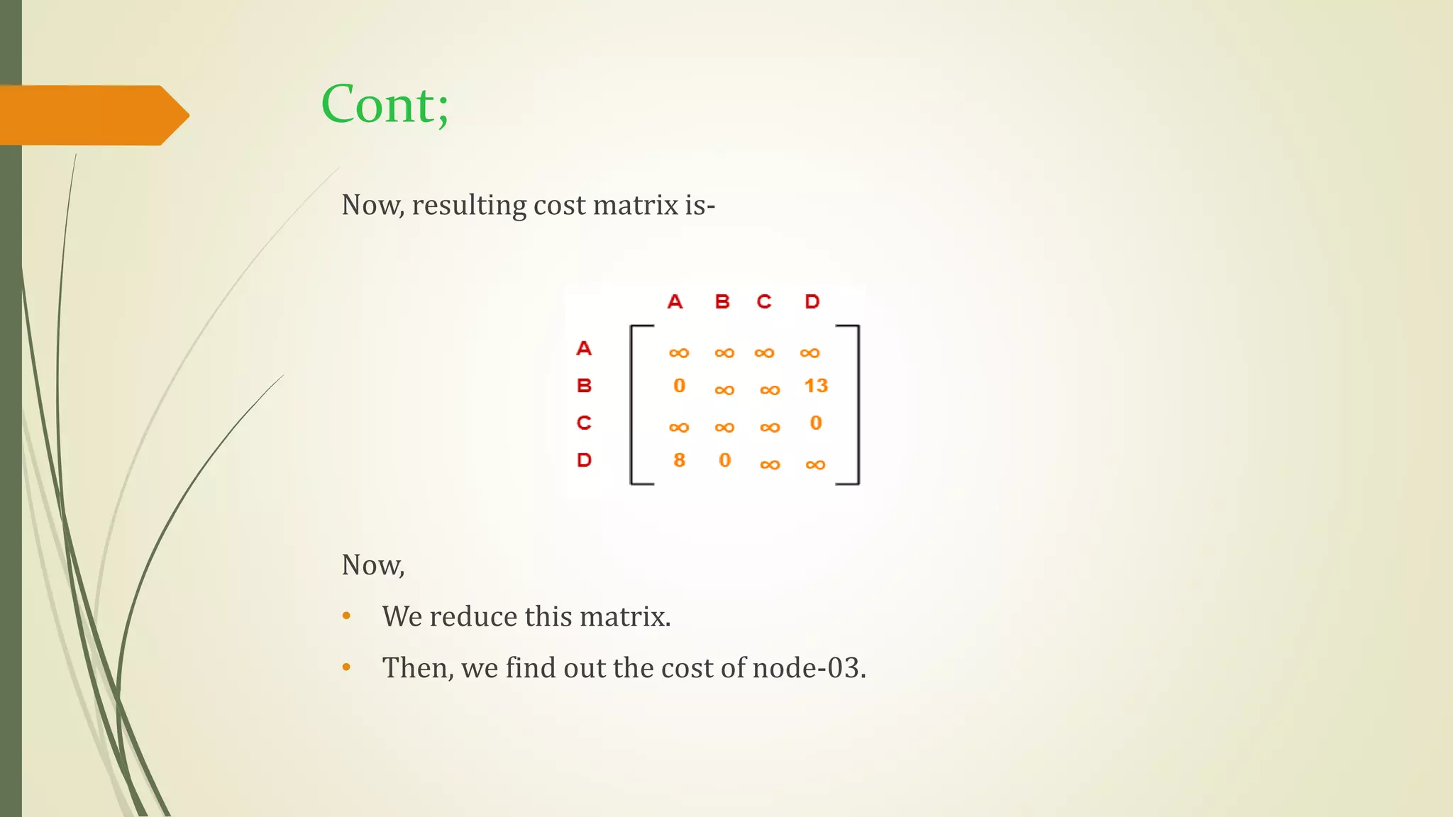
Choosing To Go To Vertex-C: Node-3 (Path A C)
From the reduced matrix of step-01,M[A,C]=7
Set row-A and column-C to ∞.
Set M[C,A] = ∞.](https://image.slidesharecdn.com/datastructuresandalgorithms-220121073713/75/Data-structures-and-algorithms-15-2048.jpg)
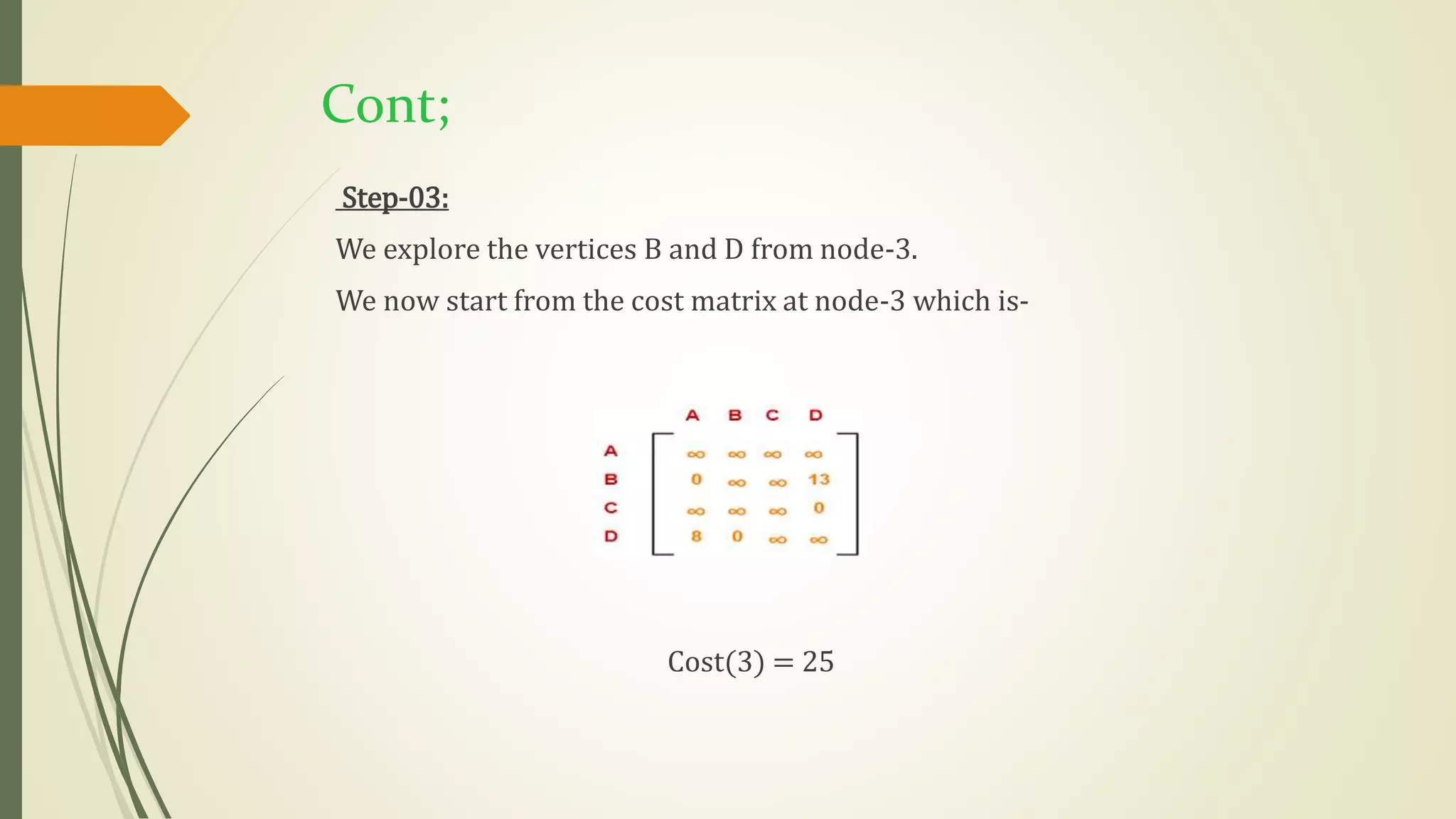
![Cont;
Finally, the matrix is completely reduced.
Now, we calculate the cost of node-3.
Cost(3)
=Cost(1) + Sum of reduction elements + M[A,C]
=18 + 0 + 7
=25
Choosing To Go To Vertex-D: Node-4 (Path A D)
• From the reduced matrix of step-01,M[A,D] = 3
• Set row-A and column-D to ∞.
• Set M[D,A] = ∞.](https://image.slidesharecdn.com/datastructuresandalgorithms-220121073713/75/Data-structures-and-algorithms-18-2048.jpg)
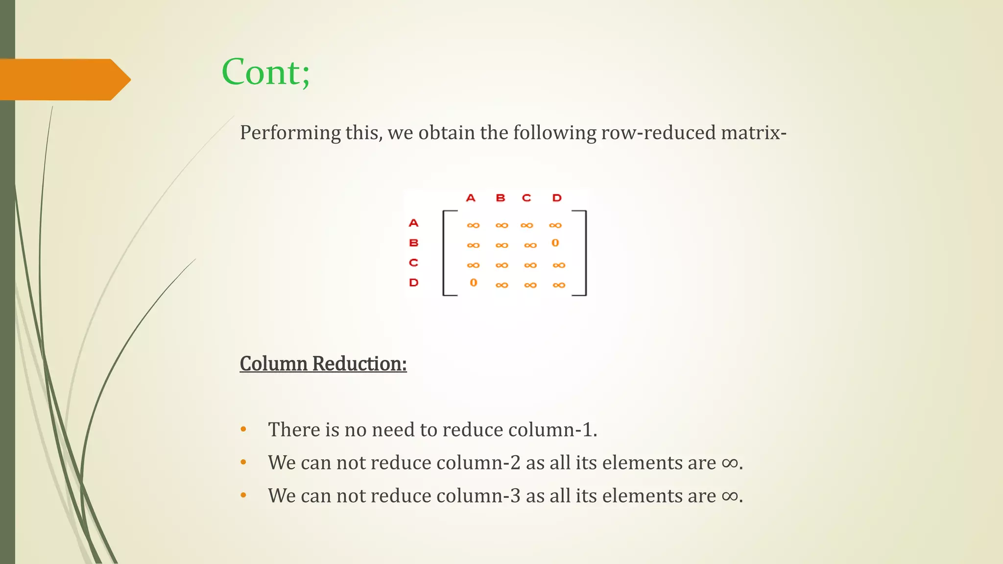
![Cont;
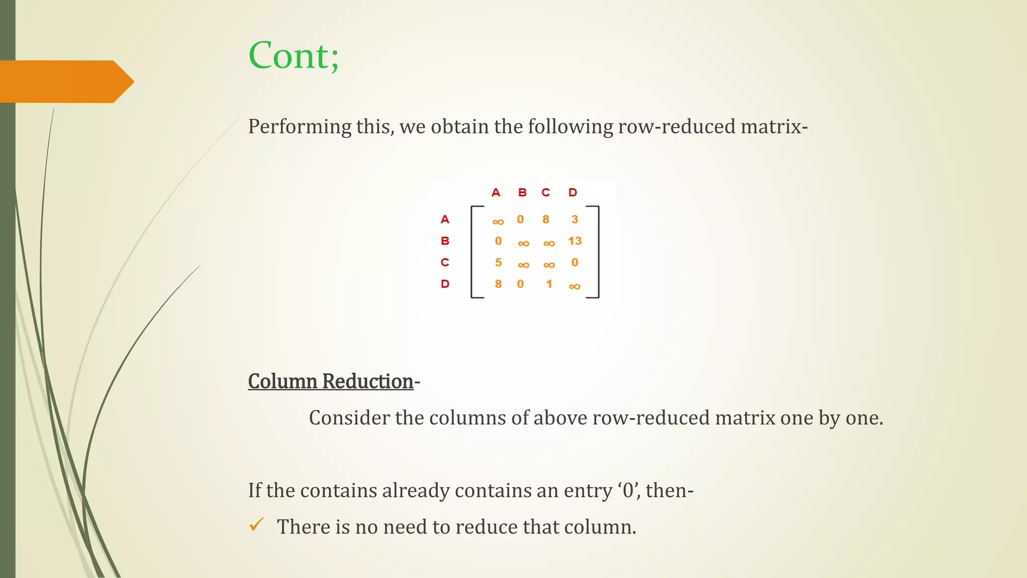
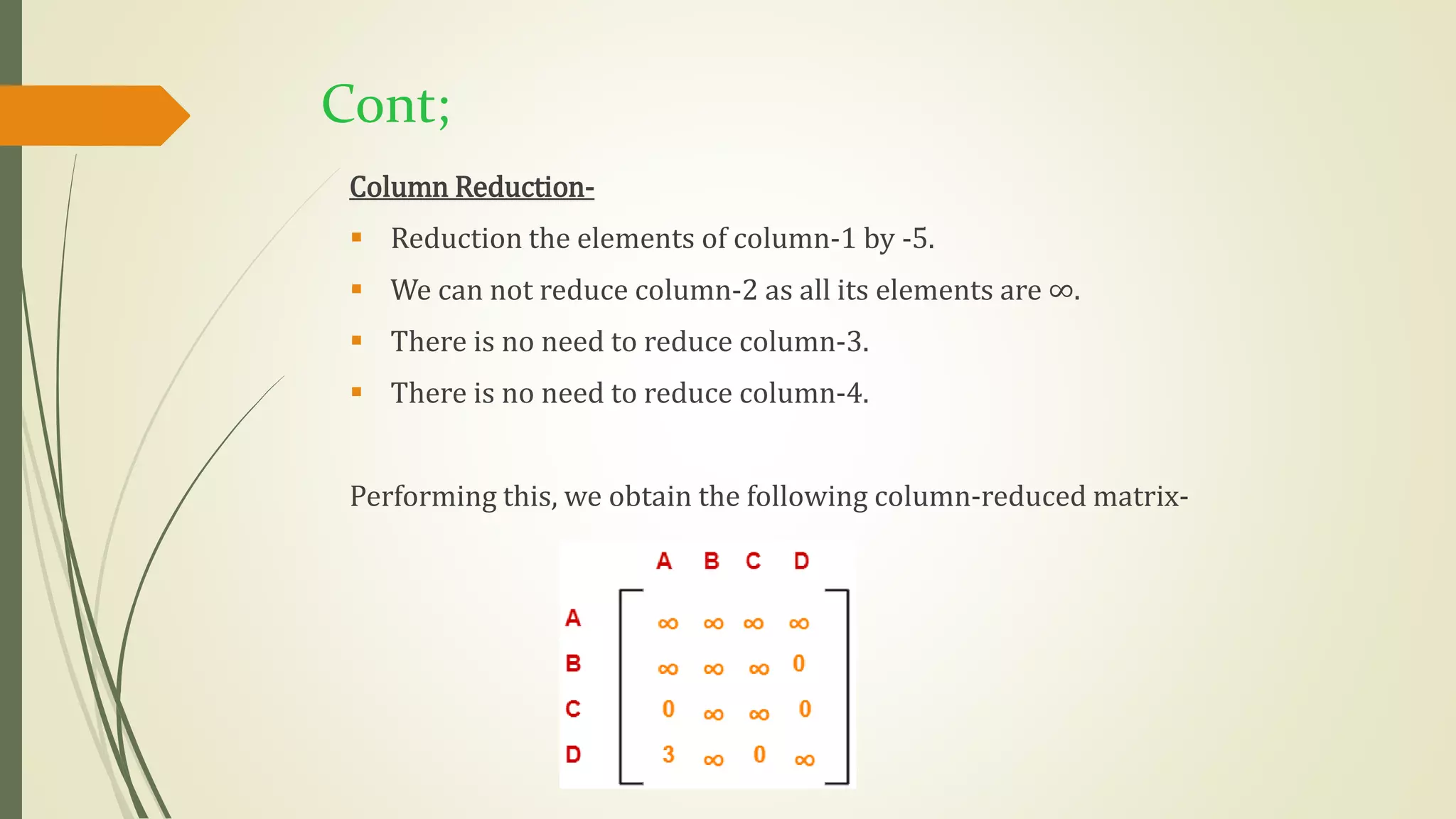
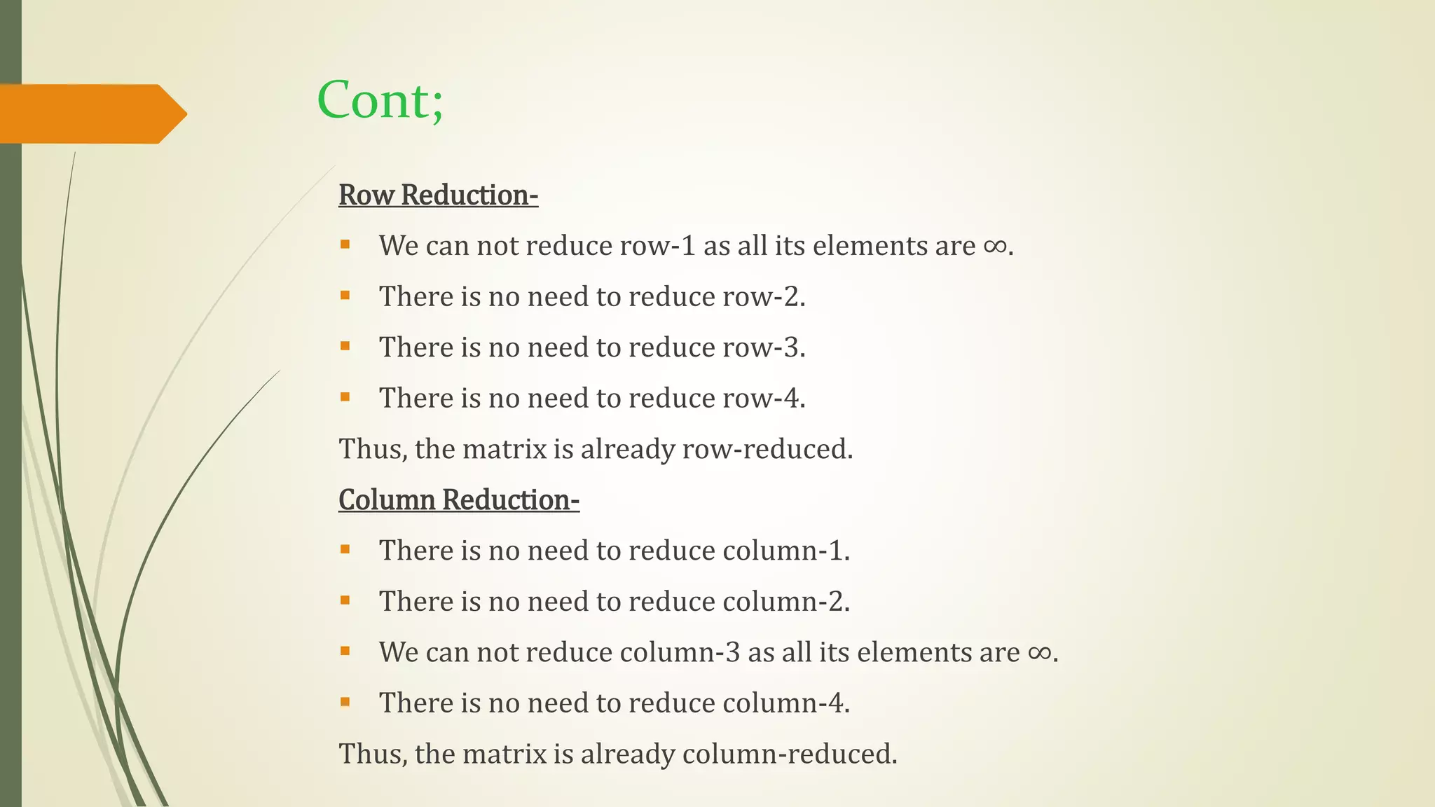
Column Reduction-
• There is no need to reduce column-1.
• There is no need to reduce column-2.
• There is no need to reduce column-3.
• We can not reduce column-4 as all its elements are ∞.
Thus, the matrix is already column-reduced.
Finally, the matrix is completely reduced.
Now, we calculate the cost of node-4.
Cost(4)
=Cost(1) + Sum of reduction elements + M[A,D]
=18 + 5 + 3
=26](https://image.slidesharecdn.com/datastructuresandalgorithms-220121073713/75/Data-structures-and-algorithms-21-2048.jpg)
![Cont;
Choosing To Go To Vertex-B: Node-5 (Path A C B)
• From the reduce matrix of step-02,M[C,B] = ∞.
• Set row-C and column-B to ∞.
• Set M[B,A] = ∞.
Now, resulting cost matrix is-](https://image.slidesharecdn.com/datastructuresandalgorithms-220121073713/75/Data-structures-and-algorithms-24-2048.jpg)
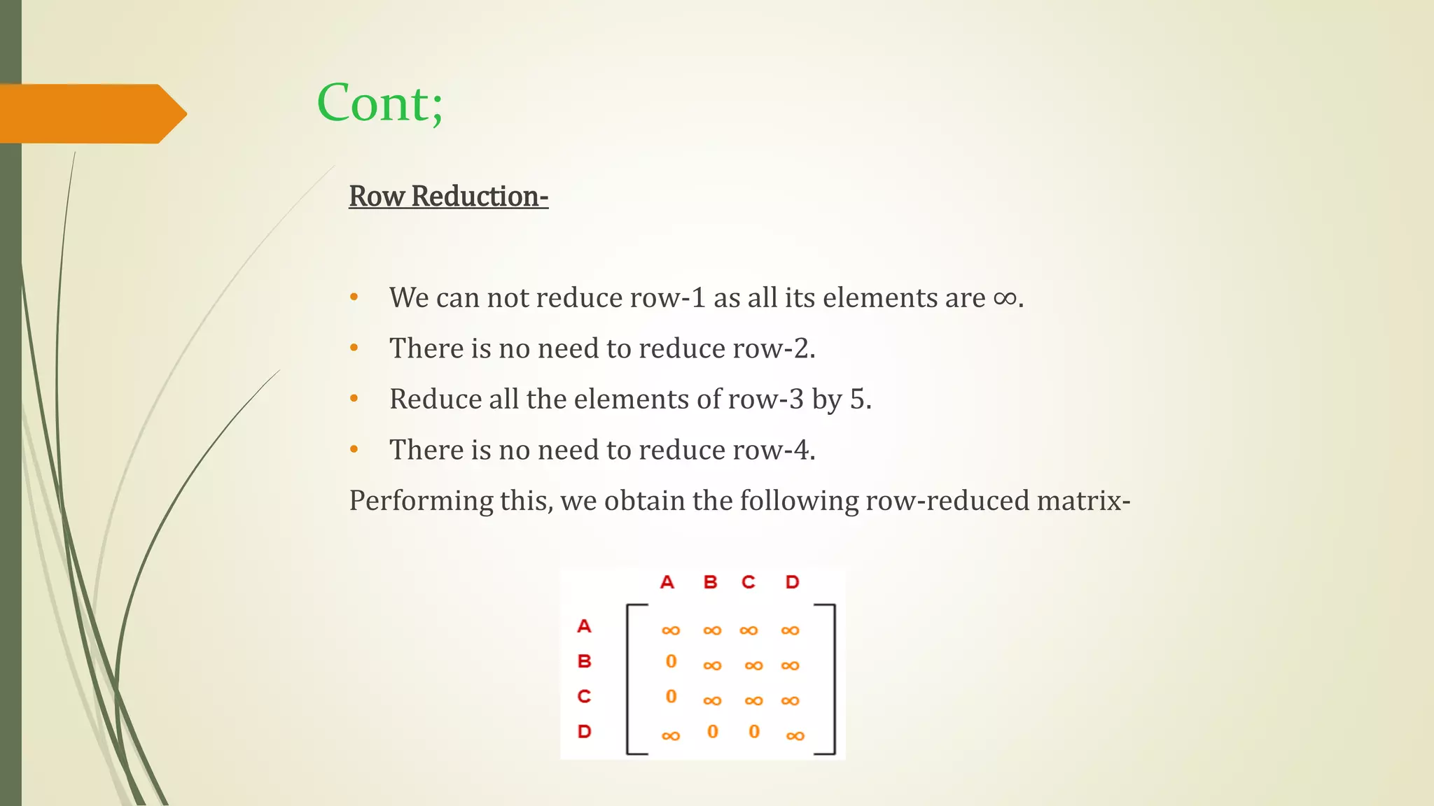
![Cont;
• There is no need to reduce column-4.
Thus, the matrix is already column reduced.
Finally, the matrix is completely reduced.
Now, we calculate the cost of node-5.
Cost(5)
=cost(3) + Sum of reduction elements + M[C,B]
=25 + (13 + 8) + ∞
= ∞.](https://image.slidesharecdn.com/datastructuresandalgorithms-220121073713/75/Data-structures-and-algorithms-27-2048.jpg)
![Cont;
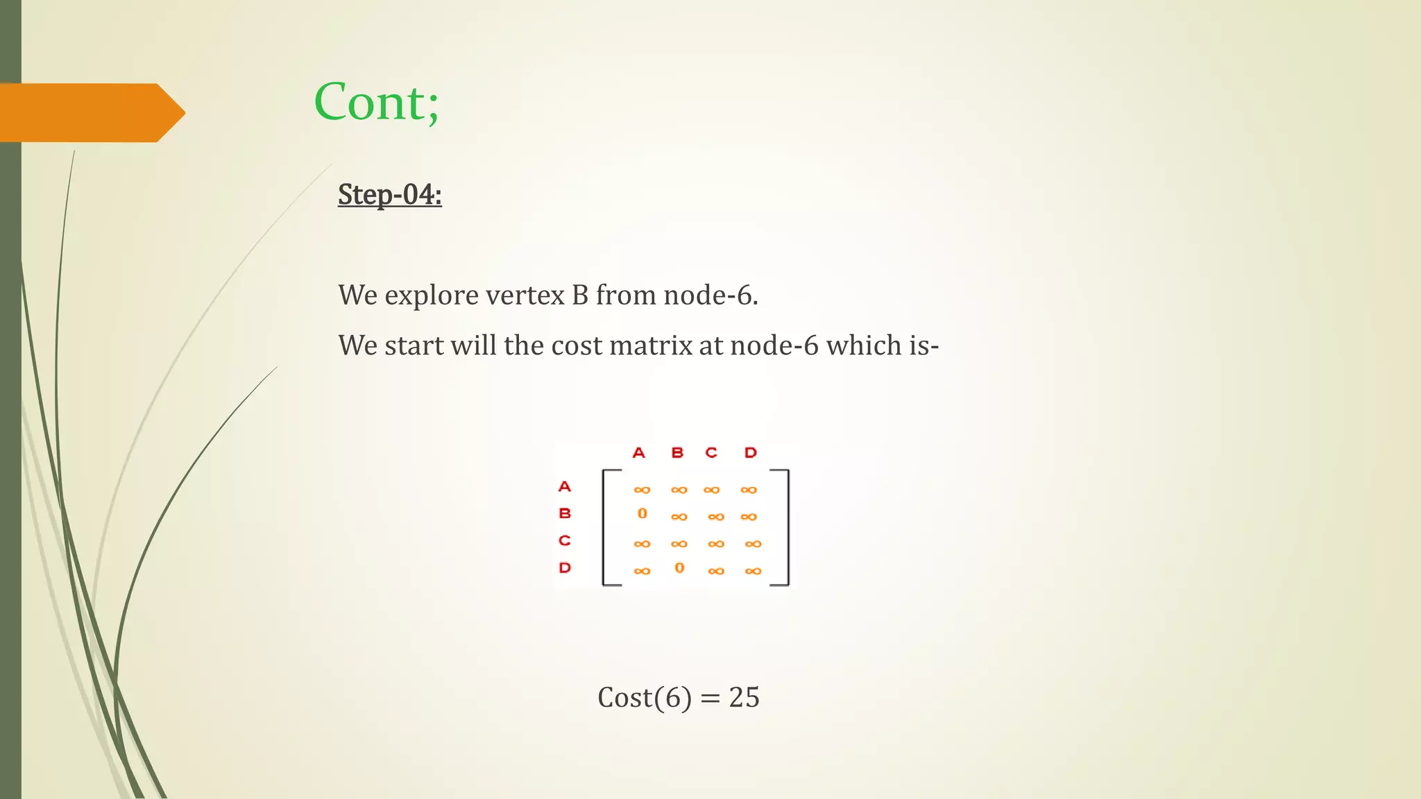
Choosing To Go To Vertex-D: Node-6 (Path A C D)
• From the reduced matrix of step-02,M[C,D] = ∞.
• Set row-C and column-D to ∞.
• Set M[D,A] = ∞.
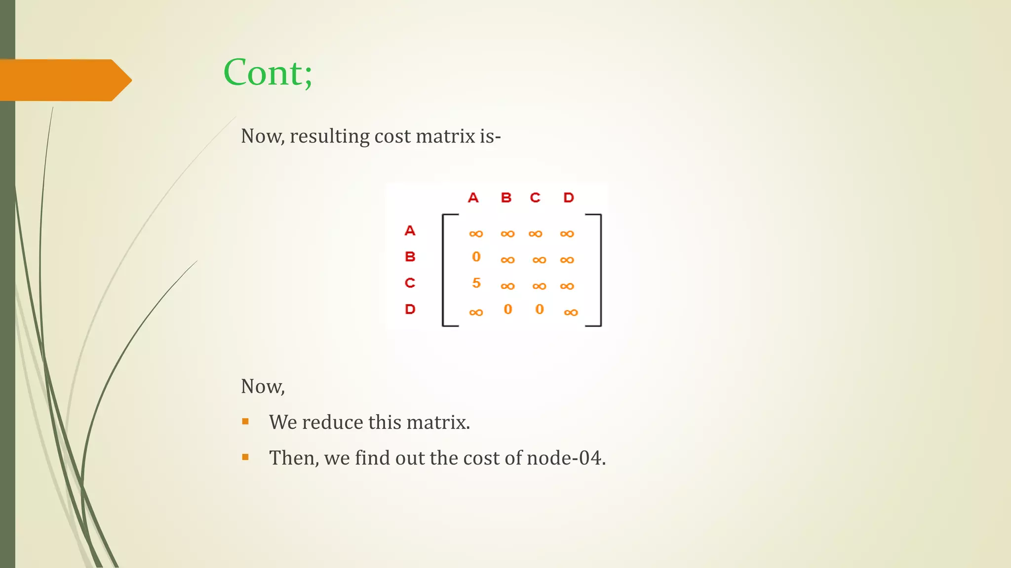
Now, resulting cost matrix is-](https://image.slidesharecdn.com/datastructuresandalgorithms-220121073713/75/Data-structures-and-algorithms-28-2048.jpg)
![Cont;
Cos(6)
=cost(3) + Sum of reduction elements + M[C,D]
=25 + 0 + 0
=25
Thus, we have-
Cost(5) = ∞ (for path A C B)
Cost(6) = 25 (for path A C D)
We choose the node with the lowest cost.
Since cost for node-6 is lowest, so we prefer to visit node-6.
Thus, we choose node-6 i.e, path C D](https://image.slidesharecdn.com/datastructuresandalgorithms-220121073713/75/Data-structures-and-algorithms-31-2048.jpg)
![Cont;
Choosing To Go To Vertex-B: Node-7 (Path A C D B)
• From the reduced matrix of step-03, M[D,B] = 0.
• Set row-D and column-B to ∞.
• Set M[B,A] = ∞.
Now, resulting cost matrix is-](https://image.slidesharecdn.com/datastructuresandalgorithms-220121073713/75/Data-structures-and-algorithms-33-2048.jpg)
![Cont;
Now, we calculate the cost node-7
Cost(7)
=cost(6) + Sum of reduction elements + M[D,B]
=25 + 0 + 0
=25
Thus,
Optimal path is: A C D B A
Cost of Optimal path is = 25 units.](https://image.slidesharecdn.com/datastructuresandalgorithms-220121073713/75/Data-structures-and-algorithms-36-2048.jpg)


![Cont;
Step-02:
o We consider all other vertices one by one.
o We select the best vertex where we can land upon to minimize the tour cost.
Choosing To Go To Vertex-B: Node-2(Path A B)
• From the reduced matrix of step-1, M[A,B] = 0
• Set row-A and column-B to ∞
• Set M[B,A] = ∞](https://crownmelresort.com/image.slidesharecdn.com/datastructuresandalgorithms-220121073713/75/Data-structures-and-algorithms-11-2048.jpg)


![Cont;
Finally, the matrix is completely reduced.
Now, we calculate the cost of node-2.
Cost(2)
=Cost(1) + Sum of reduction elements + M[A,B]
=18 + (13 + 5) +0
=36
Choosing To Go To Vertex-C: Node-3 (Path A C)
From the reduced matrix of step-01,M[A,C]=7
Set row-A and column-C to ∞.
Set M[C,A] = ∞.](https://crownmelresort.com/image.slidesharecdn.com/datastructuresandalgorithms-220121073713/75/Data-structures-and-algorithms-15-2048.jpg)


![Cont;
Finally, the matrix is completely reduced.
Now, we calculate the cost of node-3.
Cost(3)
=Cost(1) + Sum of reduction elements + M[A,C]
=18 + 0 + 7
=25
Choosing To Go To Vertex-D: Node-4 (Path A D)
• From the reduced matrix of step-01,M[A,D] = 3
• Set row-A and column-D to ∞.
• Set M[D,A] = ∞.](https://crownmelresort.com/image.slidesharecdn.com/datastructuresandalgorithms-220121073713/75/Data-structures-and-algorithms-18-2048.jpg)


![Cont;
Column Reduction-
• There is no need to reduce column-1.
• There is no need to reduce column-2.
• There is no need to reduce column-3.
• We can not reduce column-4 as all its elements are ∞.
Thus, the matrix is already column-reduced.
Finally, the matrix is completely reduced.
Now, we calculate the cost of node-4.
Cost(4)
=Cost(1) + Sum of reduction elements + M[A,D]
=18 + 5 + 3
=26](https://crownmelresort.com/image.slidesharecdn.com/datastructuresandalgorithms-220121073713/75/Data-structures-and-algorithms-21-2048.jpg)


![Cont;
Choosing To Go To Vertex-B: Node-5 (Path A C B)
• From the reduce matrix of step-02,M[C,B] = ∞.
• Set row-C and column-B to ∞.
• Set M[B,A] = ∞.
Now, resulting cost matrix is-](https://crownmelresort.com/image.slidesharecdn.com/datastructuresandalgorithms-220121073713/75/Data-structures-and-algorithms-24-2048.jpg)


![Cont;
• There is no need to reduce column-4.
Thus, the matrix is already column reduced.
Finally, the matrix is completely reduced.
Now, we calculate the cost of node-5.
Cost(5)
=cost(3) + Sum of reduction elements + M[C,B]
=25 + (13 + 8) + ∞
= ∞.](https://crownmelresort.com/image.slidesharecdn.com/datastructuresandalgorithms-220121073713/75/Data-structures-and-algorithms-27-2048.jpg)
![Cont;
Choosing To Go To Vertex-D: Node-6 (Path A C D)
• From the reduced matrix of step-02,M[C,D] = ∞.
• Set row-C and column-D to ∞.
• Set M[D,A] = ∞.
Now, resulting cost matrix is-](https://crownmelresort.com/image.slidesharecdn.com/datastructuresandalgorithms-220121073713/75/Data-structures-and-algorithms-28-2048.jpg)


![Cont;
Cos(6)
=cost(3) + Sum of reduction elements + M[C,D]
=25 + 0 + 0
=25
Thus, we have-
Cost(5) = ∞ (for path A C B)
Cost(6) = 25 (for path A C D)
We choose the node with the lowest cost.
Since cost for node-6 is lowest, so we prefer to visit node-6.
Thus, we choose node-6 i.e, path C D](https://crownmelresort.com/image.slidesharecdn.com/datastructuresandalgorithms-220121073713/75/Data-structures-and-algorithms-31-2048.jpg)

![Cont;
Choosing To Go To Vertex-B: Node-7 (Path A C D B)
• From the reduced matrix of step-03, M[D,B] = 0.
• Set row-D and column-B to ∞.
• Set M[B,A] = ∞.
Now, resulting cost matrix is-](https://crownmelresort.com/image.slidesharecdn.com/datastructuresandalgorithms-220121073713/75/Data-structures-and-algorithms-33-2048.jpg)


![Cont;
Now, we calculate the cost node-7
Cost(7)
=cost(6) + Sum of reduction elements + M[D,B]
=25 + 0 + 0
=25
Thus,
Optimal path is: A C D B A
Cost of Optimal path is = 25 units.](https://crownmelresort.com/image.slidesharecdn.com/datastructuresandalgorithms-220121073713/75/Data-structures-and-algorithms-36-2048.jpg)