2
The personnel assignment
problem
Alinearly ordered set of persons P={P1
, P2
, …, P
n
} where P1
<P2
<…<Pn
A partially ordered set of jobs J={J1
, J2
, …, Jn
}
Suppose that Pi
and Pj
are assigned to jobs f(Pi
) a
nd f(Pj
) respectively. If f(Pi
) f(Pj
), then Pi
Pj
. C
ost Cij
is the cost of assigning Pi
to Jj
. We want to
find a feasible assignment with the min. cost. i.e.
Minimize i,j
Cij
Xij
,
where Xij
= 1 if Pi
is assigned to Jj
and Xij
= 0 othe
rwise.
3.
3
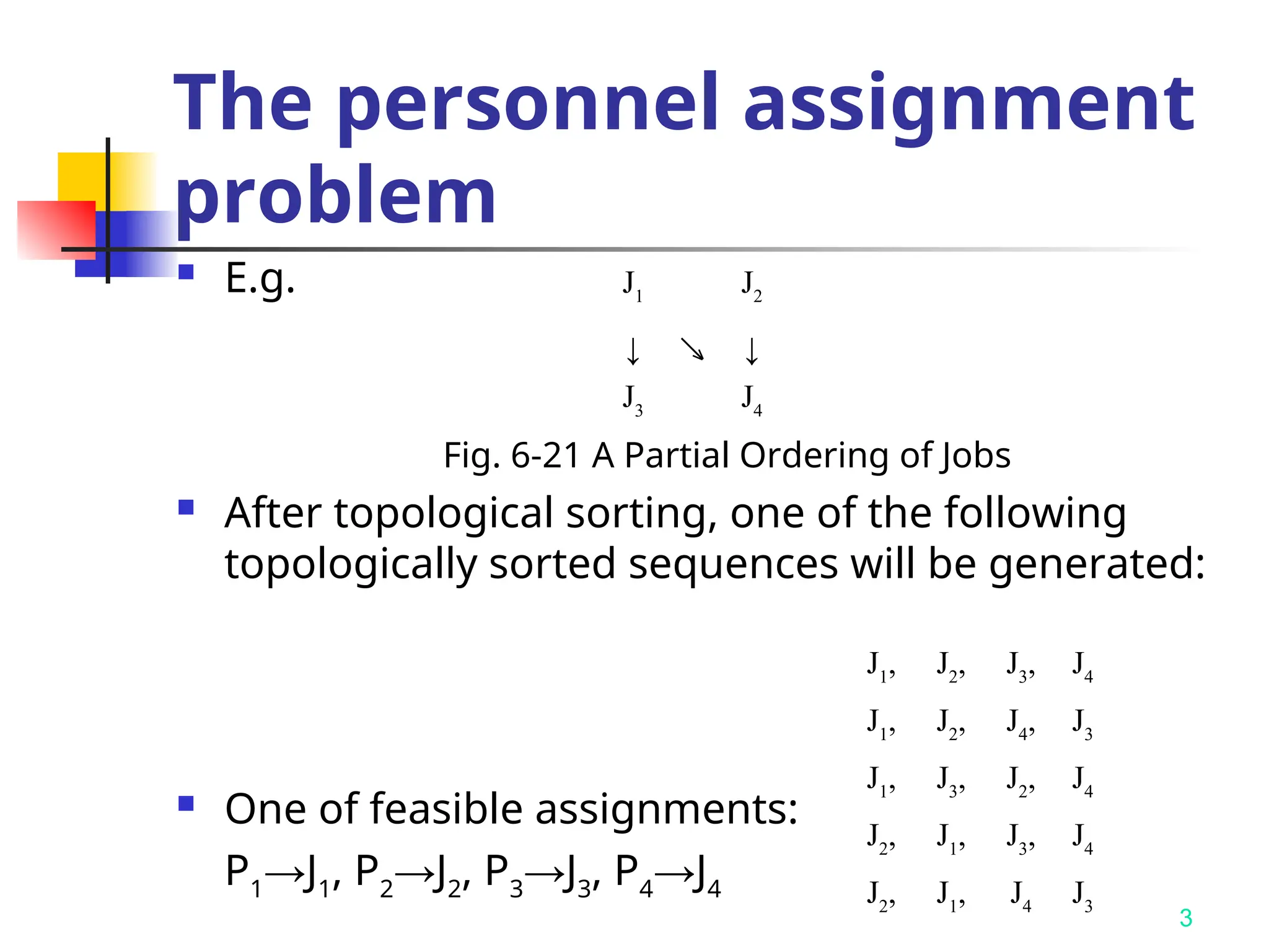
E.g.
Fig. 6-21A Partial Ordering of Jobs
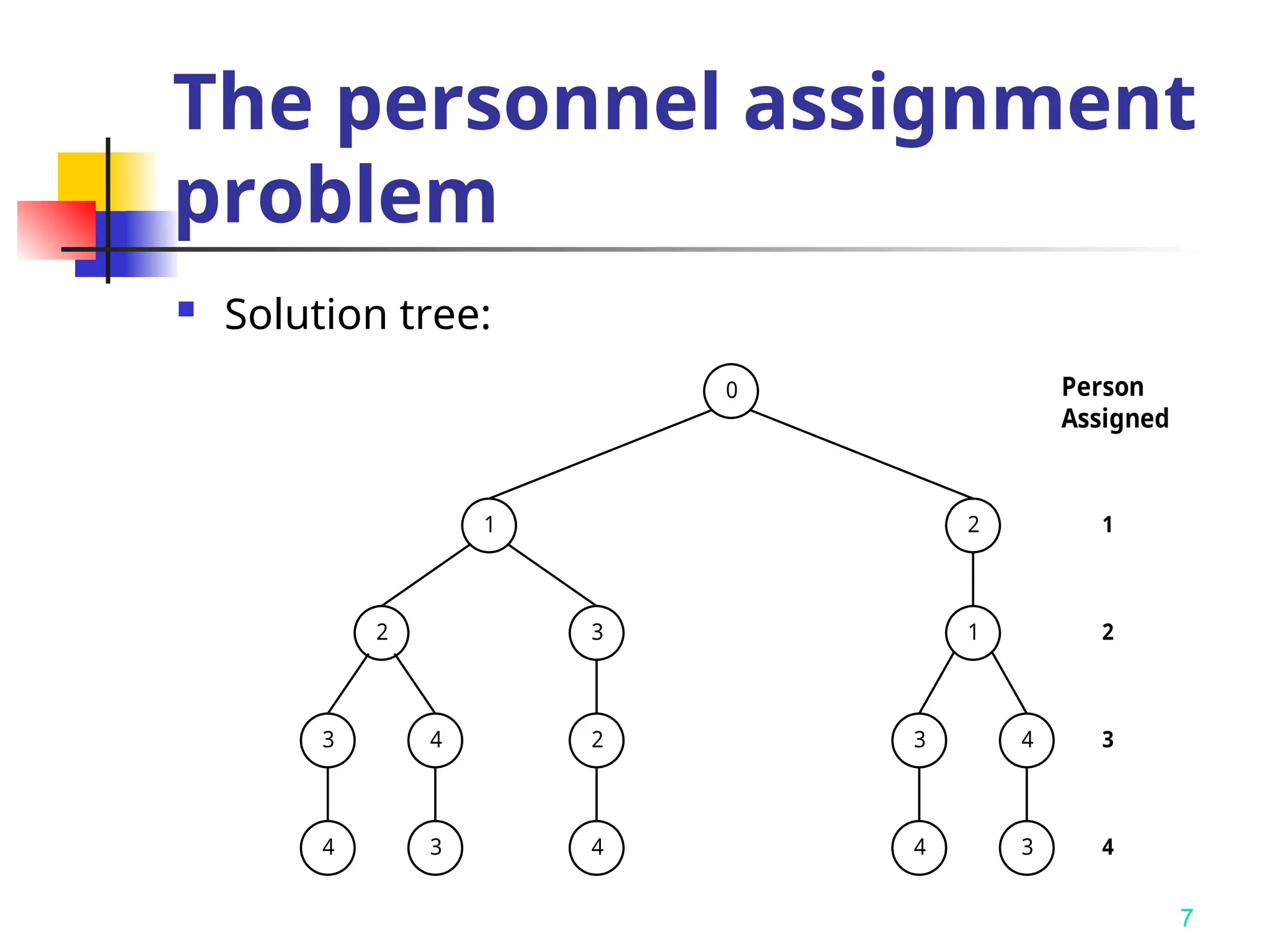
After topological sorting, one of the following
topologically sorted sequences will be generated:
One of feasible assignments:
P1
→J1
, P2
→J2
, P3
→J3
, P4
→J4
J1
J2
↓ ↘ ↓
J3
J4
J1
, J2
, J3
, J4
J1
, J2
, J4
, J3
J1
, J3
, J2
, J4
J2
, J1
, J3
, J4
J2
, J1
, J4
J3
The personnel assignment
problem
4.
4
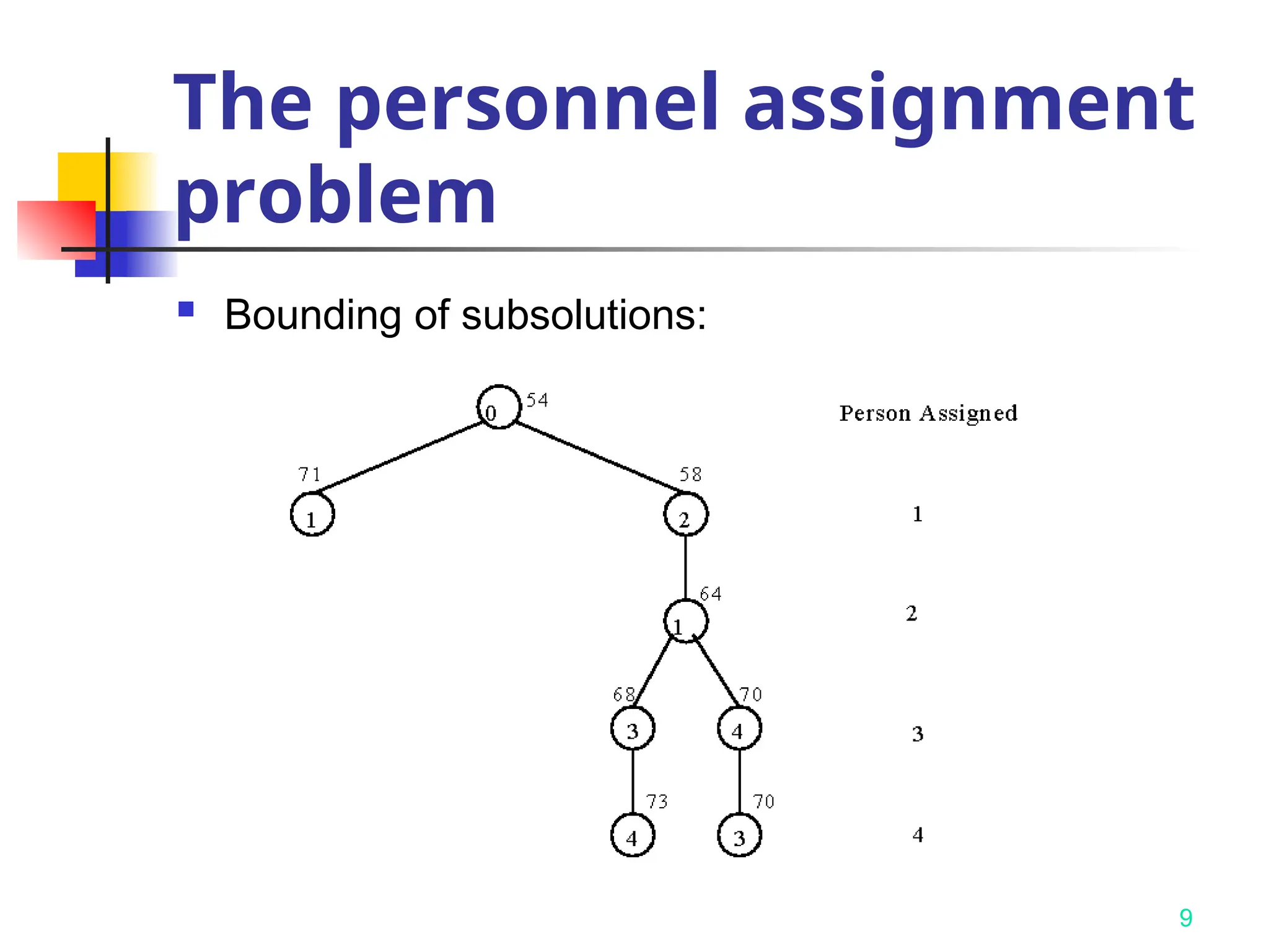
The personnel assignment
problem
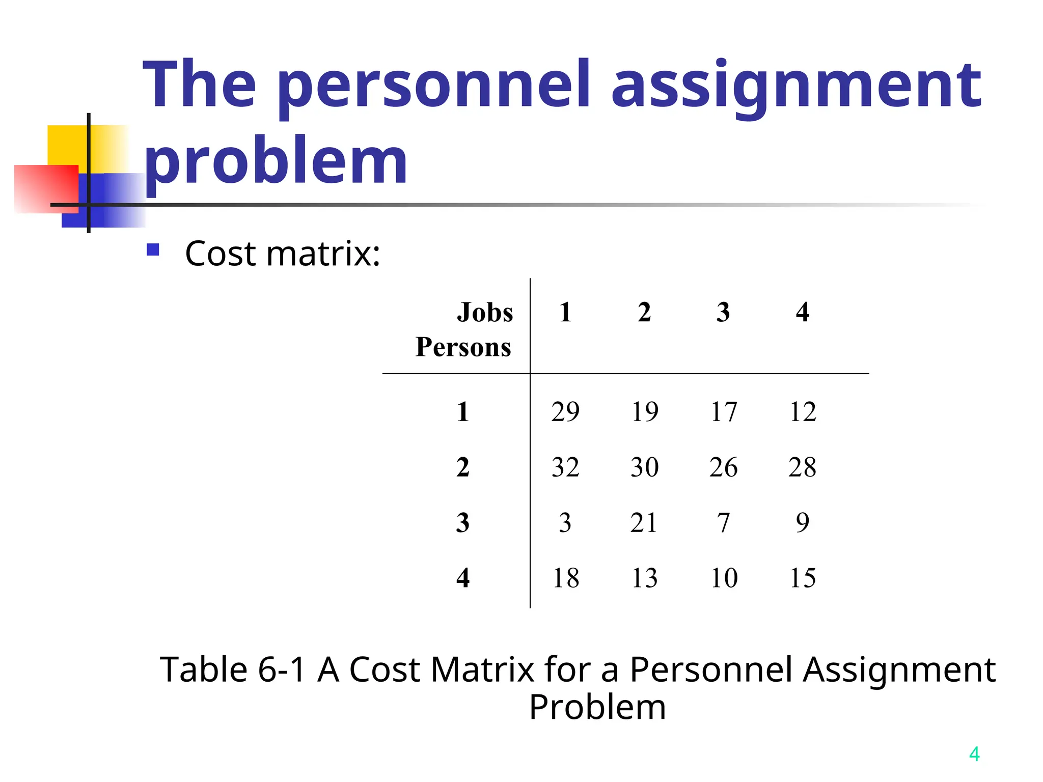
Cost matrix:
Table 6-1 A Cost Matrix for a Personnel Assignment
Problem
Jobs
Persons
1 2 3 4
1 29 19 17 12
2 32 30 26 28
3 3 21 7 9
4 18 13 10 15
5.
5
The personnel assignment
problem
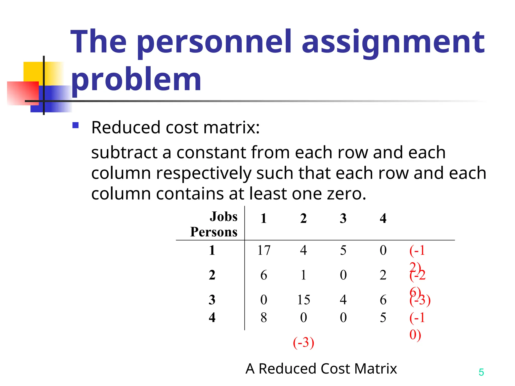
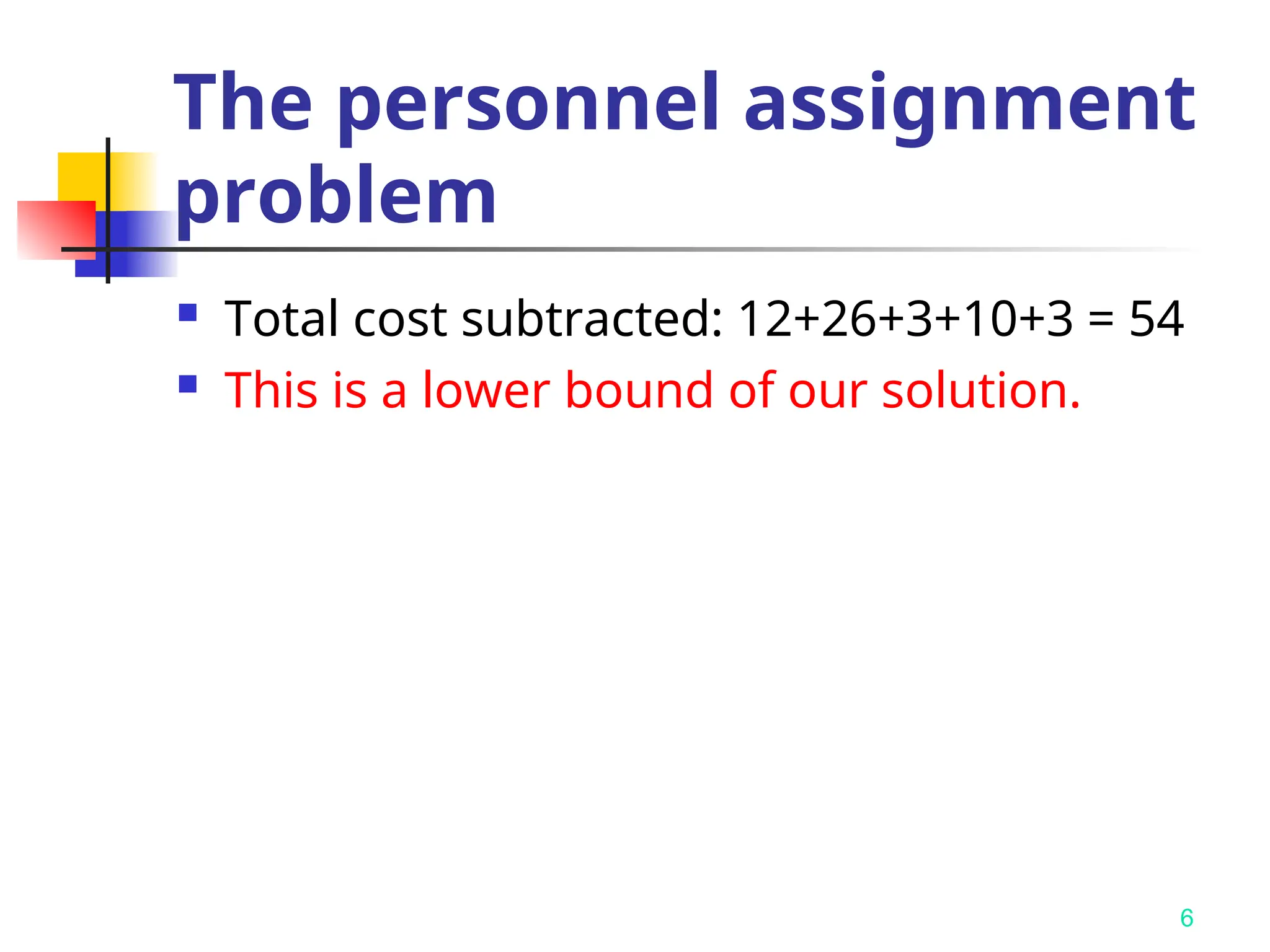
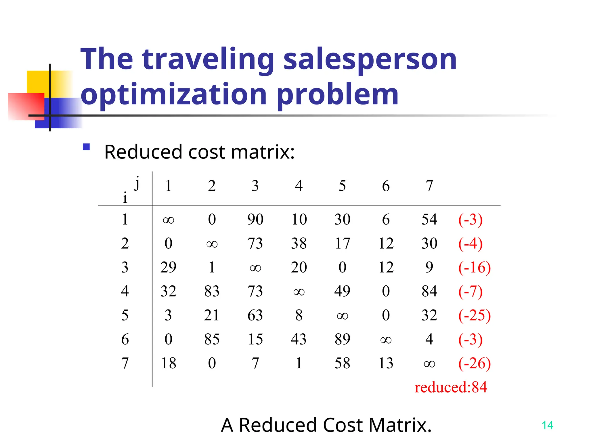
Reduced cost matrix:
subtract a constant from each row and each
column respectively such that each row and each
column contains at least one zero.
A Reduced Cost Matrix
Jobs
Persons
1 2 3 4
1 17 4 5 0 (-1
2)
2 6 1 0 2 (-2
6)
3 0 15 4 6 (-3)
4 8 0 0 5 (-1
0)
(-3)
8
Steps to generatesolution tress
Step 1: Add the original partial ordering into stack.
Step 2: Remove the top partial ordering O from st
ack. If O contains only one element E, then stop
(with the element E being an element in the topolo
gically sorted sequence). Otherwise, add the parti
al orderings into the stack each of which is derived
by removing an element E not preceded by any ot
her element in the partial ordering O. (Every E is a
n element in the topologically sorted sequence.)
Step 3: Goto Step 1.
10
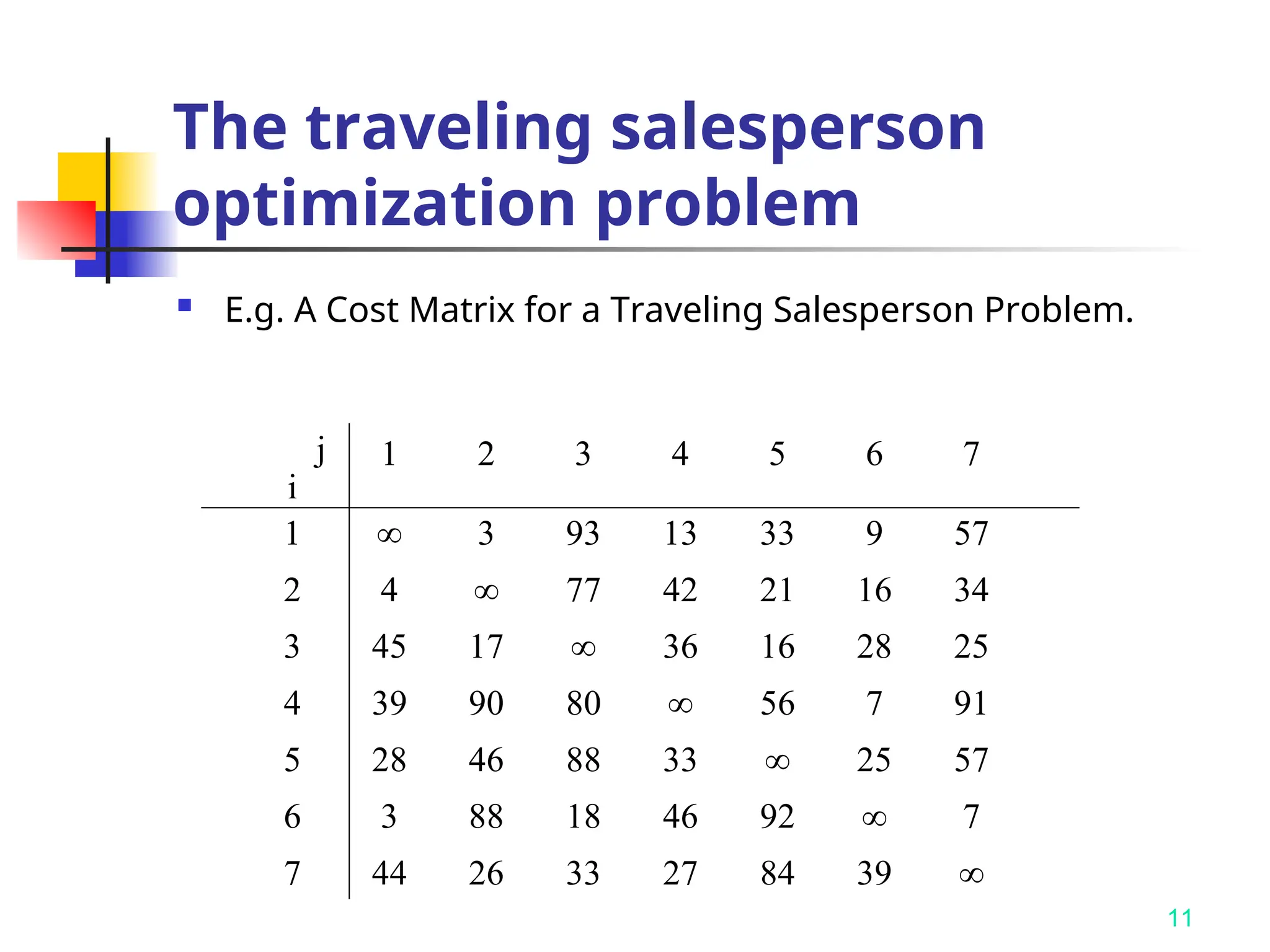
The traveling salesperson
optimizationproblem
Given a graph, the TSP Optimization
problem is to find a tour, starting
from any vertex, visiting every other
vertex and returning to the starting
vertex, with minimal cost.
It is NP-complete
We try to avoid n! exhaustive search
by the branch-and-bound technique.
12
The basic idea
There is a way to split the solution space
(branch)
There is a way to predict a lower bound for
a class of solutions. There is also a way to
find a upper bound of an optimal solution.
If the lower bound of a solution exceeds
the upper bound, this solution cannot be
optimal and thus we should terminate the
branching associated with this solution.
13.
13
Splitting
We splita solution into two groups:
One group including a particular arc
The other excluding the arc
Each splitting incurs a lower bound
and we shall traverse the searching
tree with the “lower” lower bound.
16
Lower bound
Thetotal cost of 84+12=96 is
subtracted. Thus, we know the lower
bound of this TSP problem is 96.
17.
17
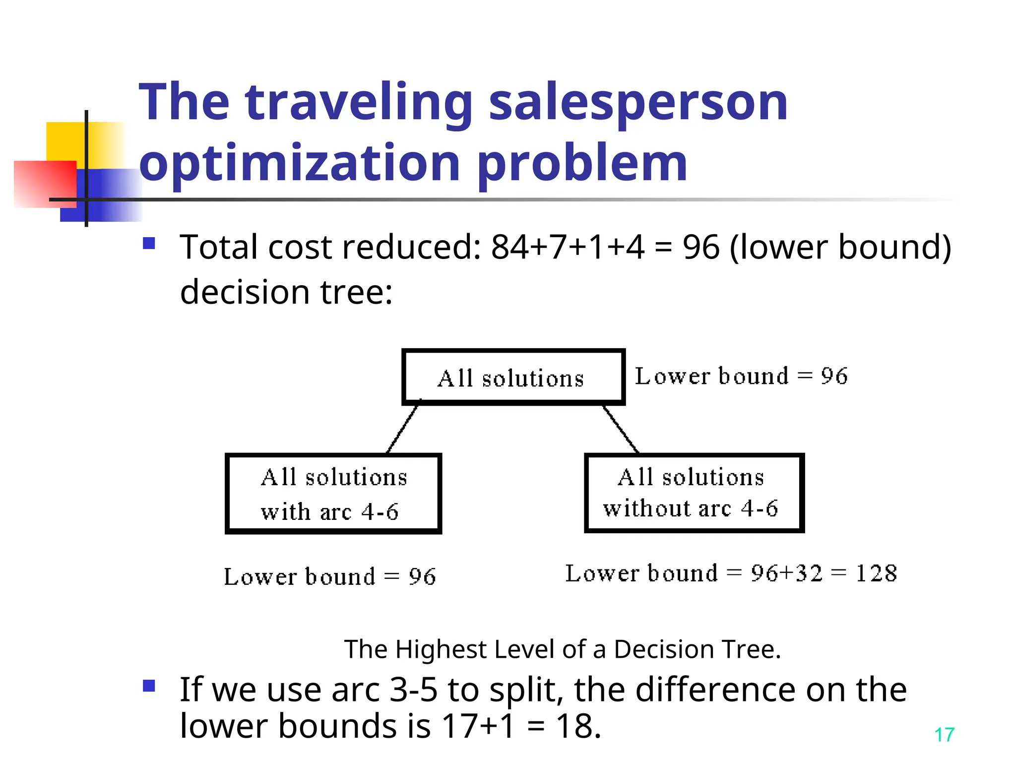
Total costreduced: 84+7+1+4 = 96 (lower bound)
decision tree:
The Highest Level of a Decision Tree.
If we use arc 3-5 to split, the difference on the
lower bounds is 17+1 = 18.
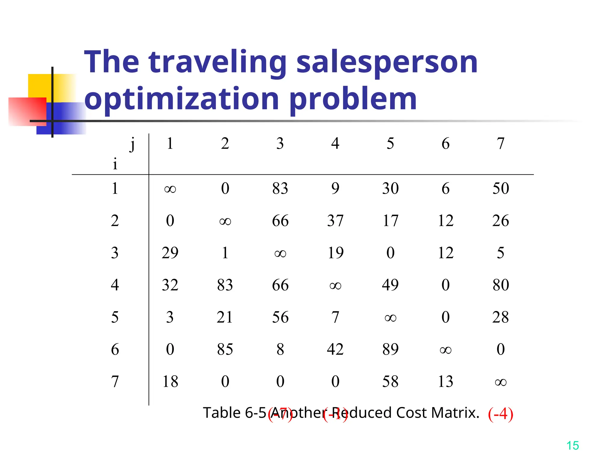
The traveling salesperson
optimization problem
18.
18
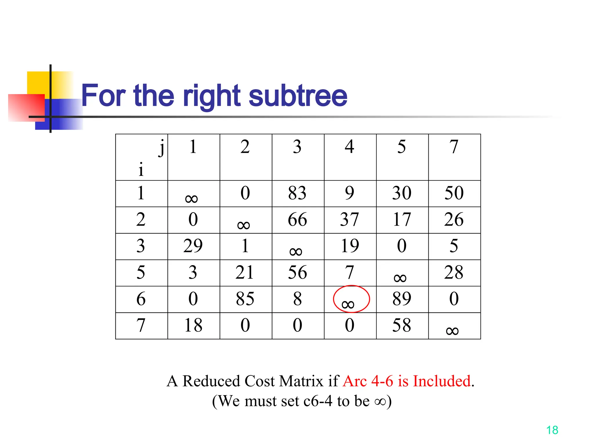
For the rightsubtree
j
i
1 2 3 4 5 7
1 ∞ 0 83 9 30 50
2 0 ∞ 66 37 17 26
3 29 1 ∞ 19 0 5
5 3 21 56 7 ∞ 28
6 0 85 8 ∞ 89 0
7 18 0 0 0 58 ∞
A Reduced Cost Matrix if Arc 4-6 is Included.
(We must set c6-4 to be )
19.
19
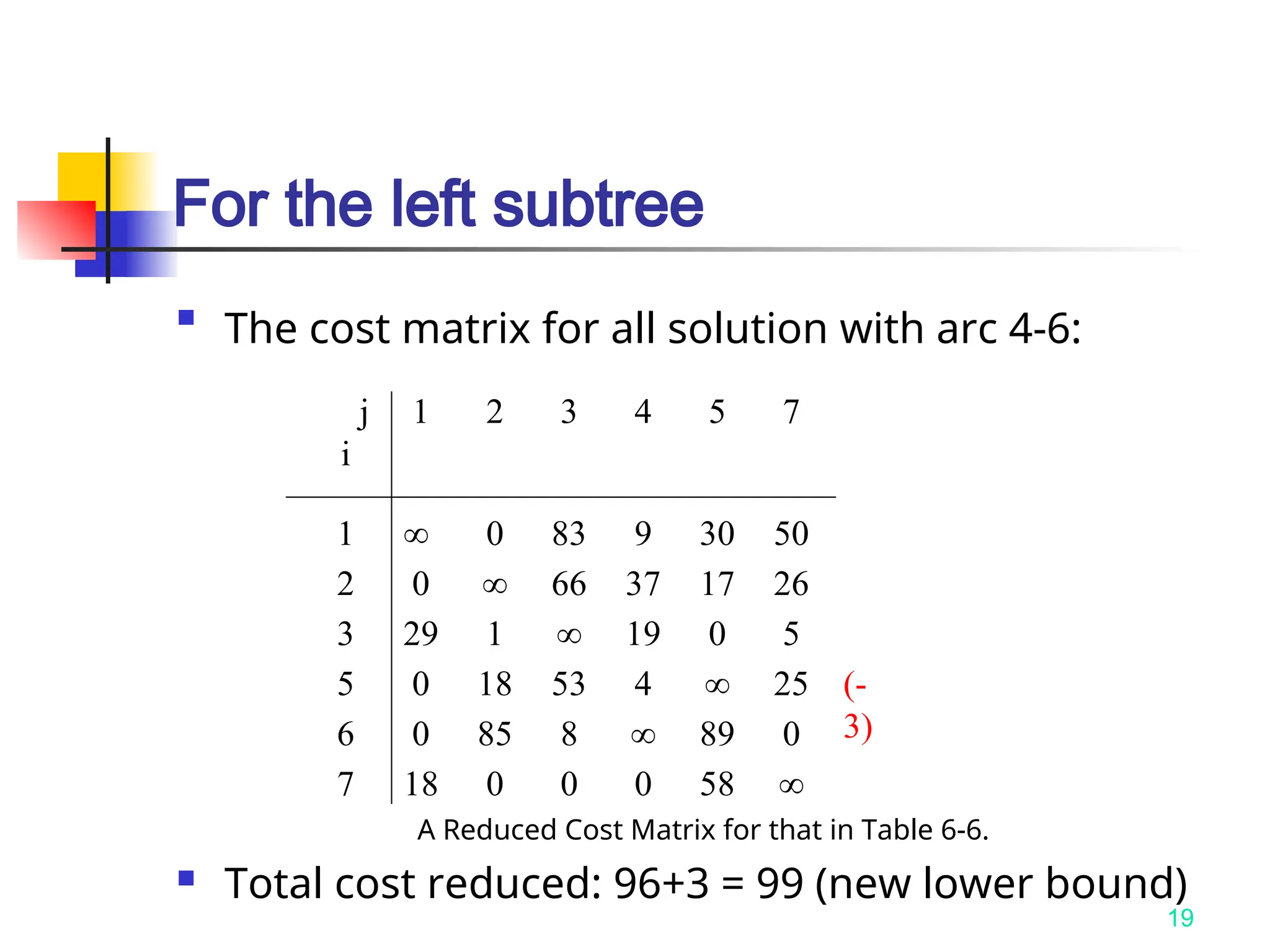
For the leftsubtree
The cost matrix for all solution with arc 4-6:
A Reduced Cost Matrix for that in Table 6-6.
Total cost reduced: 96+3 = 99 (new lower bound)
j
i
1 2 3 4 5 7
1 ∞ 0 83 9 30 50
2 0 ∞ 66 37 17 26
3 29 1 ∞ 19 0 5
5 0 18 53 4 ∞ 25 (-
3)
6 0 85 8 ∞ 89 0
7 18 0 0 0 58 ∞
20.
20
Upper bound
Wefollow the best-first search scheme
and can obtain a feasible solution with c
ost C.
C serves as an upper bound and many
branchings may be terminated if their lo
wer bounds exceed C.
21.
21
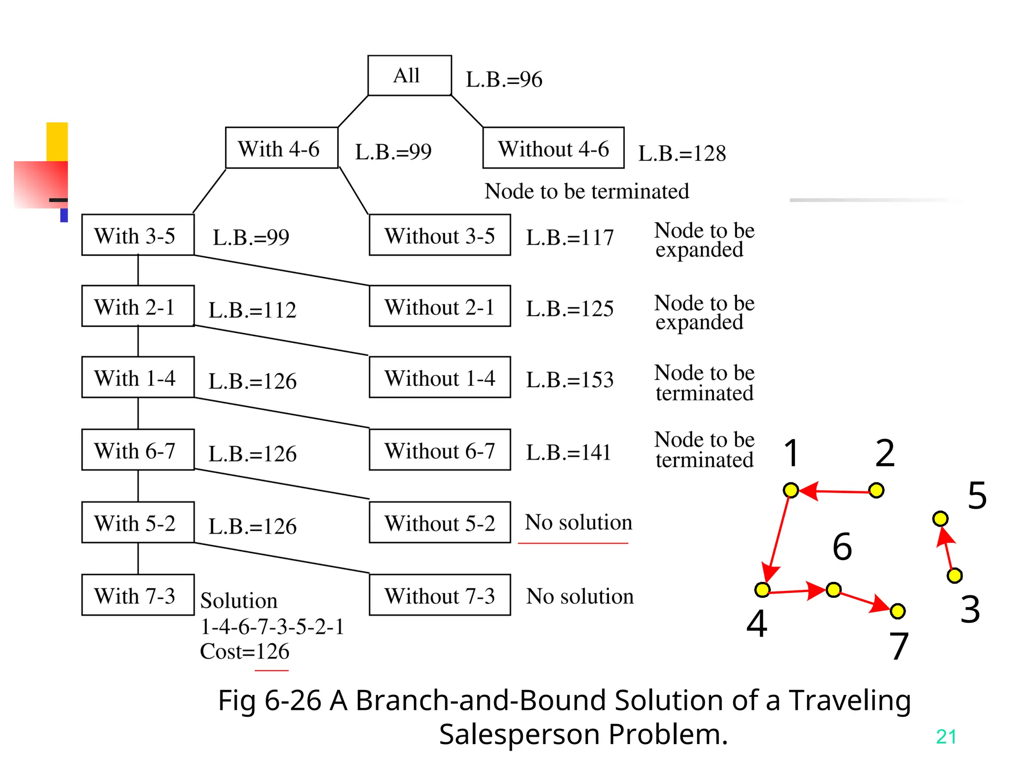
Fig 6-26 ABranch-and-Bound Solution of a Traveling
Salesperson Problem.
1 2
3
5
6
7
4
22.
22
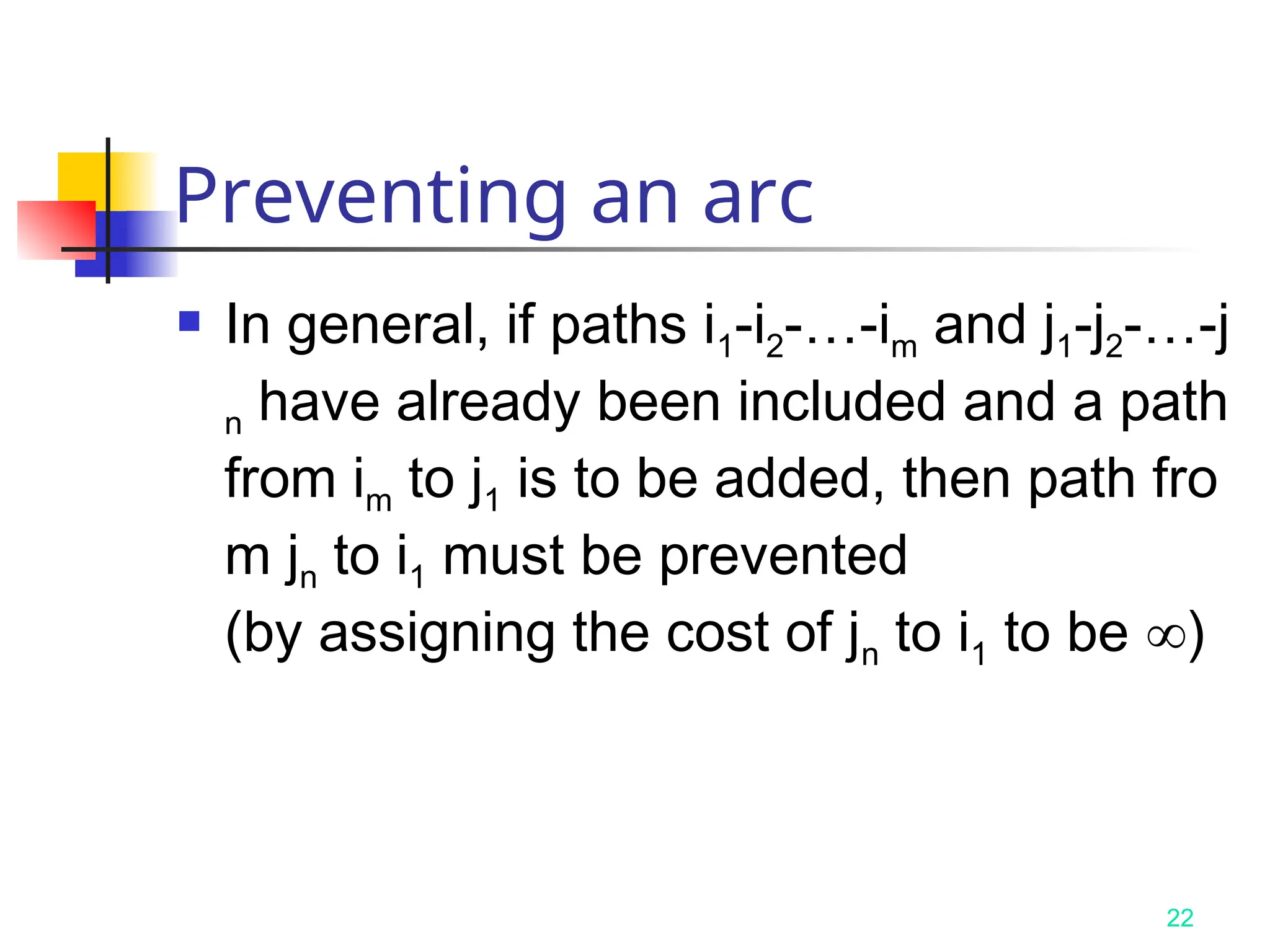
Preventing an arc
In general, if paths i1-i2-…-im and j1-j2-…-j
n have already been included and a path
from im to j1 is to be added, then path fro
m jn to i1 must be prevented
(by assigning the cost of jn to i1 to be )
23.
23
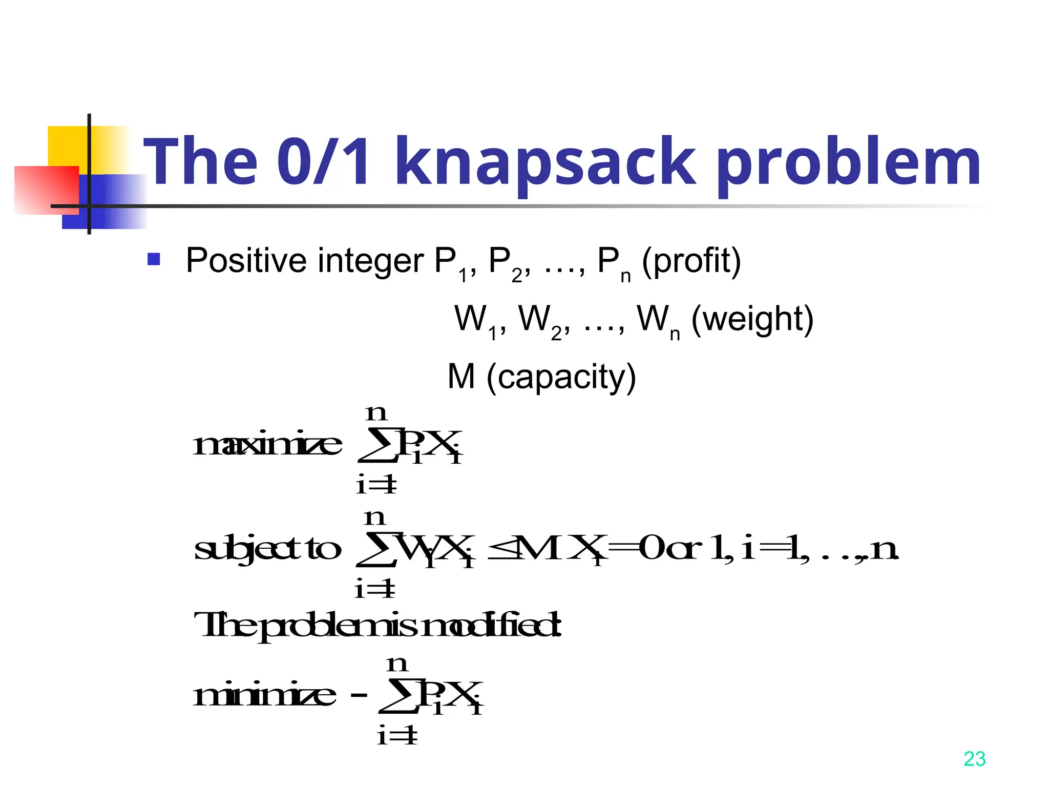
The 0/1 knapsackproblem
Positive integer P1
, P2
, …, Pn
(profit)
W1
, W2
, …, Wn
(weight)
M (capacity)
m
a
x
im
iz
e PX
i i
i
n
1
s
u
b
je
c
tto W
X M
i i
i
n
1
X
i =0o
r1
,i=
1
,…
,n
.
T
h
ep
r
o
b
le
m
ism
o
d
if
ie
d
:
m
in
im
iz
e
PX
i i
i
n
1
24.
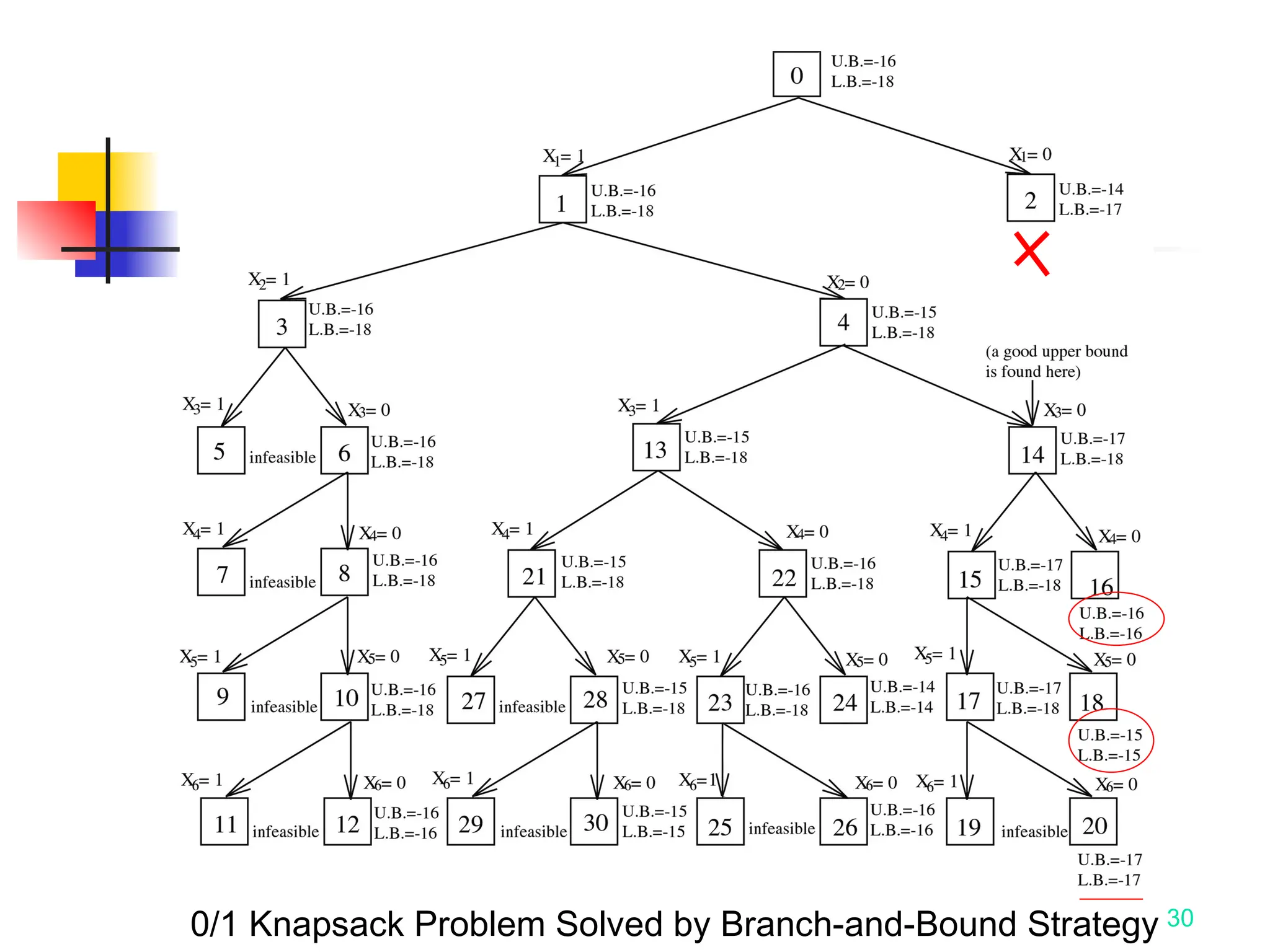
24
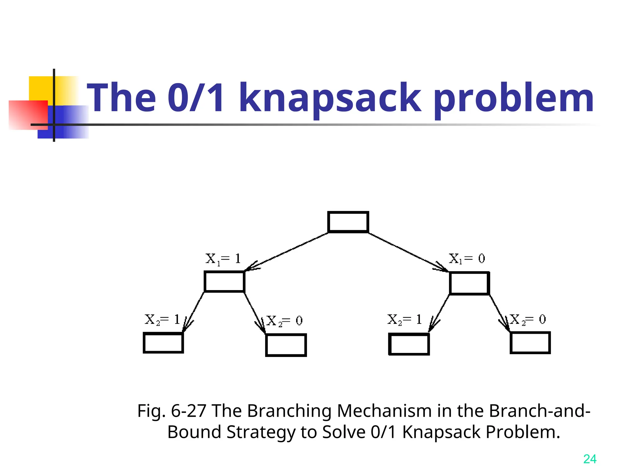
The 0/1 knapsackproblem
Fig. 6-27 The Branching Mechanism in the Branch-and-
Bound Strategy to Solve 0/1 Knapsack Problem.
25.
25
How to findthe upper
bound?
Ans: by quickly finding a feasible solutio
n: starting from the smallest available i,
scanning towards the largest i’s until M i
s exceeded. The upper bound can be c
alculated.
26.
26
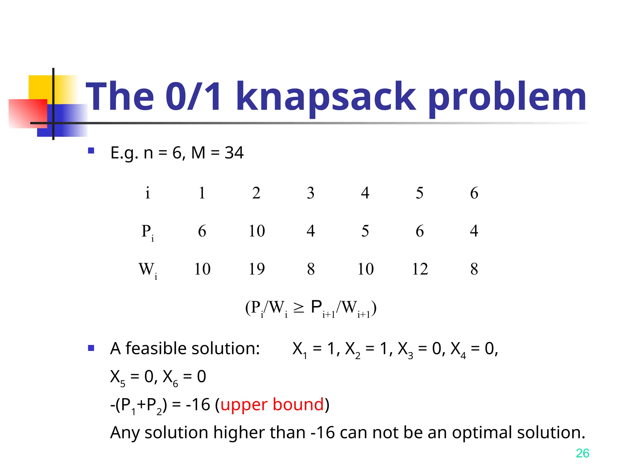
The 0/1 knapsackproblem
E.g. n = 6, M = 34
A feasible solution: X1
= 1, X2
= 1, X3
= 0, X4
= 0,
X5
= 0, X6
= 0
-(P1
+P2
) = -16 (upper bound)
Any solution higher than -16 can not be an optimal solution.
i 1 2 3 4 5 6
Pi
6 10 4 5 6 4
Wi
10 19 8 10 12 8
(Pi
/Wi
Pi+1
/Wi+1
)
27.
27
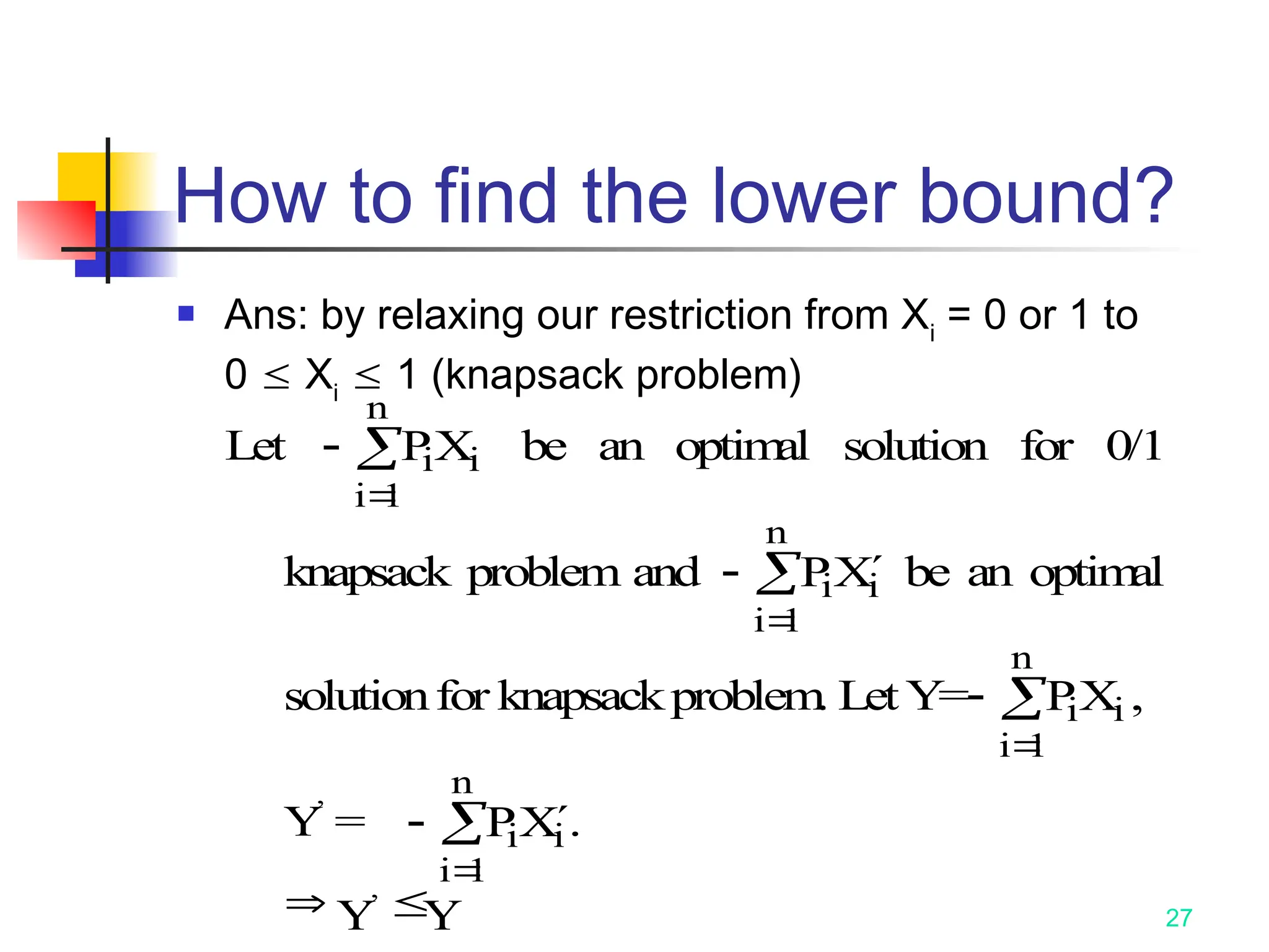
How to findthe lower bound?
Ans: by relaxing our restriction from Xi
= 0 or 1 to
0 Xi
1 (knapsack problem)
Let
PX
i i
i
n
1
be an optim
al solution for 0/1
knapsack problem and
PX
i
i
n
i
1
be an optim
al
solutionfor knapsackproblem
. LetY=
PX
i i
i
n
1
,
Y’
=
PX
i
i
n
i
1
.
Y’
Y
28.
28
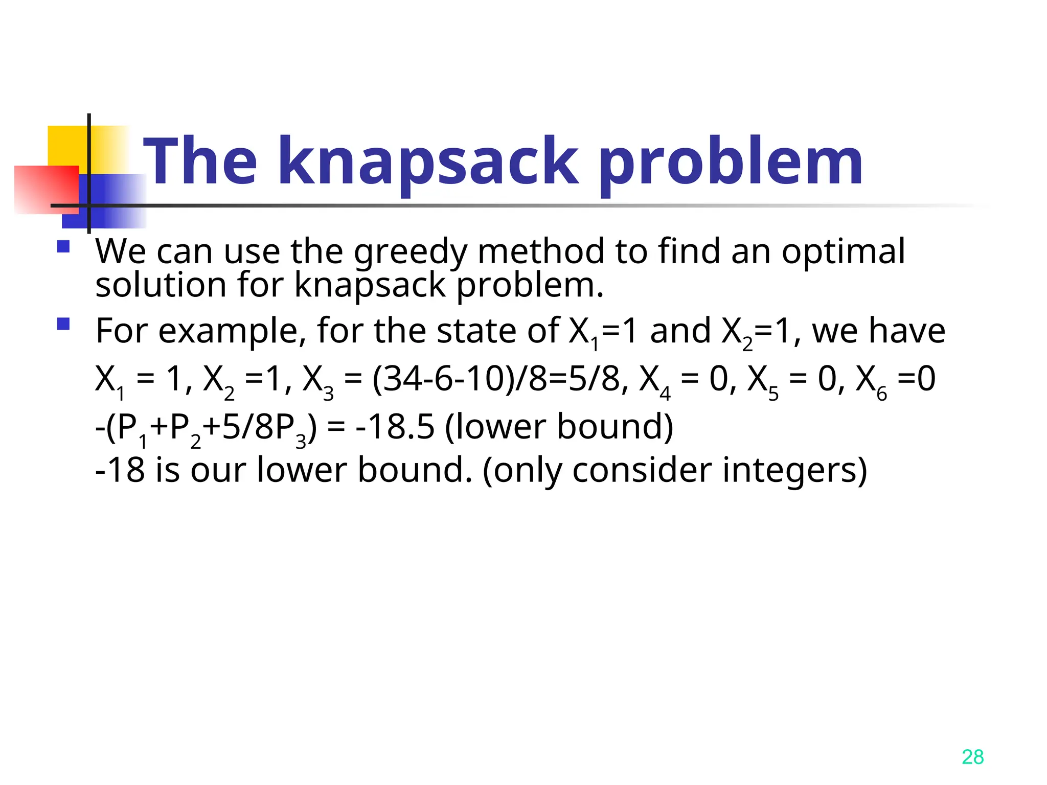
The knapsack problem
We can use the greedy method to find an optimal
solution for knapsack problem.
For example, for the state of X1=1 and X2=1, we have
X1
= 1, X2
=1, X3
= (34-6-10)/8=5/8, X4
= 0, X5
= 0, X6
=0
-(P1
+P2
+5/8P3
) = -18.5 (lower bound)
-18 is our lower bound. (only consider integers)
29.
29
How to expandthe tree?
By the best-first search scheme
That is, by expanding the node with
the best lower bound. If two nodes
have the same lower bounds, expand
the node with the lower upper
bound.
31
Node 2is terminated because its lower
bound is equal to the upper bound of
node 14.
Nodes 16, 18 and others are terminated
because the local lower bound is equal
to the local upper bound.
(lower bound optimal solution
upper bound)
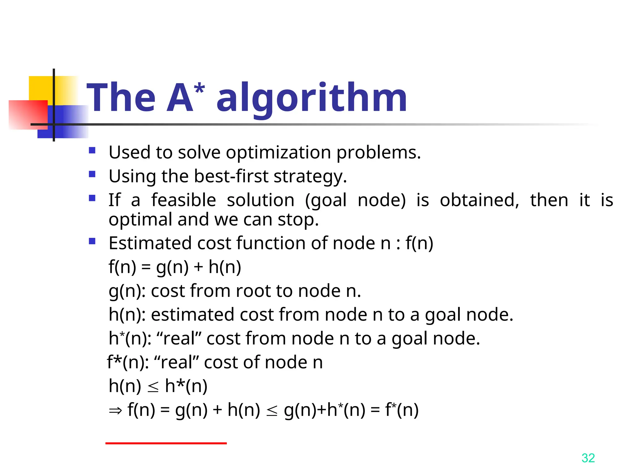
32.
32
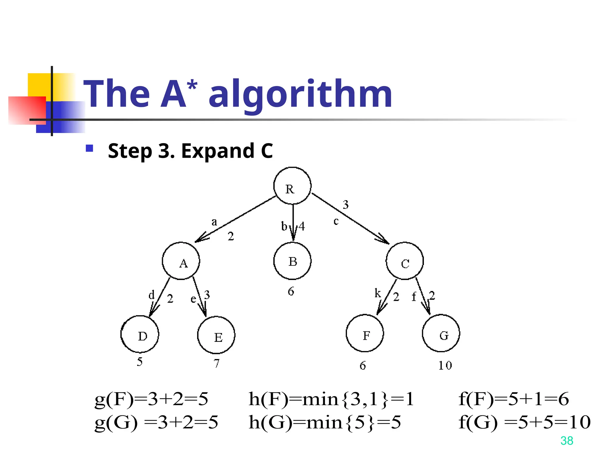
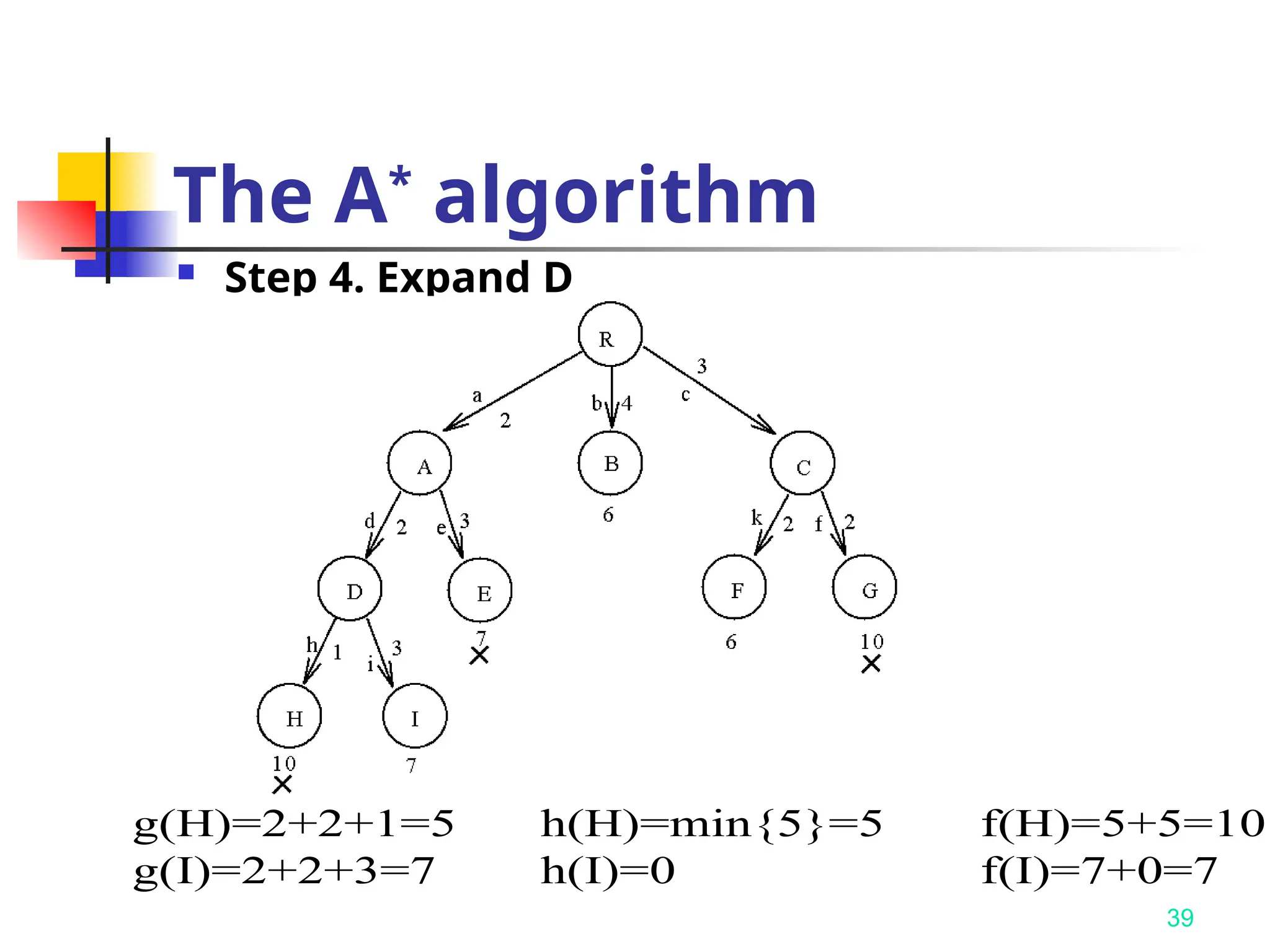
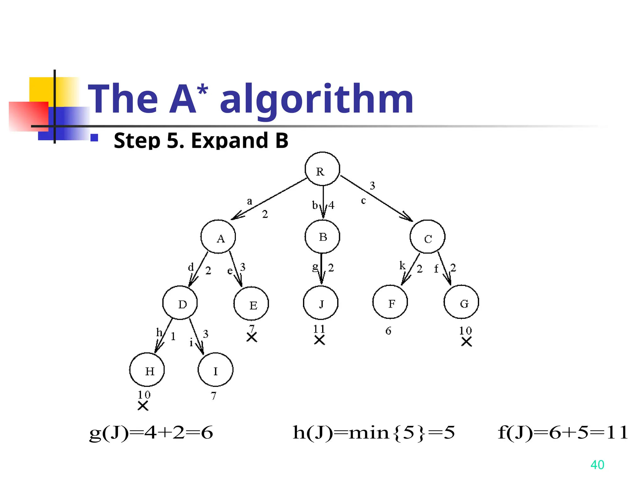
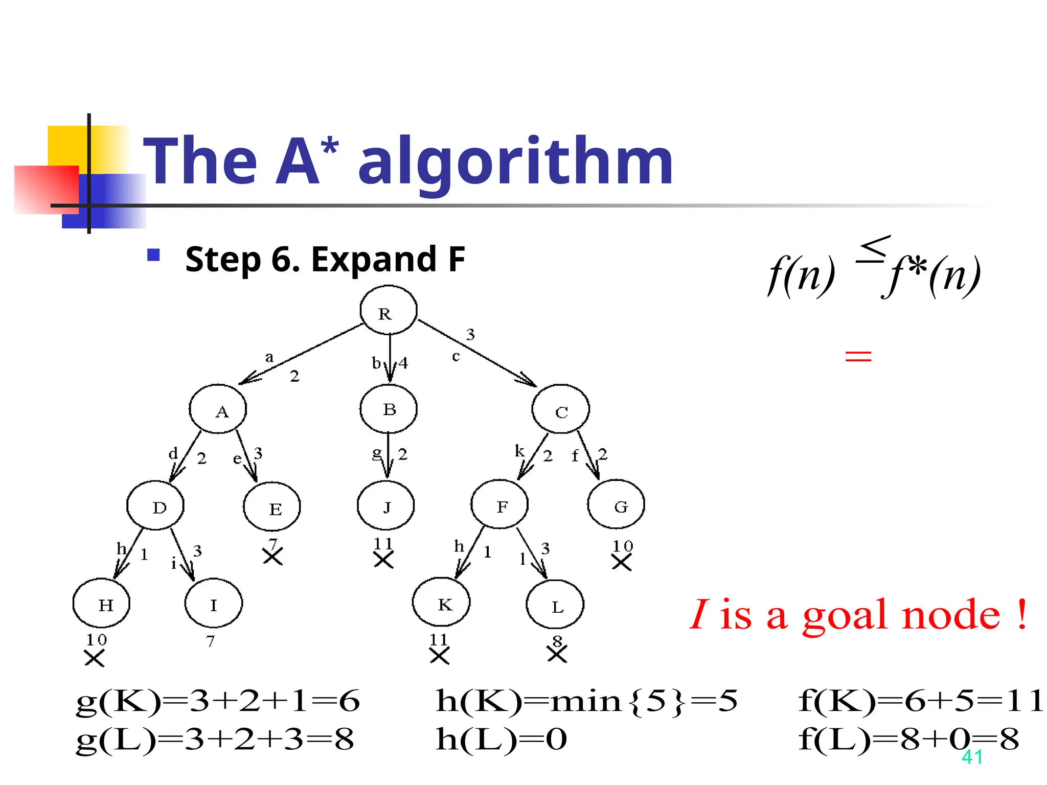
The A*
algorithm
Usedto solve optimization problems.
Using the best-first strategy.
If a feasible solution (goal node) is obtained, then it is
optimal and we can stop.
Estimated cost function of node n : f(n)
f(n) = g(n) + h(n)
g(n): cost from root to node n.
h(n): estimated cost from node n to a goal node.
h*
(n): “real” cost from node n to a goal node.
f*(n): “real” cost of node n
h(n) h*(n)
f(n) = g(n) + h(n) g(n)+h*
(n) = f*
(n)
33.
33
Reasoning
Let tbe the selected goal node. Let n de
note a node already expanded.
f(t)f(n)
f(t) f(n) f*(n)
But one of f*(n)’s must be the optimal va
lue (cost). Let f*(s) denote the value.
We have f(t) f*(s) …………(a)
34.
34
Reasoning
Since tis a goal node, we have h(t)=0.
Thus, f(t)=g(t)+h(t)=g(t).
By Eq. (a), we have f(t)=g(t)f*(s)
Yet, f(t)=g(t) is the value of a feasible so
lution. Consequently, g(t) cannot be sm
aller than f*(s) by definition. This means
that g(t)=f*(s).
35.
35
The A*
algorithm
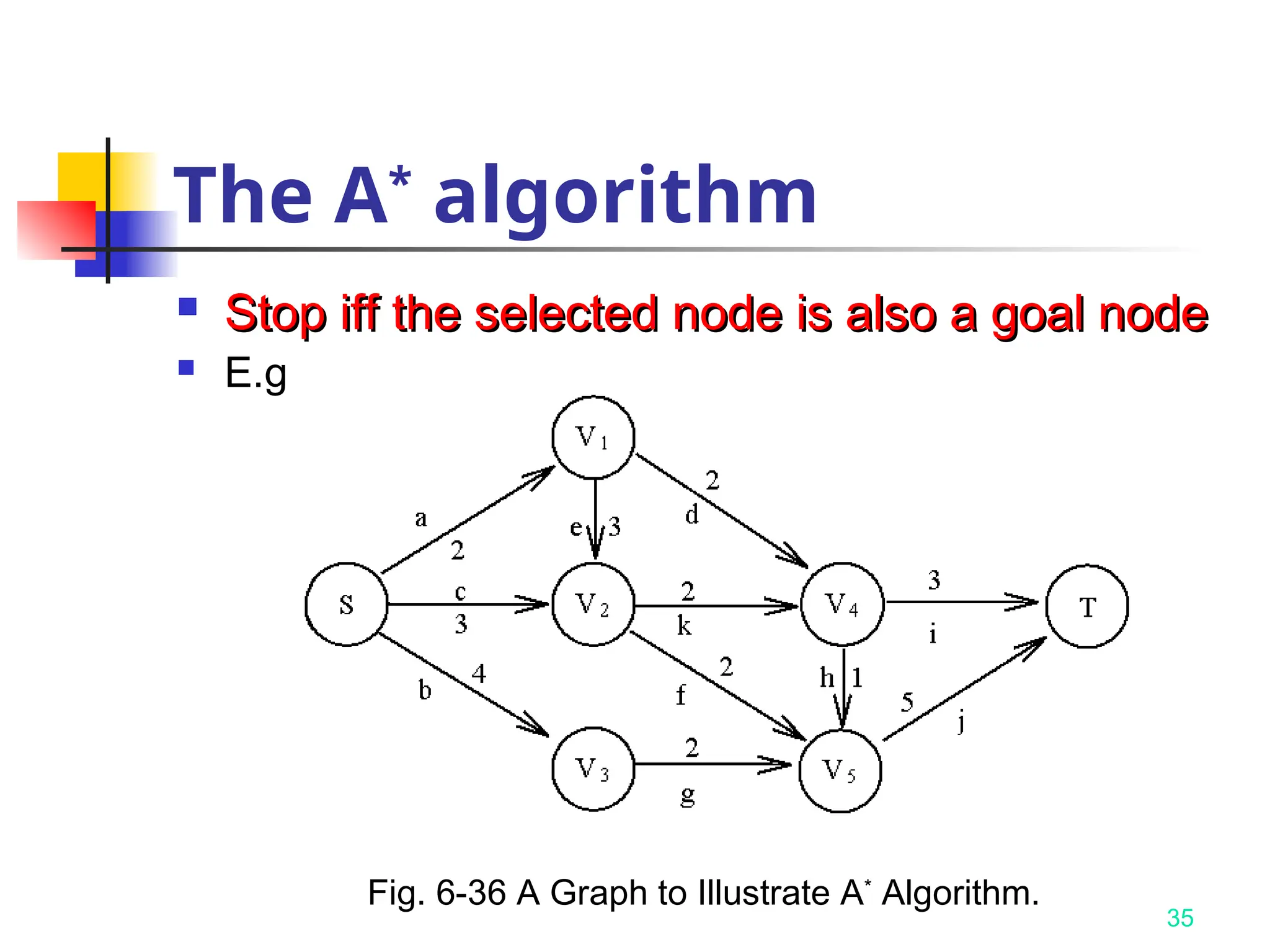
Stopiff the selected node is also a goal node
Stop iff the selected node is also a goal node
E.g.
Fig. 6-36 A Graph to Illustrate A*
Algorithm.