Downloaded 22 times
![
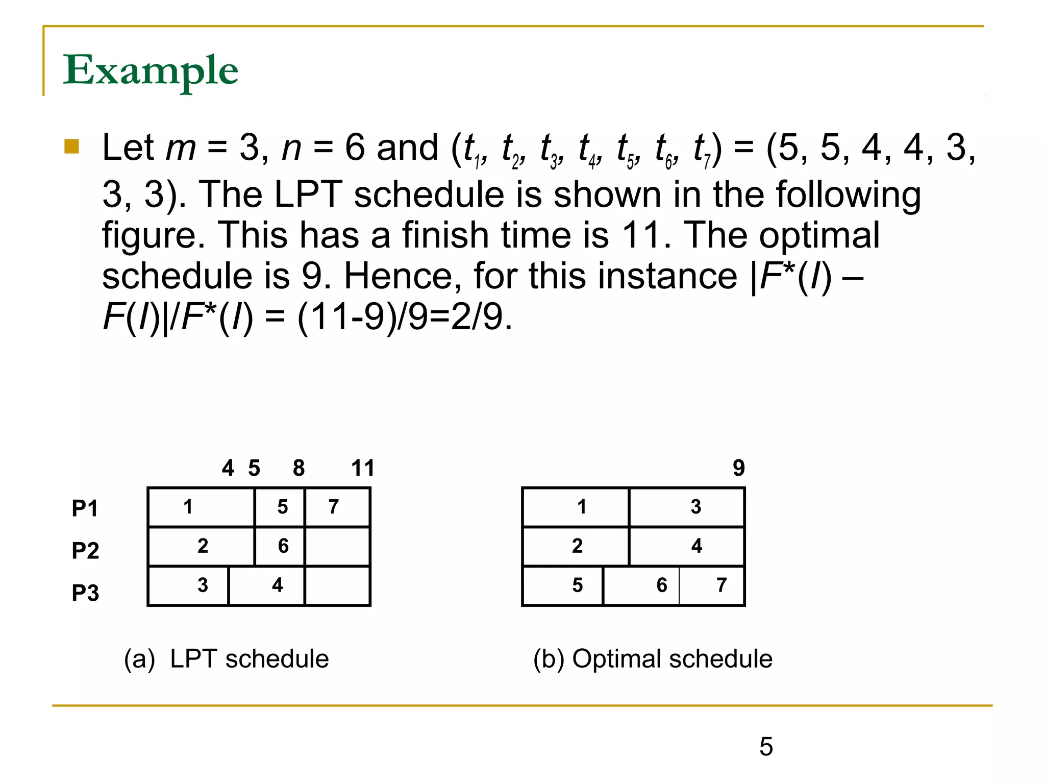
While the LPT rule may generate optimal schedules for
some problem instances, it does not do so for all
instances. How bad can LPT schedules be relative to
optimal schedules?
Theorem: [Graham] Let F*(I) be the finish time of an
optimal m processor schedule for instance I of the task
scheduling problem. Let F(I) be the finish time of an LPT
schedule for the same instance, then
|F*(I)-F(I)|/F*(I) ≤ 1/3 – 1/(3m)
The proof of this theorem can be referred to the book
“Fundamentals of Computer Algorithms”, E. Horowitz and
S. Sahni, Pitman Publishing, 1978.
6](https://image.slidesharecdn.com/chap8partii-140227195332-phpapp01/75/Chap8-part-ii-6-2048.jpg)


![
While the LPT rule may generate optimal schedules for
some problem instances, it does not do so for all
instances. How bad can LPT schedules be relative to
optimal schedules?
Theorem: [Graham] Let F*(I) be the finish time of an
optimal m processor schedule for instance I of the task
scheduling problem. Let F(I) be the finish time of an LPT
schedule for the same instance, then
|F*(I)-F(I)|/F*(I) ≤ 1/3 – 1/(3m)
The proof of this theorem can be referred to the book
“Fundamentals of Computer Algorithms”, E. Horowitz and
S. Sahni, Pitman Publishing, 1978.
6](https://crownmelresort.com/image.slidesharecdn.com/chap8partii-140227195332-phpapp01/75/Chap8-part-ii-6-2048.jpg)


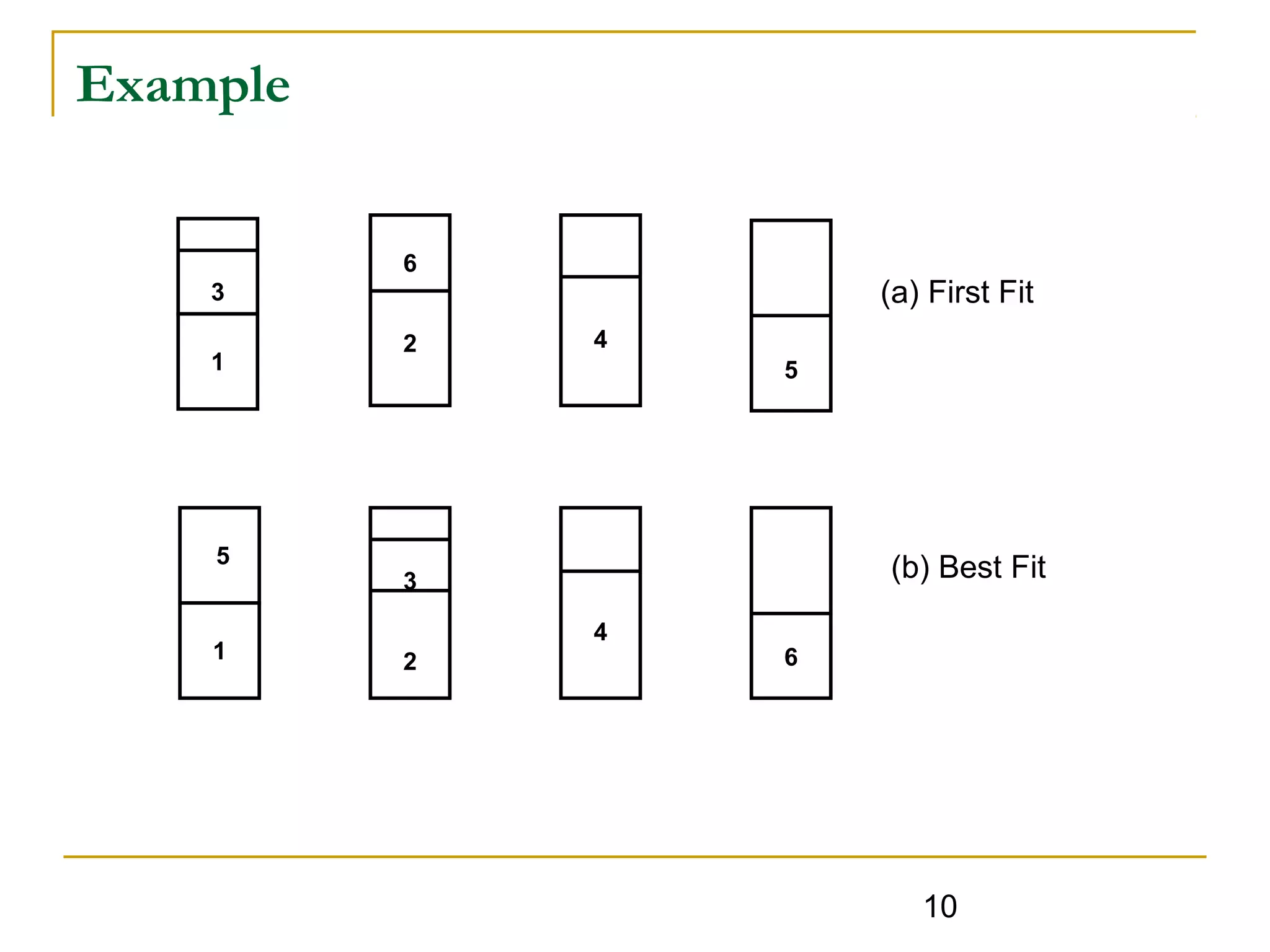
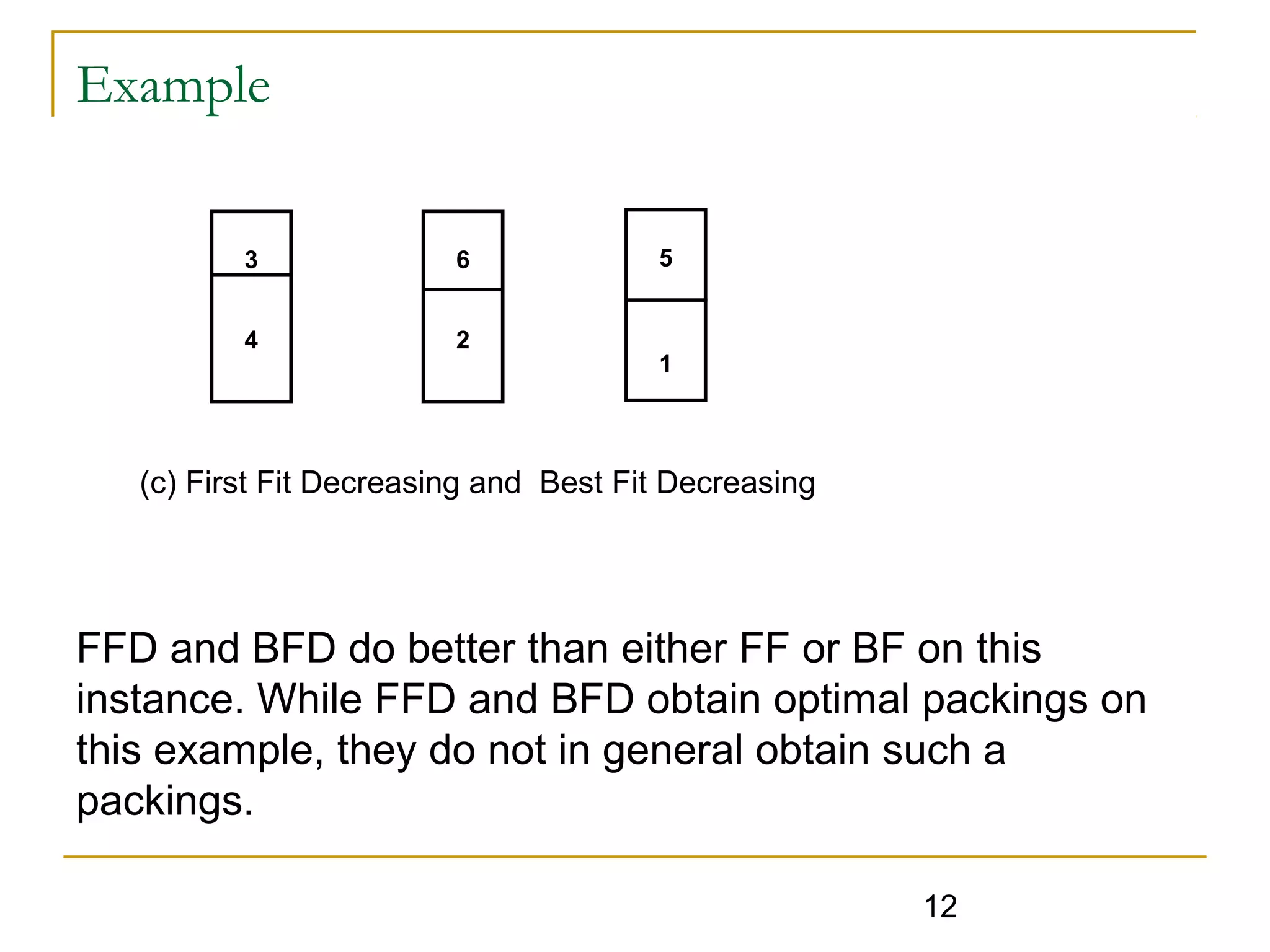
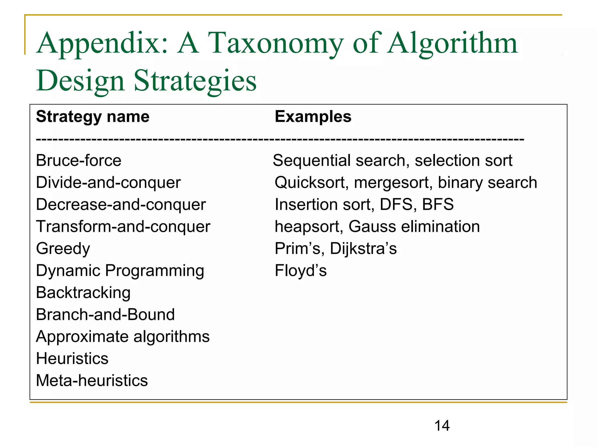
This document discusses approximation algorithms for two NP-complete problems: scheduling independent tasks and bin packing. It introduces the longest processing time (LPT) rule for scheduling tasks, and proves an upper bound on how suboptimal LPT schedules can be compared to optimal schedules. It also describes four heuristics for bin packing - first fit, best fit, first fit decreasing, and best fit decreasing - and proves an upper bound on the number of bins they may use compared to optimal packings.


![SHS_Core_CAE_Q3_LE1 FOR THIRD [FINAL].pdf](https://cdn.slidesharecdn.com/ss_thumbnails/shscorecaeq3le1final-251116055110-e3081055-thumbnail.jpg?width=640&height=640&fit=bounds)


