Downloaded 1,699 times

![Artificial Intelligence
• “ [The automation of] activities that we associate with
human thinking, activities such as decision-making,
problem solving, learning ..."(Bellman, 1978)
• "A field of study that seeks to explain and emulate
intelligent behavior in terms of computational processes"
(Schalkoff, 1 990)
• “The capability of a machine to immitate intellignet
human behavior”. (merriam-webster)
Footer Text 3](https://image.slidesharecdn.com/aimldlgenesys-160818184429/75/Artificial-Intelligence-Machine-Learning-and-Deep-Learning-3-2048.jpg)

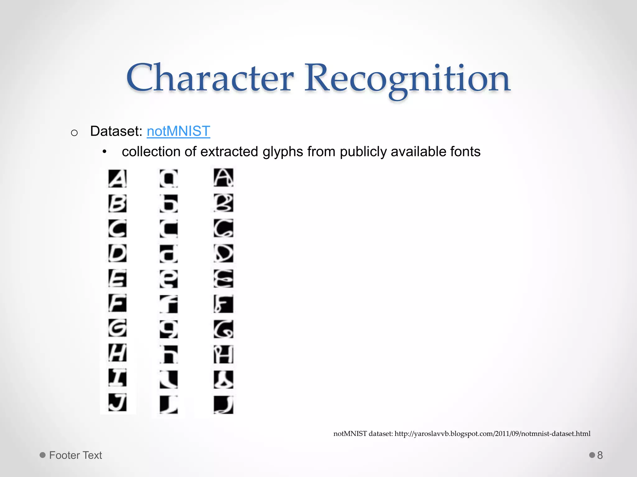
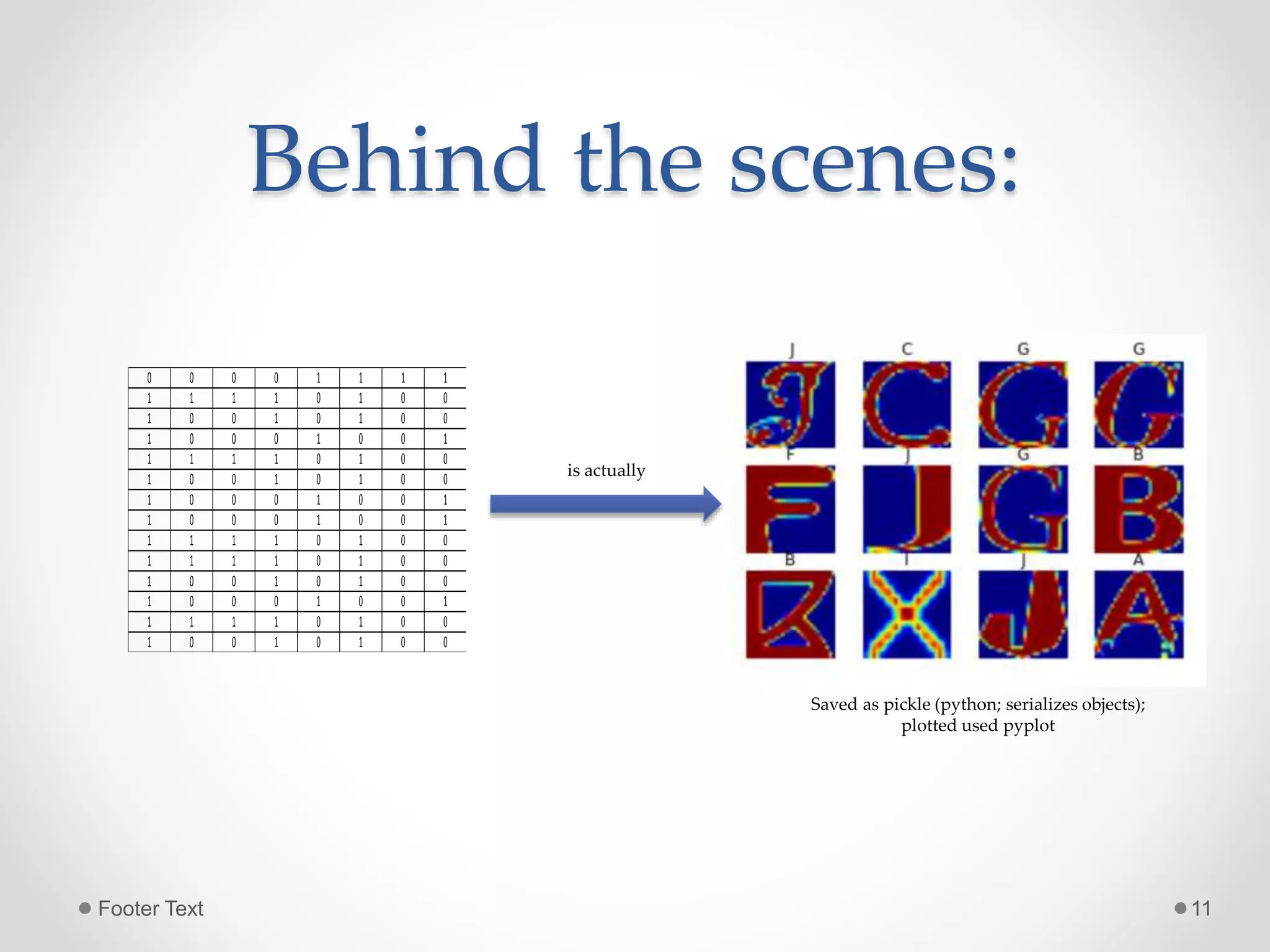
![Character Recognition
function = LogisticRegression()
features_testset =
test_dataset.reshape(test_dataset.shape[0], 28 * 28)
labels_testset = test_labels
feature_trainingset =
train_dataset[:sample_size].reshape(sample_size,
28*28)
labels_traininigset = train_labels[:sample_size]
function.fit(feature_trainingset, labels_traininigset)
function.score(features_testset, labels_testset)
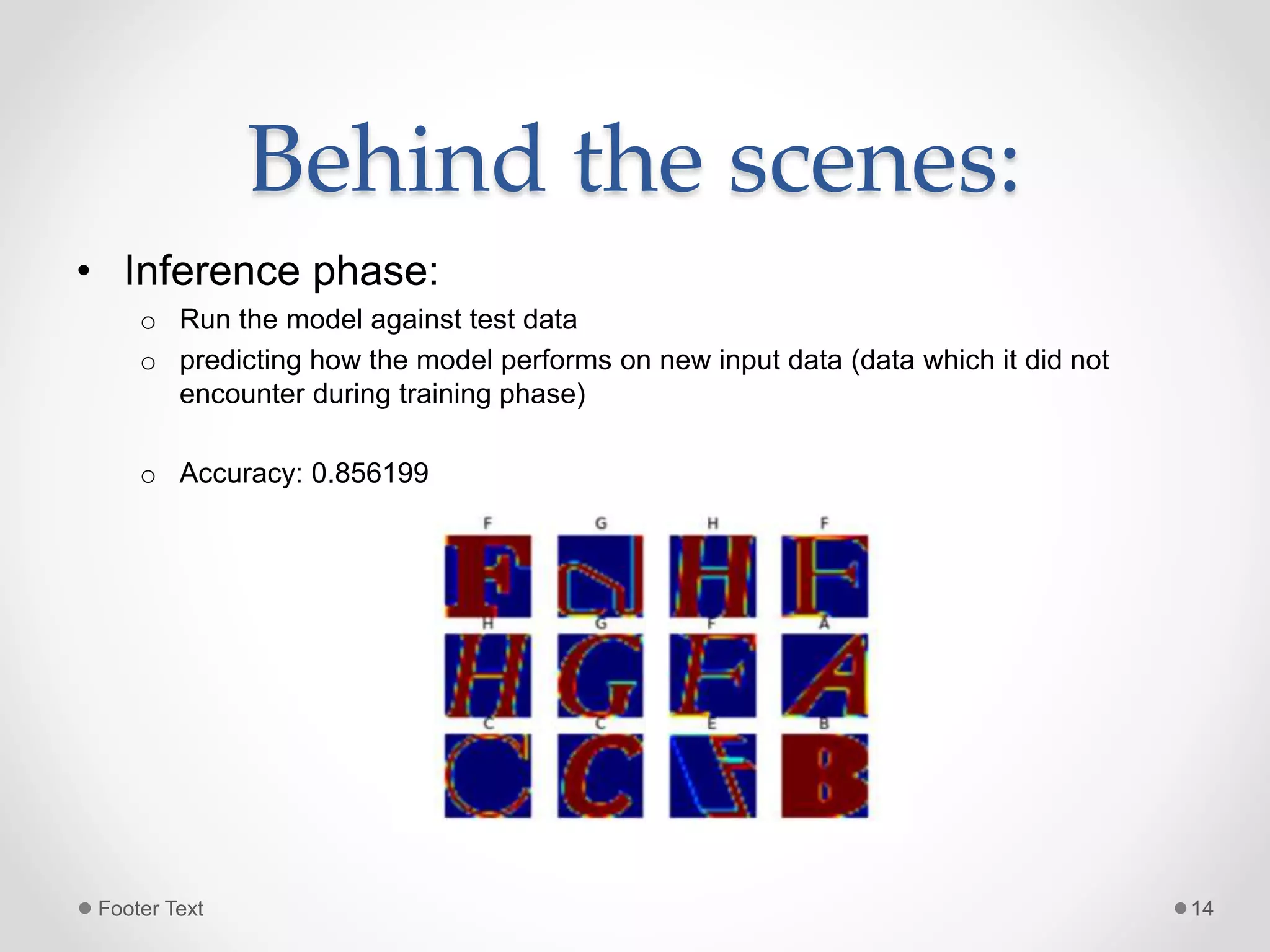
Accuracy: 0.856199
prepare
model;
learn weights
prediction/
inference
evaluation
*Library: Scikit-learn
Footer Text 9](https://image.slidesharecdn.com/aimldlgenesys-160818184429/75/Artificial-Intelligence-Machine-Learning-and-Deep-Learning-9-2048.jpg)


![Artificial Intelligence
• “ [The automation of] activities that we associate with
human thinking, activities such as decision-making,
problem solving, learning ..."(Bellman, 1978)
• "A field of study that seeks to explain and emulate
intelligent behavior in terms of computational processes"
(Schalkoff, 1 990)
• “The capability of a machine to immitate intellignet
human behavior”. (merriam-webster)
Footer Text 3](https://crownmelresort.com/image.slidesharecdn.com/aimldlgenesys-160818184429/75/Artificial-Intelligence-Machine-Learning-and-Deep-Learning-3-2048.jpg)


![Character Recognition
function = LogisticRegression()
features_testset =
test_dataset.reshape(test_dataset.shape[0], 28 * 28)
labels_testset = test_labels
feature_trainingset =
train_dataset[:sample_size].reshape(sample_size,
28*28)
labels_traininigset = train_labels[:sample_size]
function.fit(feature_trainingset, labels_traininigset)
function.score(features_testset, labels_testset)
Accuracy: 0.856199
prepare
model;
learn weights
prediction/
inference
evaluation
*Library: Scikit-learn
Footer Text 9](https://crownmelresort.com/image.slidesharecdn.com/aimldlgenesys-160818184429/75/Artificial-Intelligence-Machine-Learning-and-Deep-Learning-9-2048.jpg)


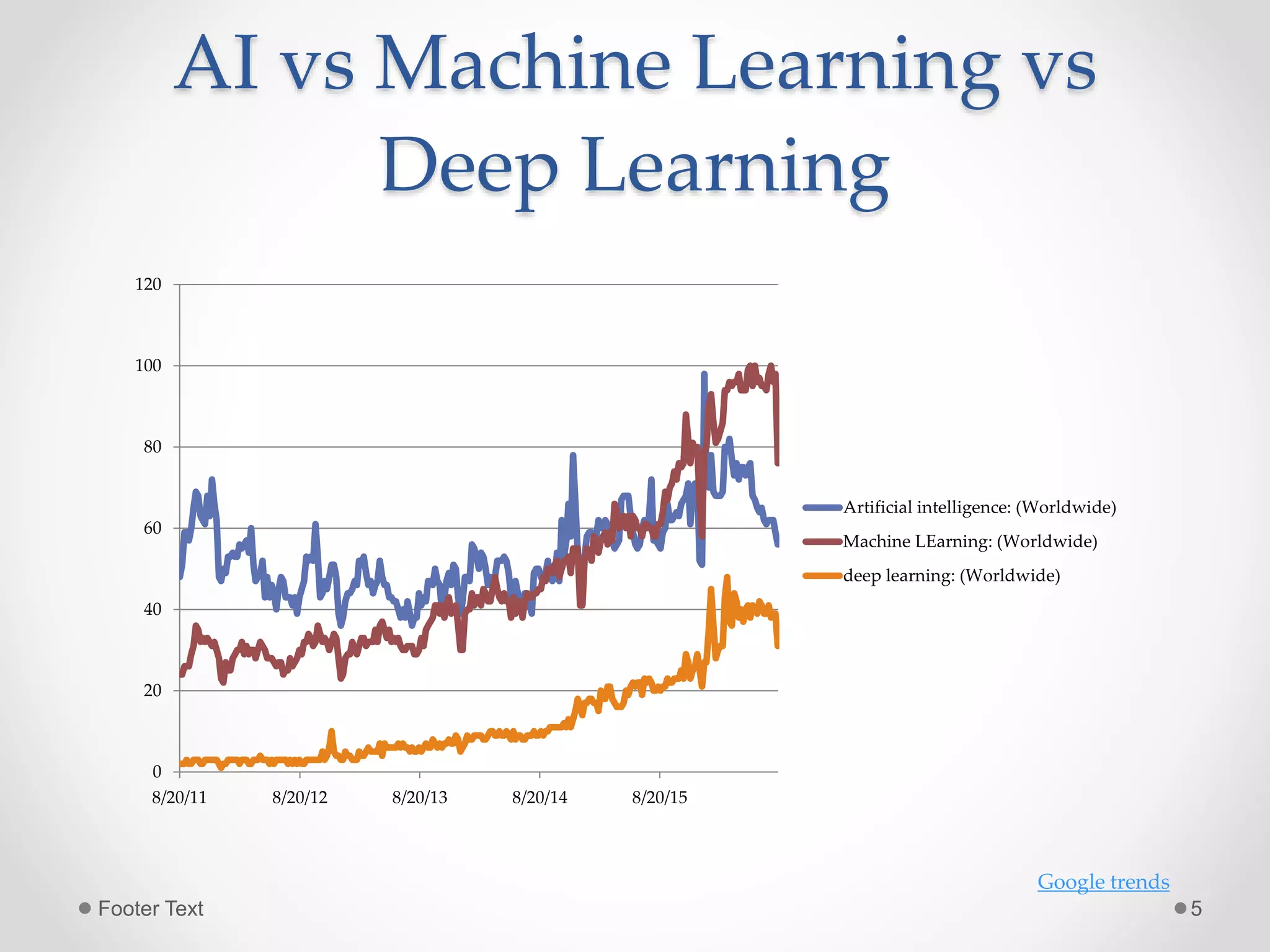
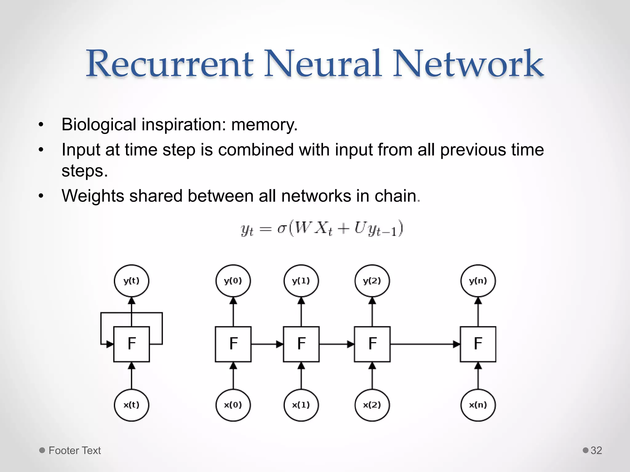
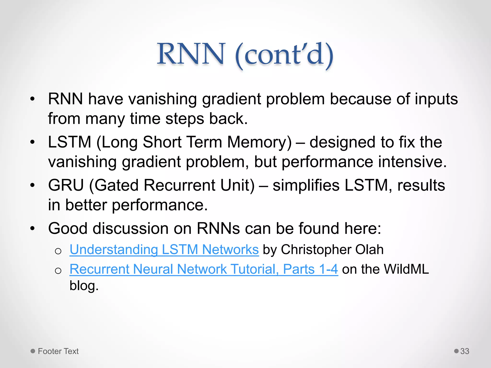
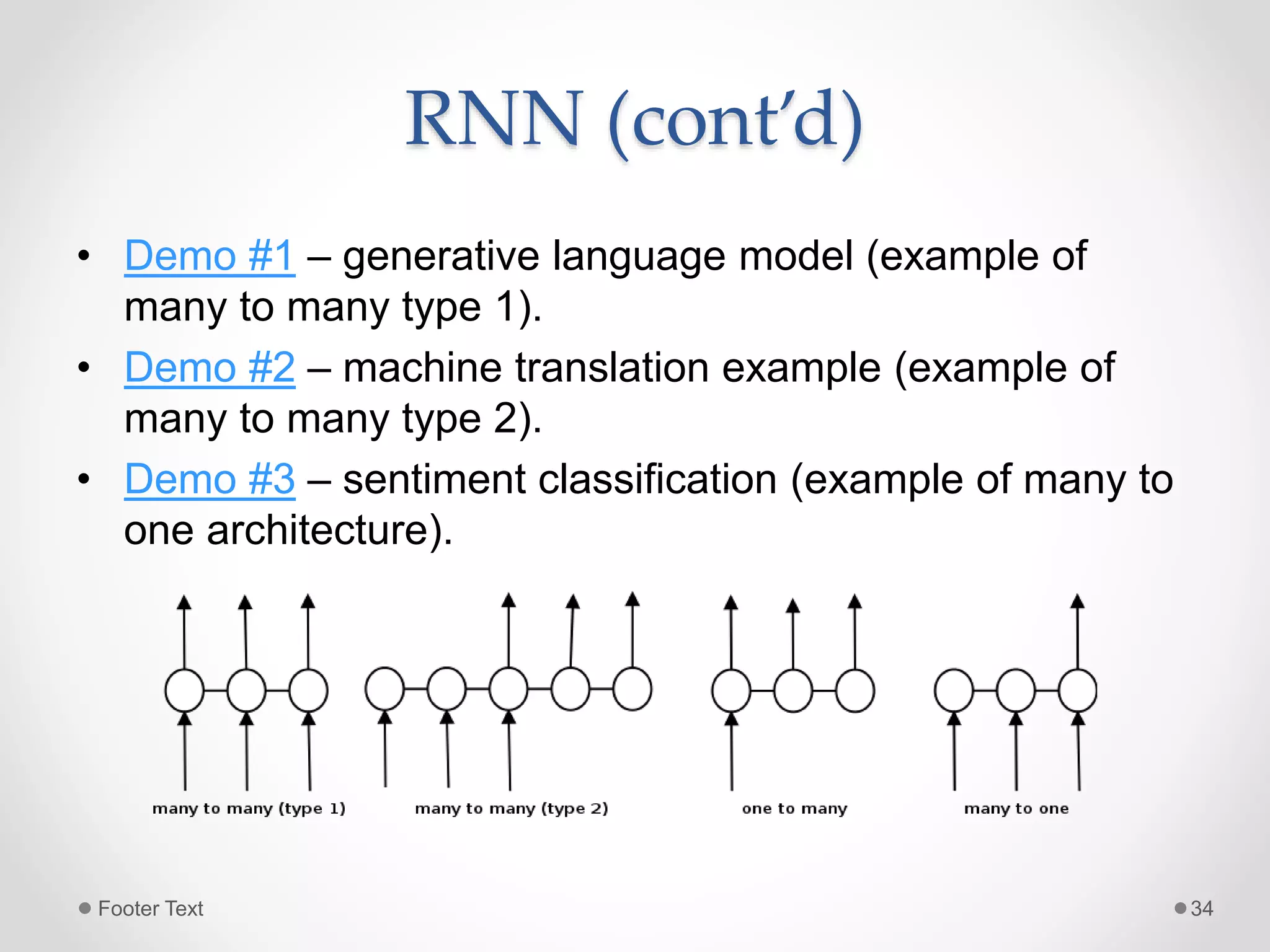
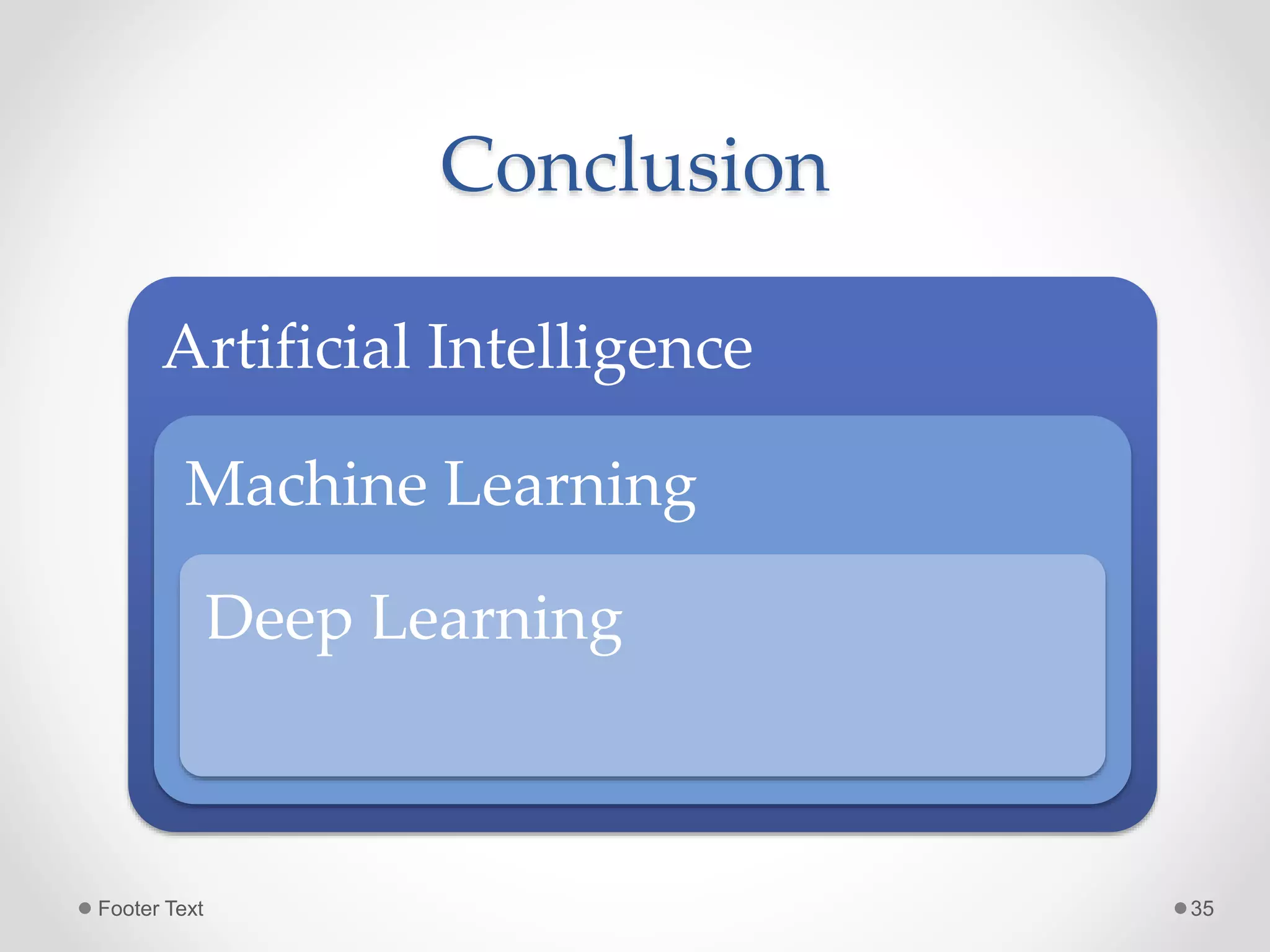
The document provides an overview of artificial intelligence, machine learning, and deep learning, highlighting their definitions, examples, and distinctions. It covers machine learning approaches, including algorithms, feature extraction, and gradient descent methods, as well as deep learning architectures like fully connected networks, convolutional neural networks, and recurrent neural networks. Additionally, it discusses the importance of data, the need for deep learning, and offers resources for further learning.