Agricultural statistics - Statistical science JRF / ICAR AIEEA note by Subham Mandal
Statistics
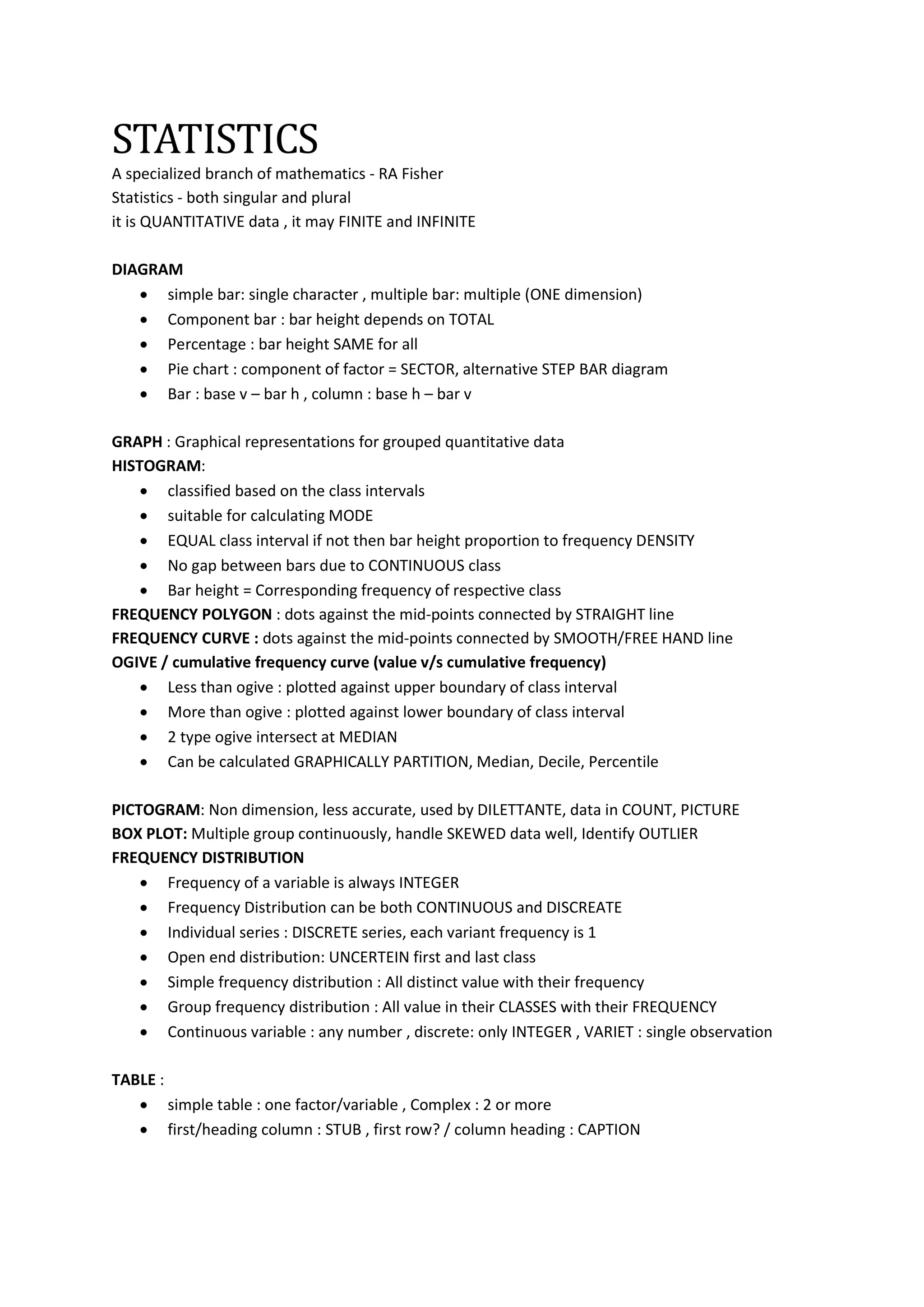
Diagram
Graph
Histogram
Frequency Polygon
Ogive
Pictogram
Box Plot
Frequency Distribution
Central Tendency
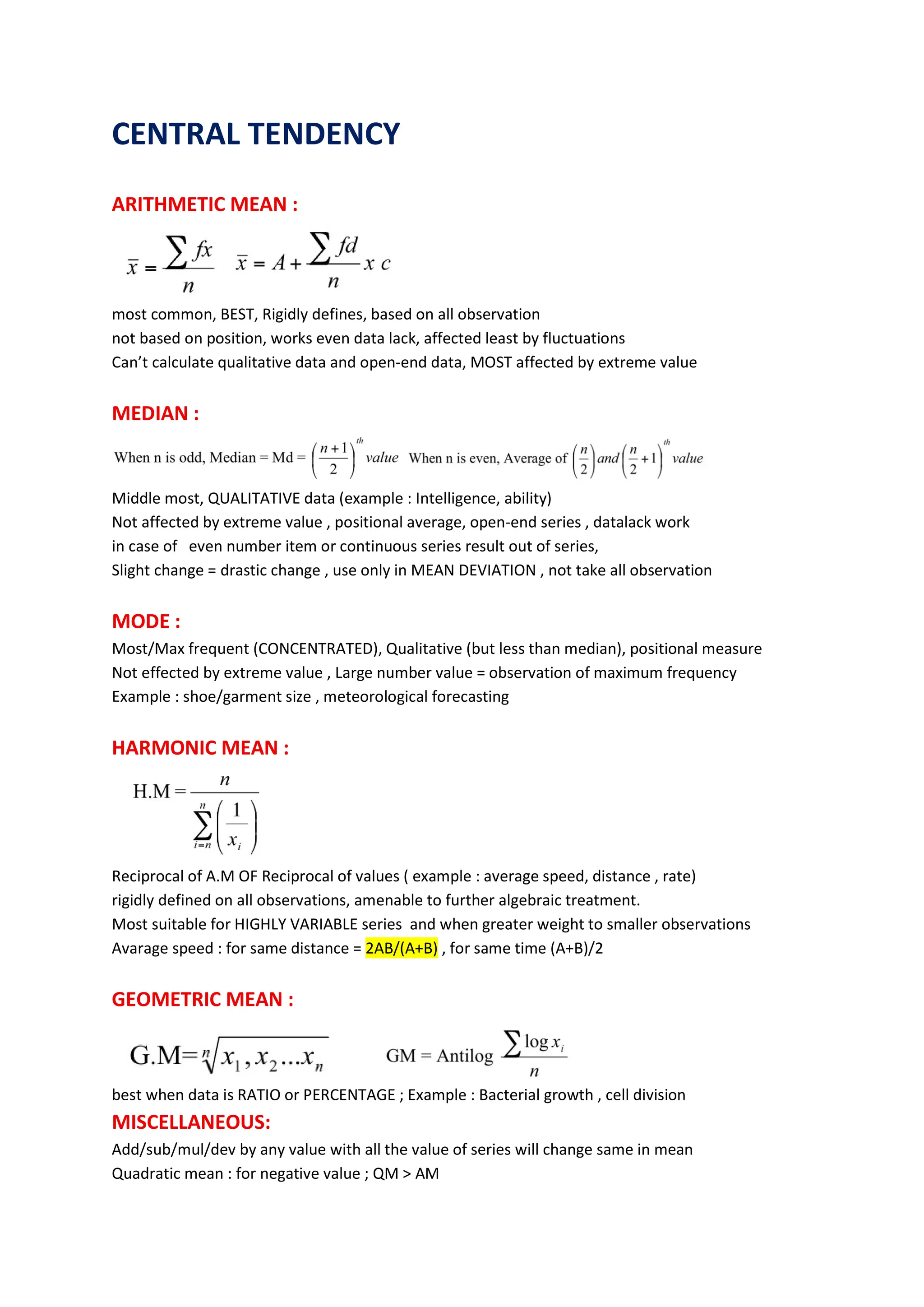
Arithmetic Mean
Median
Mode
Harmonic Mean
Geometric Mean
Am >= Gm >= Hm
Symmetrical Distribution
Skewed Distribution
Dispersion
Range
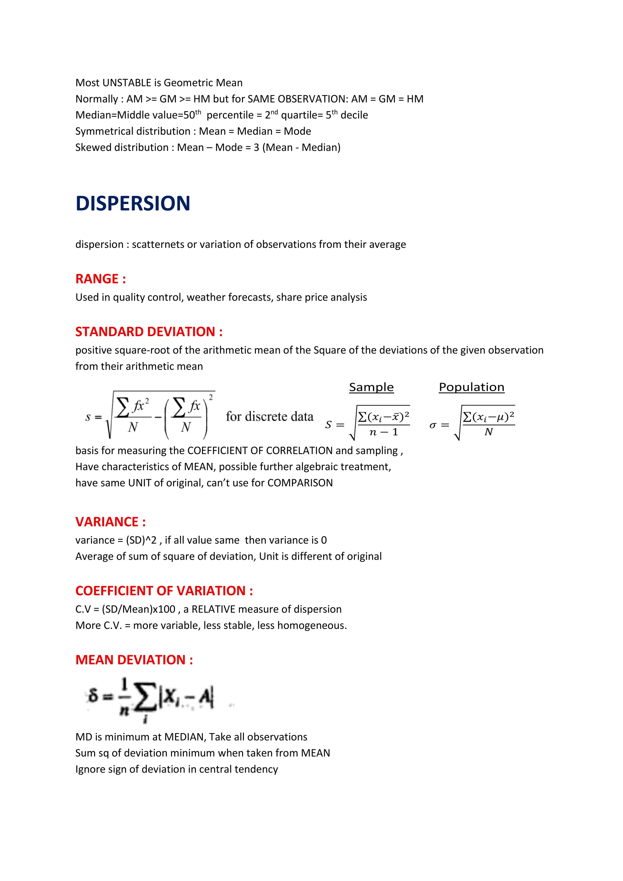
Standard Deviation
Variance
Coefficient Of Variation
Mean Deviation
Quartile Deviation
Skewness
Kerl Perason’s Skewness
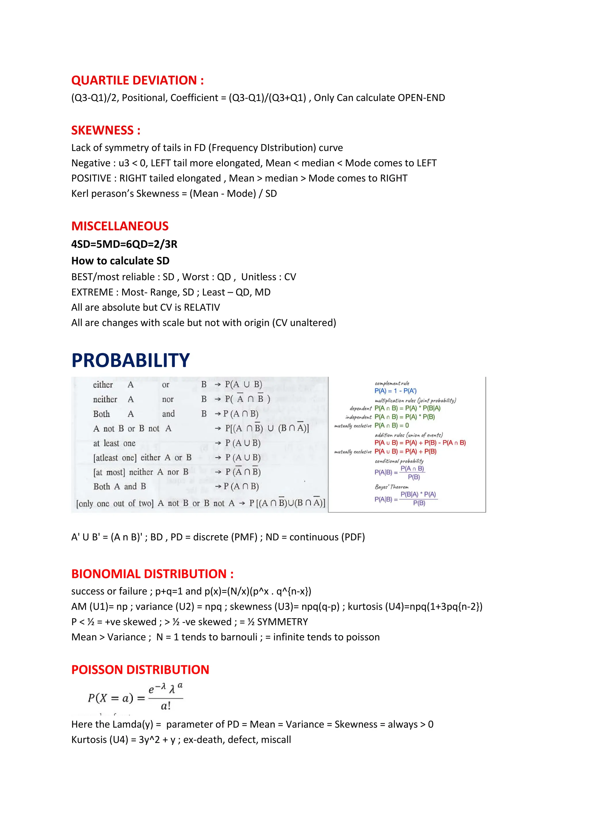
Probability
Bionomial
Poisson Distribution
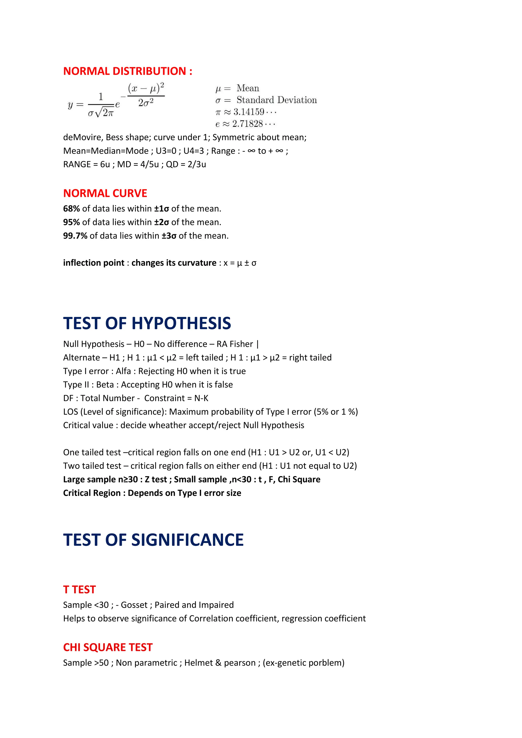
Normal Distribution
Normal Curve
Inflection Point
Test Of Hypothesis
Null Hypothesis
Alternate Hypothesis
Type I Type Ii Error
Level Of Significance
Critical Value One Tailed Test Two Tailed
Test Of Significance
T Test
Chi Square Test
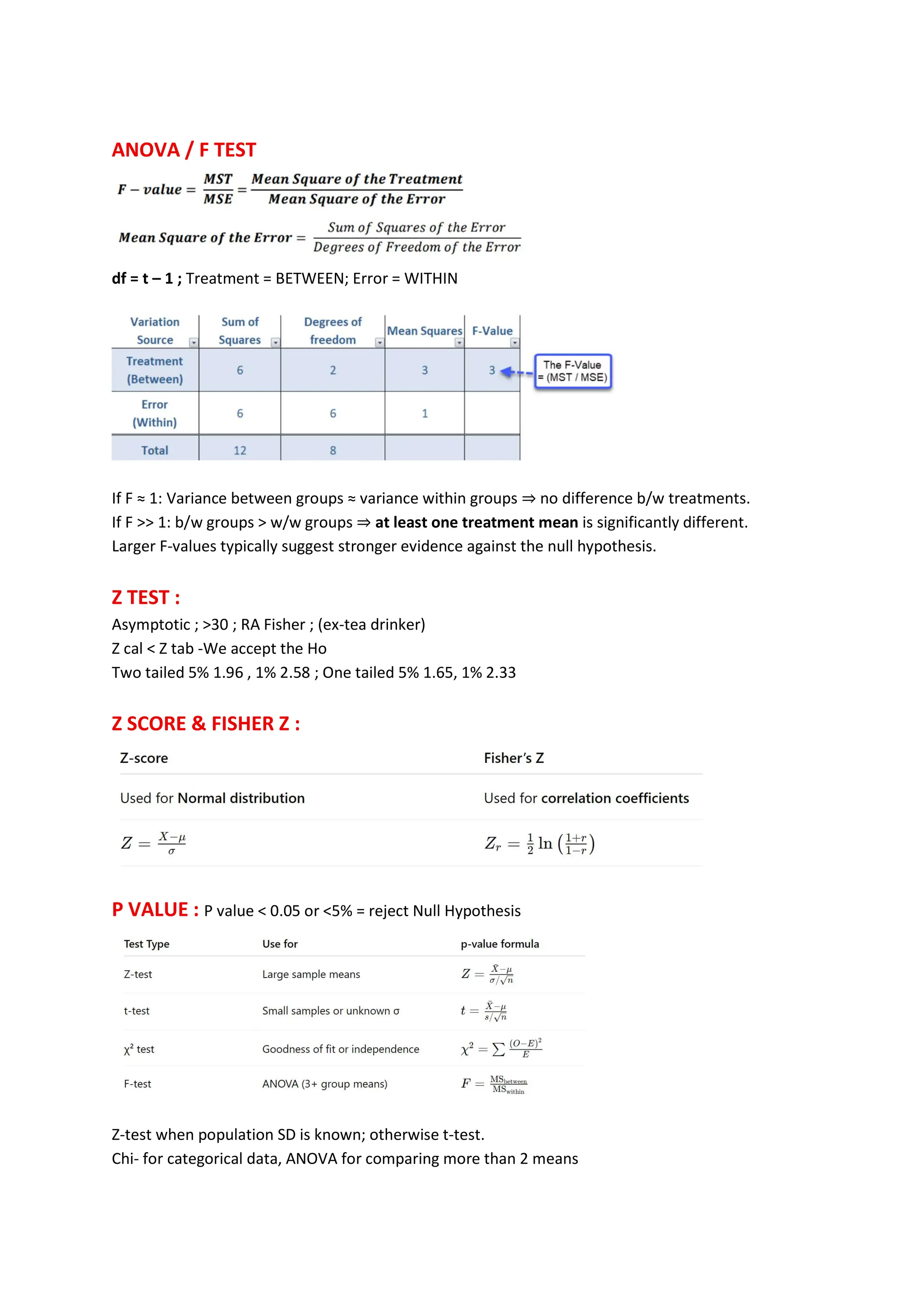
Anova / F Test
Z Test
Z Score & Fisher Z :
P Value
Error
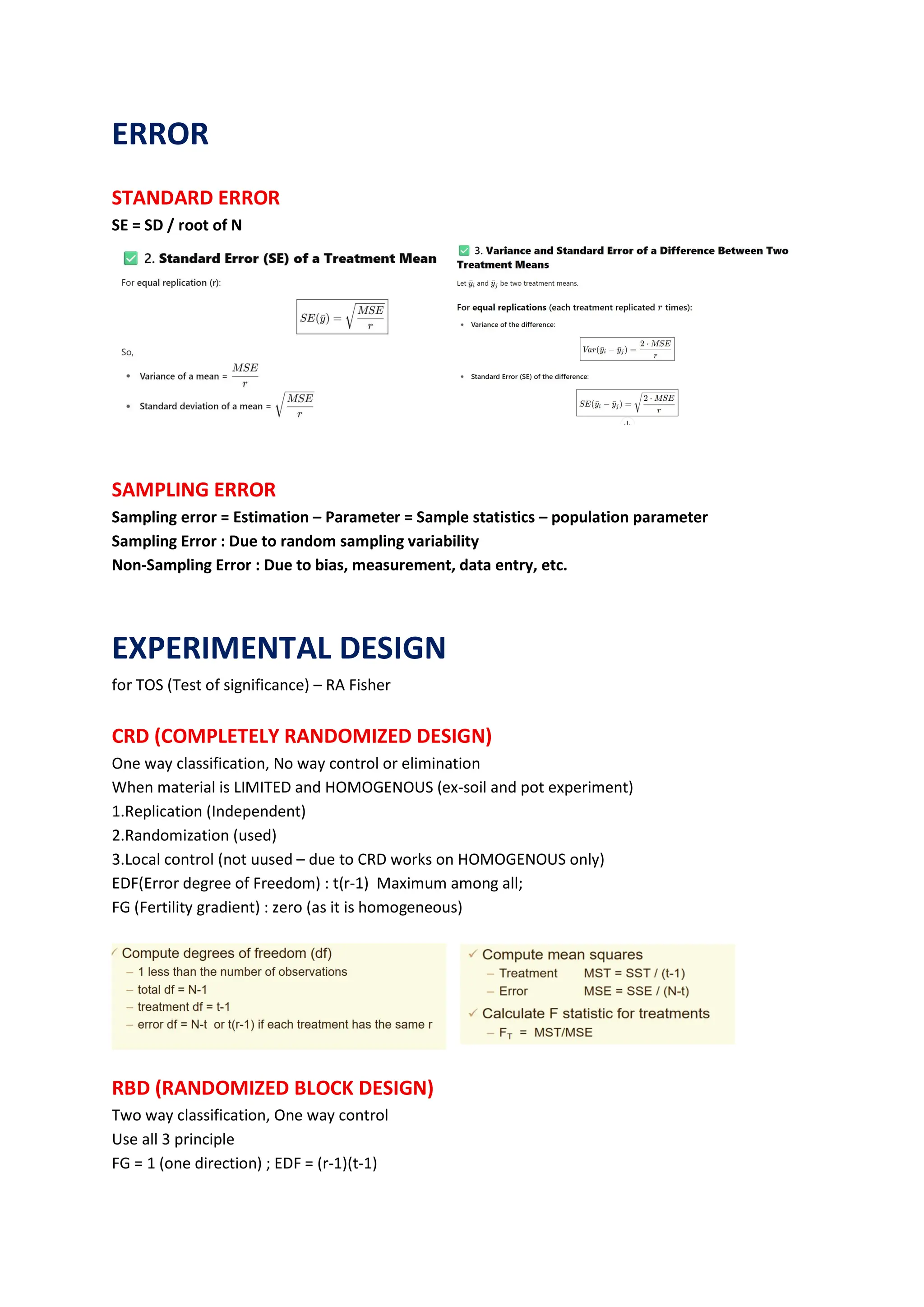
Standard Error
Sampling Error
Experimental Design
Crd (Completely Randomized Design)
Edf(Error Degree Of Freedom)
Rbd (Randomized Block Design)
Lsd (Latent Square Design) :
Spd (Split Plot Design)
Correlation Regression :
Correlation :
Regression :
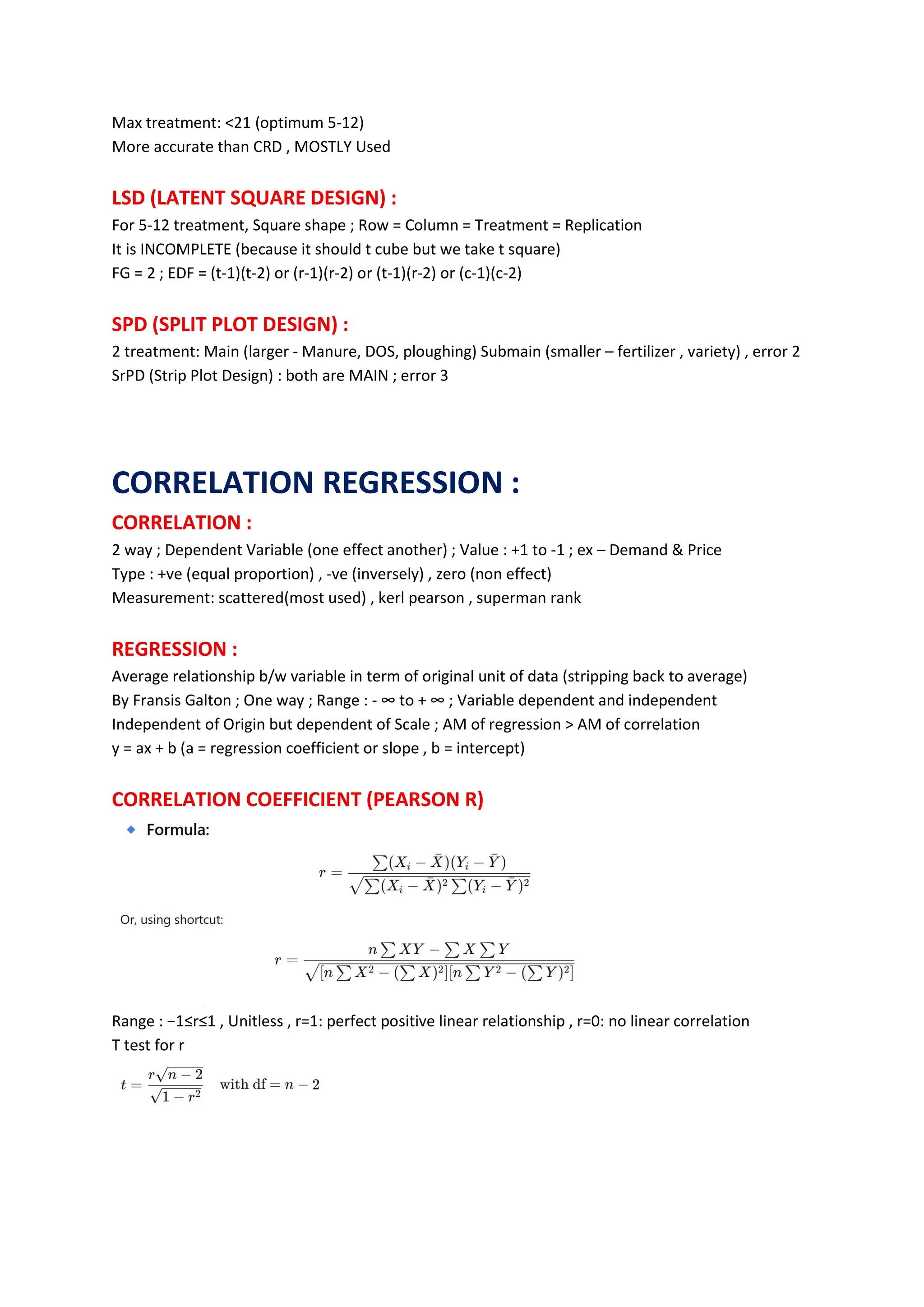
Correlation Coefficient (Pearson R)
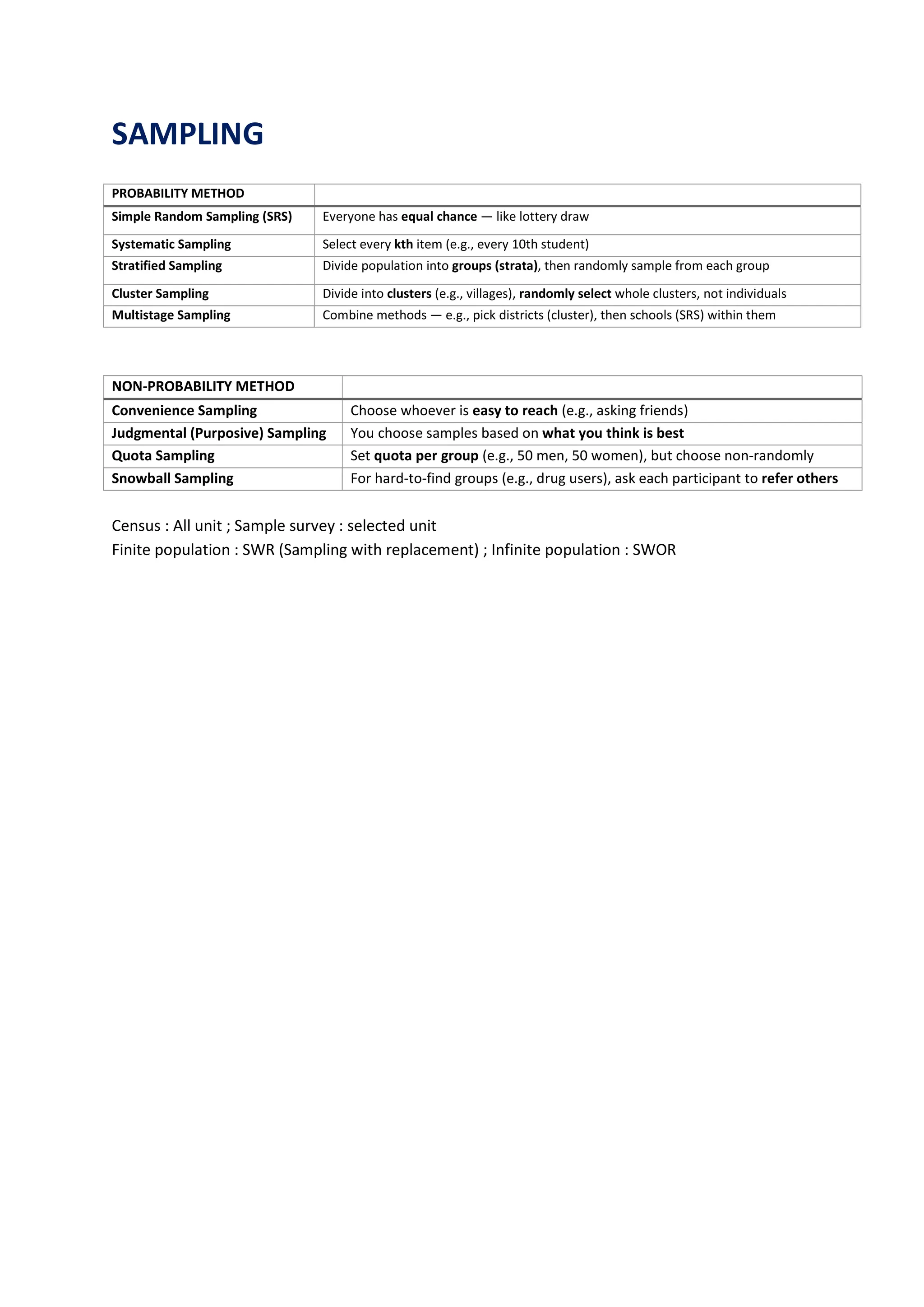
Probability Method
Non-Probability Method


![SHS_Core_CAE_Q3_LE1 FOR THIRD [FINAL].pdf](https://cdn.slidesharecdn.com/ss_thumbnails/shscorecaeq3le1final-251116055110-e3081055-thumbnail.jpg?width=640&height=640&fit=bounds)


