This paper aims to explore models based on the extreme gradient boosting (XGBoost) approach for business risk classification. Feature selection (FS) algorithms and hyper-parameter optimizations are simultaneously considered during model training. The five most commonly used FS methods including weight by Gini, weight by Chi-square, hierarchical variable clustering, weight by correlation, and weight by information are applied to alleviate the effect of redundant features. Two hyper-parameter optimization approaches, random search (RS) and Bayesian tree-structuredParzen Estimator (TPE), are applied in XGBoost. The effect of different FS and hyper-parameter optimization methods on the model performance are investigated by the Wilcoxon Signed Rank Test. The performance of XGBoost is compared to the traditionally utilized logistic regression (LR) model in terms of classification accuracy, area under the curve (AUC), recall, and F1 score obtained from the 10-fold cross validation. Results show that hierarchical clustering is the optimal FS method for LR while weight by Chi-square achieves the best performance in XG-Boost. Both TPE and RS optimization in XGBoost outperform LR significantly. TPE optimization shows a superiority over RS since it results in a significantly higher accuracy and a marginally higher AUC, recall and F1 score. Furthermore, XGBoost with TPE tuning shows a lower variability than the RS method. Finally, the ranking of feature importance based on XGBoost enhances the model interpretation. Therefore, XGBoost with Bayesian TPE hyper-parameter optimization serves as an operative while powerful approach for business risk modeling
![International Journal of Database Management Systems (IJDMS ) Vol.11, No.1, February 2019
DOI : 10.5121/ijdms.2019.11101 1
A XGBOOST RISK MODEL VIA FEATURE
SELECTION AND BAYESIAN HYPER-PARAMETER
OPTIMIZATION
Yan Wang1
and Xuelei Sherry Ni2
1
Graduate College, Kennesaw State University, Kennesaw, USA
2
Department of Statistics and Analytical Sciences, Kennesaw State University,
Kennesaw, USA
ABSTRACT
This paper aims to explore models based on the extreme gradient boosting (XGBoost) approach for
business risk classification. Feature selection (FS) algorithms and hyper-parameter optimizations are
simultaneously considered during model training. The five most commonly used FS methods including
weight by Gini, weight by Chi-square, hierarchical variable clustering, weight by correlation, and weight
by information are applied to alleviate the effect of redundant features. Two hyper-parameter optimization
approaches, random search (RS) and Bayesian tree-structuredParzen Estimator (TPE), are applied in
XGBoost. The effect of different FS and hyper-parameter optimization methods on the model performance
are investigated by the Wilcoxon Signed Rank Test. The performance of XGBoost is compared to the
traditionally utilized logistic regression (LR) model in terms of classification accuracy, area under the
curve (AUC), recall, and F1 score obtained from the 10-fold cross validation. Results show that
hierarchical clustering is the optimal FS method for LR while weight by Chi-square achieves the best
performance in XG-Boost. Both TPE and RS optimization in XGBoost outperform LR significantly. TPE
optimization shows a superiority over RS since it results in a significantly higher accuracy and a
marginally higher AUC, recall and F1 score. Furthermore, XGBoost with TPE tuning shows a lower
variability than the RS method. Finally, the ranking of feature importance based on XGBoost enhances the
model interpretation. Therefore, XGBoost with Bayesian TPE hyper-parameter optimization serves as an
operative while powerful approach for business risk modeling.
KEYWORDS
Extreme gradient boosting; XGBoost; feature selection; Bayesian tree-structured Parzen estimator; risk
modeling
1. INTRODUCTION
Risk modeling is an effective tool to assist financial institutions to properly decide
whether or not to grant loans to business or other applicants [1]. Thereby, the problem of
risk modeling is transformed into a binary classification task, i.e., grant loans to low risk
applicants or not grant to those with high risk. Logistic regression (LR) is a traditionally
utilized technique for binary classificationsin the financial domain because of its easy
implementation, explainable results, as well as the similar and often better performance
compared to other binary classifiers such as decision trees and neural networks [2] [3]
[4] [5] [6]. On the other hand, it has been shown that a single classifier cannot solve all
problems effectively while ensemble models have been revealed to be promising in
many credit risk studies [7] [8] [9]. One of the state-of-the-art ensemble approach is the
extreme gradient boosting (XGBoost). It is a novel while advanced variant of the](https://image.slidesharecdn.com/11119ijdms01-250312052208-d221ec1a/75/A-Xgboost-Risk-Model-Via-Feature-Selection-and-Bayesian-Hyper-Parameter-Optimization-1-2048.jpg)
![International Journal of Database Management Systems (IJDMS ) Vol.11, No.1, February 2019
2
gradient boosting algorithm and has obtained promising results in many Kaggle machine
learning competitions [10]. Furthermore, XGBoost has been successfully applied in
bankruptcy prediction and credit scoringin a few studies[11][12].
Numerous studies have focused on offering novel mechanisms to enhance the
performance of credit risk modeling. It has been demonstrated that feature selection (FS)
is one of the efficient approaches in improving model performance because of its ability
to alleviate the effects of noise and redundant variables [13]. Another method for model-
improving is the hyper-parameter optimization or tuning. It is shown that careful hyper-
parameter tuning tends to prevent the failure and reduce the over-fitting problem of
XGBoost. The two main strategies used for finding the proper setting of hyper-
parameters in XGBoost are random search (RS) and Bayesian tree-structured Parzen
estimator (TPE). They have demonstrated substantial influence on classification
performance [14] [15].
After careful paper review, we find that there is seldom research aiming at exploring the
effect of FS and hyper-parameter optimizations simultaneously on XGBoost in the
financial domain. Therefore, motivated by the aforementioned studies, we set up a series
of experiments that contain FS methods and hyper-parameter optimizations
simultaneously, thereby exploring an accurate and comprehensive business risk model
based on XGBoost. The superiority of XGBoost over the widely used LR is evaluated
via classification accuracy, area under the curve (AUC), recall, and F1 score. Moreover,
the effect of different FS as well as hyper-parameter optimization methods on the model
performance is comprehensively investigated through the Wilcoxon signed rank test.
Finally, the features are ranked according to their importance score to enhance the model
interpretation.
This paper has been structured as follows. Since different FS methods and XGBoost
models along with the hyper-parameter optimization are used in this study, we will first
describe the relevant algorithms in Section 2. Then the experimental design is discussed
in Section 3. Section 4 demonstrates the experimental results and discussions.Finally,
Section 5 addresses the conclusions.
2. ALGORITHMS
In this section, the algorithms related to FS and XGBoost along with hyper-parameter
optimizations are discussed.
2.1. FEATURE SELECTION METHODS
FS methods aims to filter the redundant variables and select the most appropriate subset of
features. By applying FS methods to the dataset, we can decrease the effect of the noise as
well as reduce the computational cost during the modeling stage. Many studies have shown
that FS can be used to increase the classification performance [13] [16].
In this study, five commonly used FS methods are applied and evaluated: weight by gini
index, weight by chi-square, hierarchical variable clustering, weight by correlation, and
weight by information gain ratio. For simplicity, we use the terms with initial capitalization
to denote different FS methods. Therefore, Gini, Chi-square, Cluster, Correlation, and
Information are used to represent the aforementioned five FS approaches, respectively. In the
Gini FS method, the value of an attribute is evaluated via the gini impurity index. Similarly,
Chi-square, Correlation, and Information evaluates the relevance of the feature by calculating
its chi-squared statistic, correlation, and information gain ratio with respect to the target
variable [17]. Features with higher values of gini index, chi-squared statistic, correlation, and](https://image.slidesharecdn.com/11119ijdms01-250312052208-d221ec1a/75/A-Xgboost-Risk-Model-Via-Feature-Selection-and-Bayesian-Hyper-Parameter-Optimization-2-2048.jpg)
![International Journal of Database Management Systems (IJDMS ) Vol.11, No.1, February 2019
3
information gain ratio are selected in the FS results. On the other hand, the Cluster method
bases on the variable clustering analysis and selects the best feature within each cluster
according to the 1-R2
ratio defined in Eq. 1 [18]. Different from the rest of the four FS
methods, features with lower 1-R2
ratio are selected by the Cluster method.
1 − =
1 − _
1 − _ _
(1)
2.2. LOGISTIC REGRESSION
LR is a standard binary classification technique widely used in industry because of its
simplicity and balanced error distribution [19] [21]. It outputs the conditional probability p of
an observation that belongs to a specific class using the formula defined in Eq. 2, where ( ,
, ..., ) denotes the input variables while ( . . . , ) represents the unknown parameters
that need to be estimated.
p =
exp ( + ∗ + ∗ + ⋯ + ∗ )
1 + exp ( + ∗ + ∗ + ⋯ + ∗ )
( (2)
2.3. EXTREME GRADIENT BOOSTING ALONG WITH HYPER-PARAMETERS
XGBoost was proposed in 2015 and has been frequently applied because of its rapidness,
efficiency, and scalability [10]. It is an advanced implementation ofthe gradient boosting
(GB) algorithm and uses the decision tree as the base classifier. After carefully reading the
research in [12] and [20], the algorithm of GB and XGBoost is briefly summarized as
follows. Suppose we have a dataset D = {); *} containing n observations, where )and
*denotes the features and the target variable, respectively. In GB, suppose there are K
number of boosting, then we use B additive functions to predict the output. Denote +
,- as the
prediction for the -th instance at the .-th boost, /0 represents a tree structure q with leaf j
having a weight score 12. Then for a given instance -, the final prediction is calculated by
summing up the scores across all leaves and this can be expressed in Eq. 3.
+
,- = 3 /0(
4
05
-)
(3)
The idea of GB is to minimize the loss function 60 defined using Eq. 4, where l(+-, +
,- )
measures the difference between the prediction and its real value +-. Since the base learner of
GB is decision tree, several hyper-parameters related to the tree structures including
subsample, max leaves, and max depth are employed to reduce the over-fitting problem as
well as to enhance the model. Moreover, learning rate or the shrinkage factor, which controls
the weighting of new trees added to the model, is also used to decrease the rate of the
model’sadaptation to the training data. The above-mentioned hyper-parameters are also
defined in XGBoost and their descriptions can be found in Table 1.
60 = 3 7(+-,
-5
+
,- ) (4)
By adding a regularization term 8(/0) to the loss function defined in Eq. 4, we can get the
loss function of XGB described in Eq. 5, The regularization term 8(/0)penalizes the model
complexity. It can be expressed by summing up two parts: 9: and 0.5=||1|| . :representsthe](https://image.slidesharecdn.com/11119ijdms01-250312052208-d221ec1a/75/A-Xgboost-Risk-Model-Via-Feature-Selection-and-Bayesian-Hyper-Parameter-Optimization-3-2048.jpg)
![International Journal of Database Management Systems (IJDMS ) Vol.11, No.1, February 2019
4
number of leaves that are contained by the tree. The hyper-parameter 9defines the minimum
loss reduction for further partition. If the loss reduction is less than 9, XGBoost stops,
implying that penalizes the model complexity.= is a fixed coefficient and ||1|| represents
the L2 norm of the weight of the leaf.Similar to 9, a hyper-parameter 1? controls the tree
depth and a substantial 1? makes the model more conservative in splitting. 1? is defined
as the minimum sum of the in-stance weight in further partitioning. The descriptions of the
above-mentioned hyper-parameters can be found in Table 1.
60 = 3 7(+-,
-5
+
,- ) + 3 8(/0)
4
05
= 3 7(+-,
-5
+
,- ) + 9: + 0.5=||1|| (5)
Compared with GB, another technique used in XGBoost for the further prevention of over-
fitting is the column subsampling or feature subsampling [11]. It is shown that using column
subsampling is even more efficient than traditional row subsampling in preventing over-
fitting [14]. The description of the corresponding hyper-parameter “colsample_bytree” can
be found in Table 1.
2.4. HYPER-PARAMETER OPTIMIZATION METHODS IN XGBOOST
In XGB, hyper-parameter optimization (i.e., tuning) aims at searching for the hyper-
parameter values that minimizes the objective function defined in Eq. 5. There are two
popular hyper-parameter optimization methods: RS and Bayesian Tree Parzen Estimators
(TPE). RS means the hyper-parameters are randomly picked from the pre-defined searching
domain uniformly and the searching does not depend onthe previous boosting result [14]
[22]. It has been shown to be efficient for problems with high dimensions in some studies.
On the contrary, Sequential Model Based Optimization (SMBO), which is also named
Bayesian optimization, is a probability based approach and uses the probability model to
select the most promising hyper-parameters [23]. According to the choices of the probability
model (i.e., the surrogate model), several variants of SMBO are proposed including Gaussian
Processes, Random Forest Regressions, and TPE [24] [25]. Since several studies have
revealed the promising results via TPE approach, we adopt this method in our study [26]
[27]. For simplicity, in the rest of the paper, we use XGB_TPE and XGB_RS to denote the
XGBoost models built by using Bayesian TPE and RS hyper-parameter optimization
methods, respectively.
3. EXPERIMENTAL DESIGN
In this study, we aim to answer the following four research questions explicitly based on the
dataset used:
• How different FS methods affect the performance of LR and XGBoost? What is the
corresponding optimal FS method for different models?
• How the hyper-parameter optimization methods including RS and TPE affect the
performance of XGBoost?
• Is the XGBoost method more powerful in business risk prediction compared to
traditionally utilized LR?
• Based on the dataset used in this study, what are the important features in the risk
prediction?](https://image.slidesharecdn.com/11119ijdms01-250312052208-d221ec1a/75/A-Xgboost-Risk-Model-Via-Feature-Selection-and-Bayesian-Hyper-Parameter-Optimization-4-2048.jpg)
![International Journal of Database Management Systems (IJDMS ) Vol.11, No.1, February 2019
5
To address the above-mentioned questions, a comprehensive experimental study is
conducted and the details are described in the following subsections.
3.1. DATA DESCRIPTION
The dataset used in this study is contributed by a national credit bureau and contains over 10
million de-identified commercial information of the companies in the U.S. from 2006 to
2014. The 305 independent variables are all numeric and provide information of the
companies' activities in non-financial accounts, telecommunication accounts, and industry
accounts, etc. The dependent variable RiskFlag represents whether the business is in risk or
not. The positive rate (i.e., proportion of risky business) in the dataset is about 52%.
3.2. DATA PRE-PROCESSING
Based on the original dataset, we first replaced the invalid records of variables with missing
values and then removed the variables with missing percentage larger than 70%. As the
result, out of the 305 independent variables, 108 variables are kept in our study. Then a
stratified sampling procedure was applied to obtain a sample with 8000 observations for the
further experiments described in this Section.
3.3. SEARCHING DOMAIN OF HYPER-PARAMETERS IN XGBOOST
As discussed in Sections 2.3 and 2.4, several hyper-parameters of XGBoost needs to be
optimized based on a pre-defined domain using RS and Bayesian TPE methods to avoid the
over-fitting in this study. Although many hyper-parameters are included in XGBoost, we
only focus on those that are shown to have significant effect on the model performance in the
previous studies. The hyper-parameters adopted in this study include “learning rate”,
“subsample”, “max_leaves”, “max_depth”, “gamma”, “colsample_bytree”, and
“min_child_weight”.The corresponding searching domain and the descriptions of the hyper-
parameters are summarized in Table 1. The settings of the searching domain are based on the
suggestions from previous research as well as based on our initial trials [28] [29] [30]. For
the rest of other hyper-parameters including “n_estimators” (number of boosted trees),
“min_child_samples” (minimum number of data needed in a leaf) and “subsample_for_bin”
(number of samples for constructing bins), we use the default settings in Python [20].
3.4. PERFORMANCE EVALUATION CRITERIA
The criteria used to evaluate the model performance are discussed in this section.
Accuracy is the commonly used measure in binary classification problems and can
provide reasonable model comparisons [31]. In this study, True Positive (TP) and False
Positive (FP) represent correctly and wrongly classified risky businesses, respectively.
True Negative (TN) and False Negative (FN) denote correctly and wrongly classified
non-risky businesses, respectively. Then accuracy can be calculated using Eq. 6. Another
evaluation measure used, AUC, is the area under the Receiver Operating Characteristic
Curve (ROC) since it measures how well the model distinguishes the positives and the
negatives [32]. ROC is plotted by using false positive rate (i.e.,
@A
@ABCD
) on the x-axis and
true positive rate (i.e.,
CA
CAB@D
) on the y-axis. Recall (i.e., true positive rate) measuresthe
fraction of positives that have been retrieved over the total amount of all the positives
(defined in Eq. 7) while precision denotes the fraction of positives among the retrieved
positives [33] (defined in Eq. 8). As discussed in [34], recall and precision are
emphasized differently in risk modeling and hazard research domain. Similarly, in our
study, recall is weighted more heavily than precision since a false negative error may](https://image.slidesharecdn.com/11119ijdms01-250312052208-d221ec1a/75/A-Xgboost-Risk-Model-Via-Feature-Selection-and-Bayesian-Hyper-Parameter-Optimization-5-2048.jpg)
![International Journal of Database Management Systems (IJDMS ) Vol.11, No.1, February 2019
6
signify the loss. F1 score (defined in Eq. 9) is another model evaluation measure in this
paper since it is the harmonic mean of precision and recall [35].
Table 1. Searching domain of hyper-parameters in XGBoost. Hyper-parameters in bold are those that are
defined only in XGBoost but not in GB.
Name Description Domain
learning rate Step size shrinkage used in model update (0.005, 0.2)
subsample
Subsample ratio of the training instances used for
fitting the individual tree
(0.8, 1)
max_leaves Maximum number of nodes to be added (10, 200)
max_depth Maximum depth of a tree (5, 30)
gamma (E) Minimum loss reduction required for further partition (0, 0.02)
colsample_bytree
Subsample ratio of features/columnsused for fitting the
individual tree
(0.8, 1)
min_child_weight
(FGH)
Minimum weights of the instances required in a leaf (0, 10)
accuracy =
:N + :O
:N + :O + PN + PO
(6)
recall =
:N
:N + PO
(7)
precision =
:N
:N + PN
(8)
F1 score =
2 ∗ X YZ [ ∗ YZ 77
X YZ [ + YZ 77
(9)
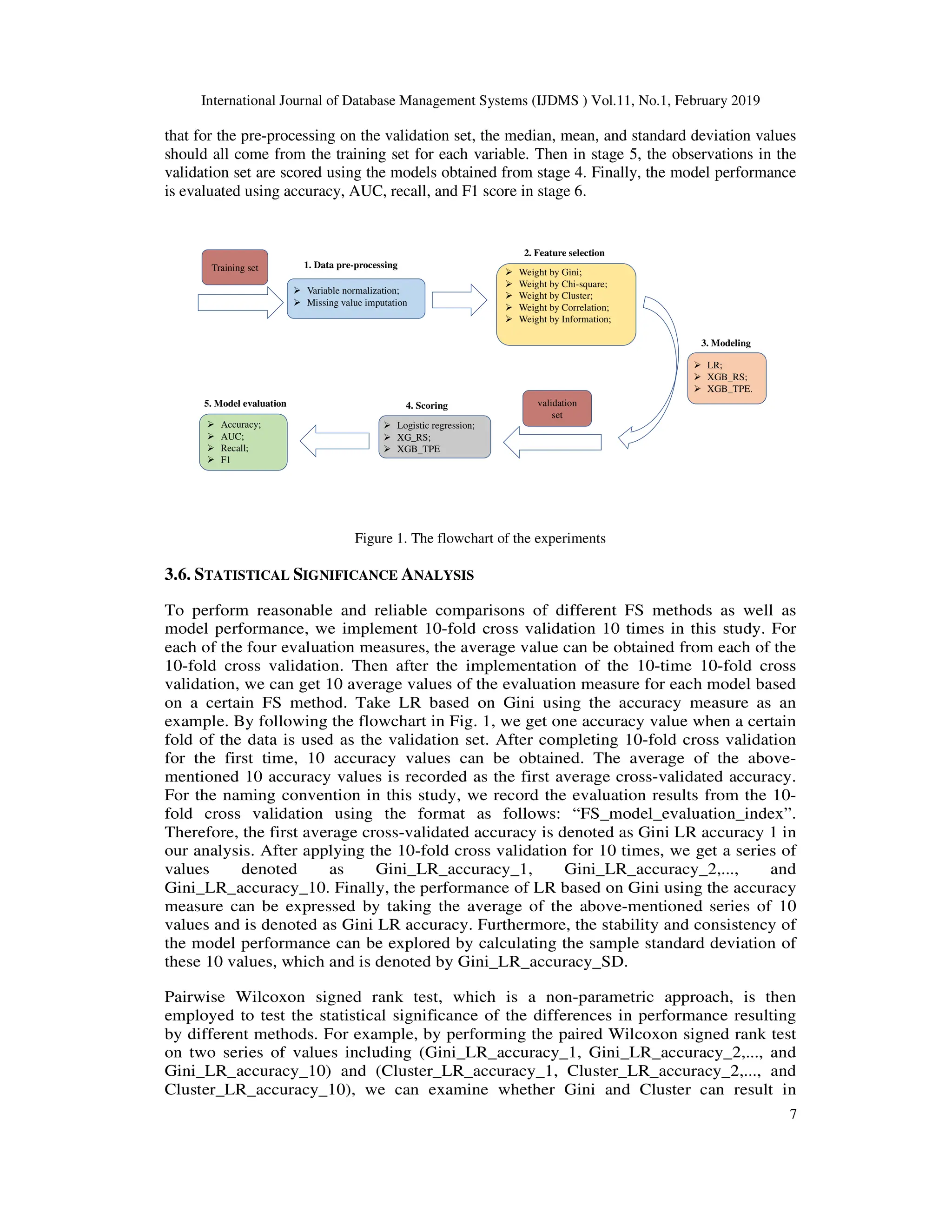
3.5. FLOWCHART OF THE EXPERIMENTS
After the data pre-processing procedures described in Section 3.2, the models are built on the
training set while the performance is evaluated on the validation set. To ensure the reliability and
accuracy of the results, we use 10-fold cross validation in this study. Fig.1 shows the flowchart of
the analysis where a certain fold of the data is used as the validation set while the rest of the nine
folds are used as the training set.As illustrated in Fig. 1, the entire analysis process contains six
stages. In stage 1, the training set is pre-processed following the steps below:
• For each feature in the training set, we performed missing value imputation using
itsmedian value;
• Normalization of the variables by transforming every variable to its z-score using its
mean and standard deviations in the training set.
In stage 2, five FS approaches including Gini, Chi-square, Cluster, Correlation, and Information
are applied on the training set. This can select the most representative subset of the features. To
make the comparison of the model performance based on different FS methods fair, we fix the
size of the subset of the features as 50. The reason why we select 50 features is illustrated in
Section 4.1. In stage 3, three models including LR, XGB_RS, and XGB_TPE are built using the
subset of the features produced by different FS methods from stage 2. In stage 4, the validation
set is pre-processed using similar strategies as that on the training set in stage 1. It is worth noting](https://image.slidesharecdn.com/11119ijdms01-250312052208-d221ec1a/75/A-Xgboost-Risk-Model-Via-Feature-Selection-and-Bayesian-Hyper-Parameter-Optimization-6-2048.jpg)
![International Journal of Database Management Systems (IJDMS ) Vol.11, No.1, February 2019
8
different accuracy in LR. By comparing the difference of the FS methods for each of the
three models, the optimal FS approach for each model can be identified. Then, the
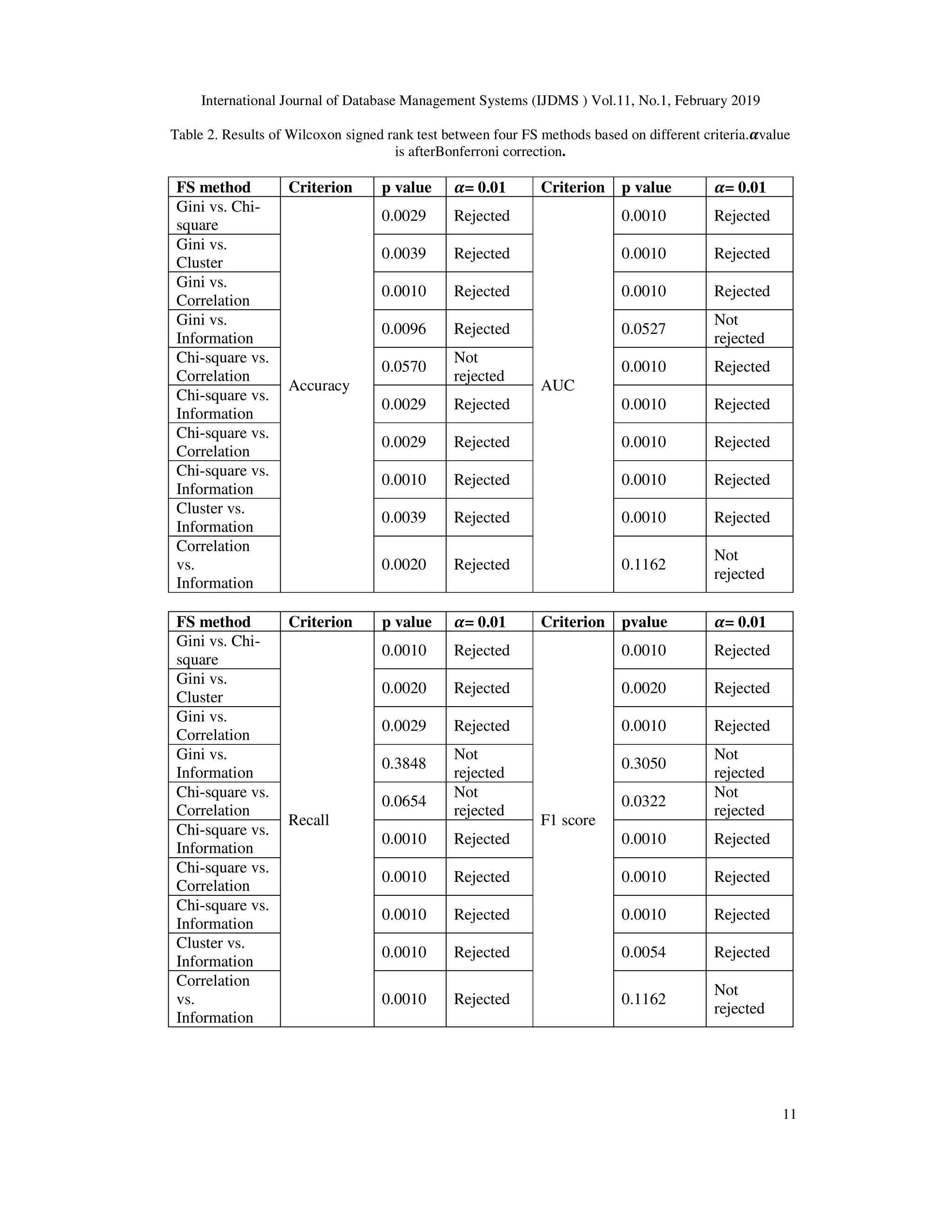
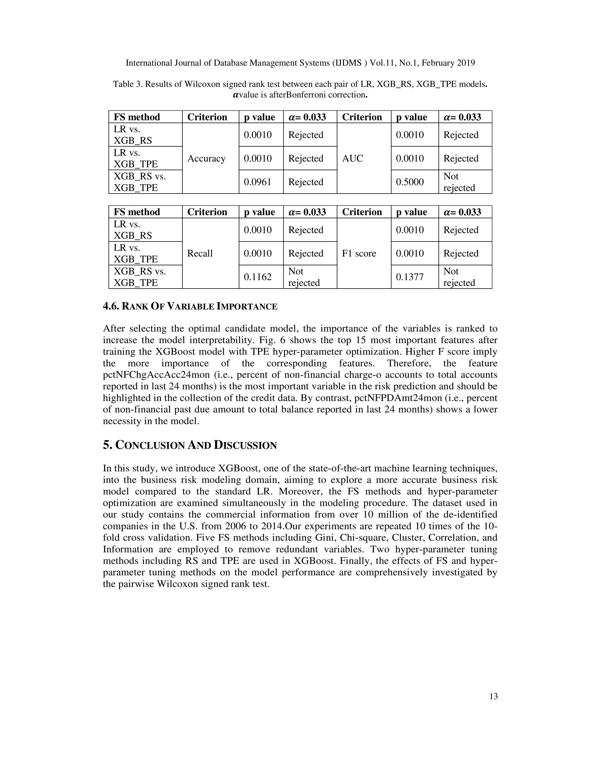
pairwise Wilcoxon signed rank test is used to compare different evaluation criteria of the
models comprehensively along with their optimal FS approach, thereby to select the
final optimal model. With respect to the desired significant level during the pairwise
comparison, it is set toα = 0.1 in this study. Bonferroni correction is used in this study to
handle the problem from theincreased Type I error by testing each individual
hypothesis[36]. As a result, each individual hypothesis is tested at the level α/m, where
m denotes the number of null hypothesis that are tested. For example, when comparing
the performance of LR, XGB_RS, and XGB_TPE, three individual tests are needed and
Bonferroni correction would test each individual hypothesis at α/3 = 0.033.
4. RESULTS
In this section, the effects of different FS methods on model performance are
demonstrated. Furthermore, Bayesian TPE hyper-parameter optimization on XGBoost is
compared with the RS method. With respect to the analysis tools in this study, SAS
(version 9.4) is used for data pre-processing that is labelled as stage 1 and 4 in Fig. 1.
The Cluster FS method is also implemented in SAS and the rest four FS methods are
implemented on RapidMiner (version 9.0). The training and scoring procedures of LR
are implemented on RapidMiner as well. XGB_TPE and XGB_RS are performed on
Python (version 3.5). All the experiments are operated on the desktop computer with
MacOS system, 3.3 GHz Intel Core I7 process, and 16GB RAM.
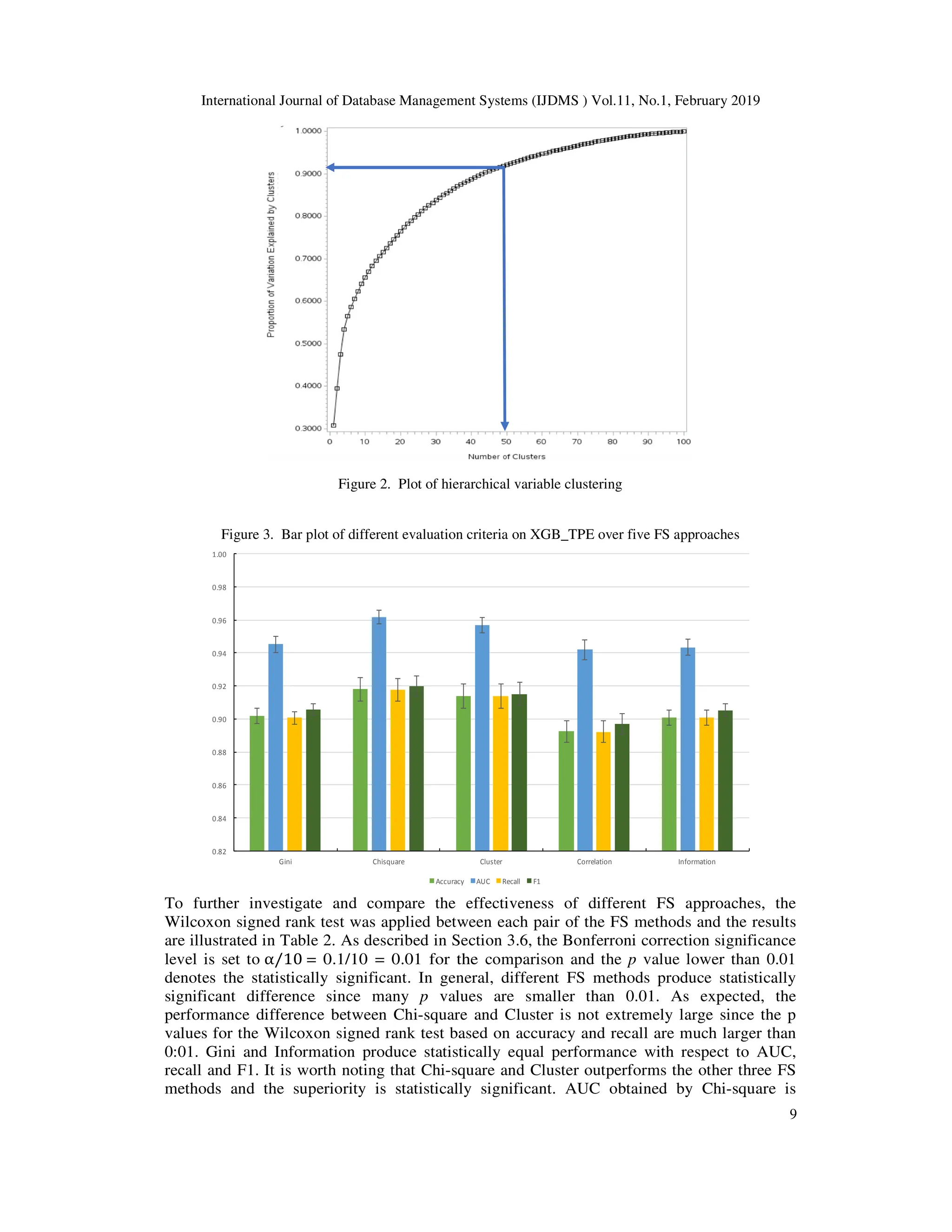
4.1. PARAMETER SETTINGS IN FS METHODS
In RapidMiner, one important parameter of FS that needs careful setting is “number of
features selected”. It is because too many features tend to hurt model performance due to
the potential multicollinearity problem while too few features may not capture enough
information based on the original dataset. In our study, the “number of features selected”
is determined based on the result from the Cluster FS method. As shown in Fig. 2, over
90% of the variations in the original dataset can be explained by 50 clusters. Therefore,
in the Cluster FS method, we select one representative feature from each of the 50
clusters and believe that enough information provided by the data can be kept. To ensure
the fair comparison among different FS methods, the value of “number of features
selected” is set to 50 for Gini, Chi-square, Correlation, and Information as well.
4.2. BEST FS METHOD IN XGB_TPE
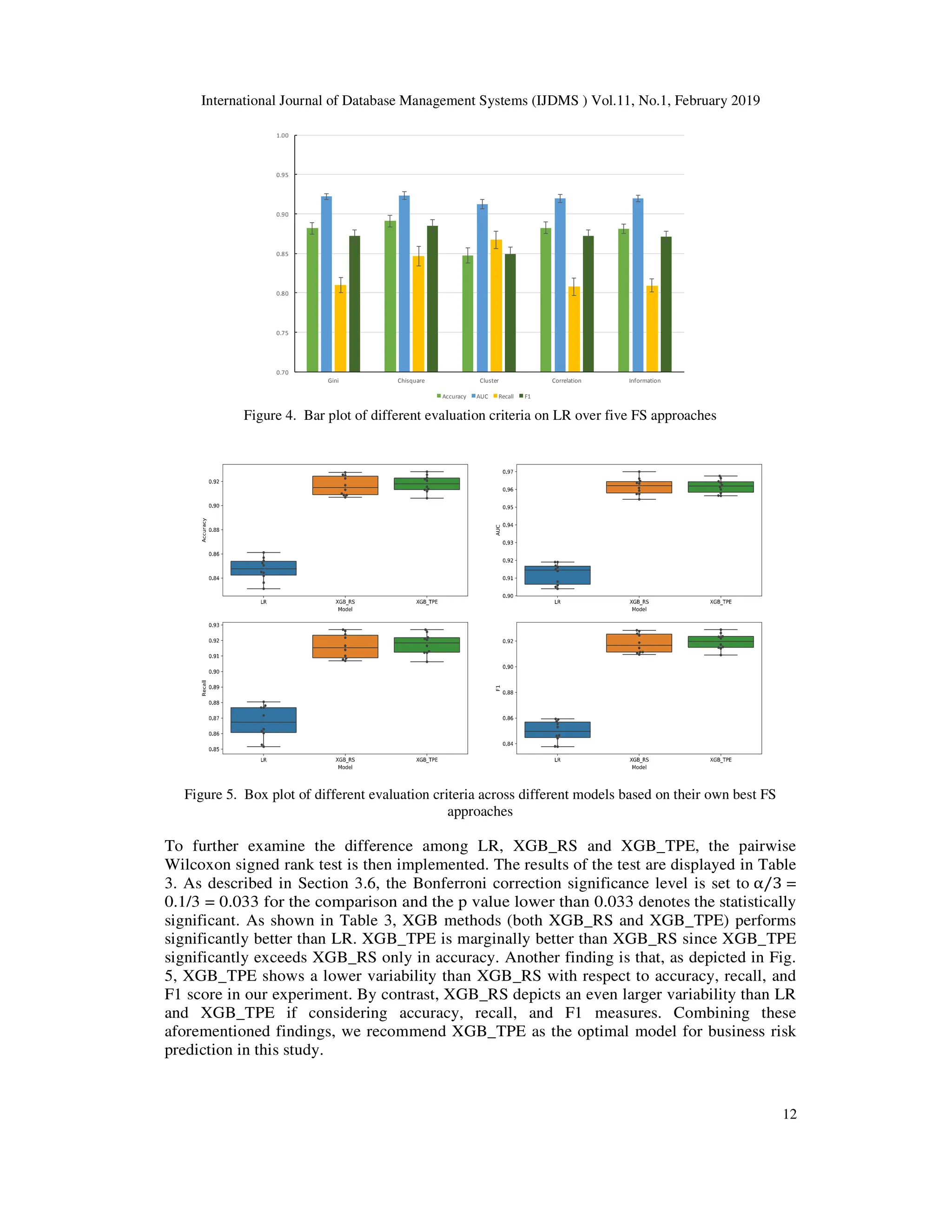
Fig. 3 demonstrated the XGB_TPE performance over five FS approaches by using the four
evaluation measures. As described in Section 3.6, the experiments were implemented using
10-fold cross validation and were repeated 10 times, the evaluation measures expressed in
Fig. 3 are the average cross-validated values along with the standard deviations. It is
observed that different FS approaches produce very different results. The Chi-square method
can achieve the highest accuracy, AUC, Recall and F1 score among the five FS methods. On
the other hand, Gini has the worst performance since it results in the lowest values in any of
the four evaluation criteria. There seems to be no obvious difference in the model
performance between Chi-square and Cluster. The above-mentioned two FS methods
outperform the rest three methods in all the evaluation measures. Moreover, the three FS
methods including Gini, Correlation, and Information do not result in obvious difference in
the model performance. Another finding is that, the small values of the standard deviations
show the consistency and stability of the FS methods on the XGB_TPE model.](https://image.slidesharecdn.com/11119ijdms01-250312052208-d221ec1a/75/A-Xgboost-Risk-Model-Via-Feature-Selection-and-Bayesian-Hyper-Parameter-Optimization-8-2048.jpg)
![International Journal of Database Management Systems (IJDMS ) Vol.11, No.1, February 2019
14
Figure 6. Top 15 most important features based on XGB_TPE model
Our analysis shows that the effect of FS methods on the model performance dependents on
the model type. In LR, Gini FS method can result in the lowest recall while it exhibits an
acceptable recall in XGB (both XGB_RS and XGB_TPE). Different FS methods result in
significant changes in AUC for XGB models but do not have obvious effect in LR. The
Cluster FS method is shown to be the optimal FS methods for LR while Chi-square
outperforms other FS methods in both XGB_RS and XGB_TPE. The comparisons with
traditional LR show the significant superiority of the XGBoost methods (both XGB_RS and
XGB_TPE) in terms of accuracy, AUC, recall and F1 score. Bayesian TPE hyper-parameter
optimization method is significantly better than RS hyper-parameter tuning, since XGB_TPE
achieves significantly higher accuracy than XGB_RS. Furthermore, XGB_TPE outperforms
XGB_RS in terms of AUC, re-call, and F1 score, although the improvements are not
statistically significant. It is also worth noting that XGB_TPE shows a lower variability than
XGB_RS by considering accuracy, recall, and F1 score. As the final result, we conclude that
XGB_TPE is marginally better than XGB_RS while significantly better than LR. Therefore,
XGB_TPE is selected as the optimal model for business risk modeling in our study. The
ranking of the variable importance shows that pctNFChgAccAcc24mon is the most
important variable in the risk predictions while the weight of pctNFPDAmt24mon is not
obvious in the final model. The result demonstrated in Fig. 6 can provide guidance to
financial institutes in the collection of credit data.
Besides the above-mentioned promising results achieved by XGBoost on risk modeling
using the medium sized data in this study, XGBoost has been demonstrated to be powerful in
handling large scale data using very limited computing resources [20]. According to the
experimental results in [20], XGBoostachieves scalable learning through parallel and
distributed computing, out-of-core computation, and cache-aware learning.When the real-
world data used in the risk modeling domain is large, the out-of-core computation in
XGBoost can utilize the disk space if the data is too large to fit into the main memory.
Therefore, XGBoost provides the insights for the data scientist on how to efficiently manage
and load large scale database using minimal amount of computing resources.
In the future business risk modeling studies, the results might not be consistent because of
using different dataset. However, the workflow proposed in our study may serve as a
reference for future studies in building XGBoost models and ranking variable importance in
the credit domain. This study can also provide a guidance for comprehensively exploring the
effect of FS algorithms as well as hyper-parameter optimization on the model performance.](https://image.slidesharecdn.com/11119ijdms01-250312052208-d221ec1a/75/A-Xgboost-Risk-Model-Via-Feature-Selection-and-Bayesian-Hyper-Parameter-Optimization-14-2048.jpg)
![International Journal of Database Management Systems (IJDMS ) Vol.11, No.1, February 2019
15
REFERENCES
[1] E. I. Altman and A. Saunders, "Credit risk measurement: Developments over the last 20
years,"Journal of banking &finance, vol. 21, no. 11-12, pp. 1721-1742, 1997.
[2] R. A. Walkling, "Predicting tender offer success: A logistic analysis,"Journal of financial and
Quantitative Analysis, vol. 20, no. 4, pp. 461-478, 1985.
[3] S. Finlay, "Multiple classifier architectures and their application to credit risk assessment," European
Journal of Operational Research, vol. 210, no. 2, pp. 368-378, 2011.
[4] Y. Wang and J. L. Priestley, “Binary classification on past due of service accounts using logistic
regression and decision tree,” 2017.
[5] Y. Wang, X. S. Ni, and B. Stone, "A two-stage hybrid model by using artificial neural networks as
feature construction algorithms," arXiv preprint arXiv:1812.02546, 2018.
[6] Y. Zhou, M. Han, L. Liu, J.S. He, and Y. Wang, "Deep learning approach for cyberattack
detection,"IEEE INFOCOM 2018-IEEE Conference on Computer Communications Workshops
(INFOCOM WKSHPS). IEEE, pp. 262-267, 2012.
[7] I. Brown and C. Mues, "An experimental comparison of classification algorithms for imbalanced
credit scoring data sets," Expert Systems with Applications, vol. 39, no. 3, pp. 3446-3453, 2012.
[8] G. Paleologo, A. Elisseeff, and G. Antonini, "Subagging for credit scoring models," European journal
of operational research, vol. 201, no. 2, pp. 490-499, 2010.
[9] G. Wang, J. Ma, L. Huang, and K. Xu, "Two credit scoring models based on dual strategy ensemble
trees," Knowledge-Based Systems, vol. 26, pp. 61-68, 2012.
[10] T. Chen, T. He, M. Benesty et al., "Xgboost: extreme gradient boosting," R pack-age version 0.4-2,
pp. 1{4, 2015.
[11] M. Zieba, S. K. Tomczak, and J. M. Tomczak, "Ensemble boosted trees with synthetic features
generation in application to bankruptcy prediction," Expert Systems with Applications, vol. 58, pp.
93-101, 2016.
[12] Y. Xia, C. Liu, Y. Li, and N. Liu, "A boosted decision tree approach using Bayesian hyper-parameter
optimization for credit scoring," Expert Systems with Applications, vol. 78, pp. 225-241, 2017.
[13] S. Piramuthu, "Evaluating feature selection methods for learning in data mining applications,"
European journal of operational research, vol. 156, no. 2, pp. 483-494, 2004.
[14] J. Bergstra and Y. Bengio, "Random search for hyper-parameter optimization," Journal of Machine
Learning Research, vol. 13, no. Feb, pp. 281-305, 2012.
[15] J. Bergstra, D. Yamins, and D. D. Cox, "Hyperopt: A python library for optimizing the
hyperparameters of machine learning algorithms," in Proceedings of the 12th Python in Science
Conference. Citeseer, 2013, pp. 13-20.
[16] F. N. Koutanaei, H. Sajedi, and M. Khanbabaei, "A hybrid data mining model of feature selection
algorithms and ensemble learning classifiers for credit scoring," Journal of Retailing and Consumer
Services, vol. 27, pp. 11-23, 2015.
[17] F. Akthar and C. Hahne, "RapidMiner 5 operator reference," Rapid-I GmbH, vol. 50, p. 65, 2012.
[18] R. Agrawal, J. Gehrke, D. Gunopulos, and P. Raghavan, Automatic subspace clustering of high
dimensional data for data mining applications. ACM, 1998, vol. 27, no. 2.
[19] S. Lessmann, B. Baesens, H.-V. Seow, and L. C. Thomas, "Benchmarking state-of-the-art
classification algorithms for credit scoring: An update of research," European Journal of Operational
Research, vol. 247, no. 1, pp. 124-136, 2015.
[20] T. Chen and C. Guestrin, "Xgboost: A scalable tree boosting system," in Proceedings of the 22nd
acmsigkdd international conference on knowledge discovery and data mining. ACM, 2016, pp. 785-
794.](https://image.slidesharecdn.com/11119ijdms01-250312052208-d221ec1a/75/A-Xgboost-Risk-Model-Via-Feature-Selection-and-Bayesian-Hyper-Parameter-Optimization-15-2048.jpg)
![International Journal of Database Management Systems (IJDMS ) Vol.11, No.1, February 2019
16
[21] L. Breiman, "Random forests," Machine learning, vol. 45, no. 1, pp. 5-32, 2001.
[22] J. S. Bergstra, R. Bardenet, Y. Bengio, and B. Kegl, "Algorithms for hyper-parameter optimization,"
in Advances in neural information processing systems, 2011, pp. 2546-2554.
[23] J. Bergstra, B. Komer, C. Eliasmith, D. Yamins, and D. D. Cox, "Hyperopt: a python library for
model selection and hyperparameter optimization," Computational Science & Discovery, vol. 8, no.
1, p. 014008, 2015.
[24] B. Shahriari, K. Swersky, Z. Wang, R. P. Adams, and N. De Freitas, "Taking the human out of the
loop: A review of Bayesian optimization," Proceedings of the IEEE, vol. 104, no. 1, pp. 148-175,
2016.
[25] J. Bergstra, D. Yamins, and D. D. Cox, "Making a science of model search: Hyper-parameter
optimization in hundreds of dimensions for vision architectures," 2013.
[26] C. Thornton, F. Hutter, H. H. Hoos, and K. Leyton-Brown, "Auto-weka: Combined selection and
hyperparameter optimization of classification algorithms," in Proceedings of the 19th ACM SIGKDD
international conference on Knowledge discovery and data mining. ACM, 2013, pp. 847-855.
[27] F. Hutter, H. H. Hoos, and K. Leyton-Brown, "Sequential model-based optimization for general
algorithm configuration," in International Conference on Learning and Intelligent Optimization.
Springer, 2011, pp. 507-523.
[28] L. Breiman, Classification and regression trees. Routledge, 2017.
[29] J. Elith, J. R. Leathwick, and T. Hastie, "A working guide to boosted regression trees," Journal of
Animal Ecology, vol. 77, no. 4, pp. 802-813, 2008.
[30] G. G. Moisen, E. A. Freeman, J. A. Blackard, T. S. Frescino, N. E. Zimmermann, and T. C. Edwards
Jr, "Predicting tree species presence and basal area in utah: a comparison of stochastic gradient
boosting, generalized additive models, and tree-based methods," Ecological modelling, vol. 199, no.
2, pp. 176-187, 2006.
[31] S. V. Stehman, "Selecting and interpreting measures of thematic classification accuracy," Remote
sensing of Environment, vol. 62, no. 1, pp. 77-89, 1997.
[32] E. A. Freeman and G. G. Moisen, "A comparison of the performance of threshold criteria for binary
classification in terms of predicted prevalence and kappa," Ecological Modelling, vol. 217, no. 1-2,
pp. 48-58, 2008.
[33] D. M. Powers, "Evaluation: from precision, recall and f-measure to roc, informedness, markedness
and correlation," 2011.
[34] S. Beguer a, "Validation and evaluation of predictive models in hazard assessment and risk
management," Natural Hazards, vol. 37, no. 3, pp. 315-329, 2006.
[35] Y. Sasaki et al., "The truth of the f-measure," Teach Tutor mater, vol. 1, no. 5, pp. 1-5, 2007.
[36] E. W. Weisstein, "Bonferroni correction," 2004.](https://image.slidesharecdn.com/11119ijdms01-250312052208-d221ec1a/75/A-Xgboost-Risk-Model-Via-Feature-Selection-and-Bayesian-Hyper-Parameter-Optimization-16-2048.jpg)

![International Journal of Database Management Systems (IJDMS ) Vol.11, No.1, February 2019
DOI : 10.5121/ijdms.2019.11101 1
A XGBOOST RISK MODEL VIA FEATURE
SELECTION AND BAYESIAN HYPER-PARAMETER
OPTIMIZATION
Yan Wang1
and Xuelei Sherry Ni2
1
Graduate College, Kennesaw State University, Kennesaw, USA
2
Department of Statistics and Analytical Sciences, Kennesaw State University,
Kennesaw, USA
ABSTRACT
This paper aims to explore models based on the extreme gradient boosting (XGBoost) approach for
business risk classification. Feature selection (FS) algorithms and hyper-parameter optimizations are
simultaneously considered during model training. The five most commonly used FS methods including
weight by Gini, weight by Chi-square, hierarchical variable clustering, weight by correlation, and weight
by information are applied to alleviate the effect of redundant features. Two hyper-parameter optimization
approaches, random search (RS) and Bayesian tree-structuredParzen Estimator (TPE), are applied in
XGBoost. The effect of different FS and hyper-parameter optimization methods on the model performance
are investigated by the Wilcoxon Signed Rank Test. The performance of XGBoost is compared to the
traditionally utilized logistic regression (LR) model in terms of classification accuracy, area under the
curve (AUC), recall, and F1 score obtained from the 10-fold cross validation. Results show that
hierarchical clustering is the optimal FS method for LR while weight by Chi-square achieves the best
performance in XG-Boost. Both TPE and RS optimization in XGBoost outperform LR significantly. TPE
optimization shows a superiority over RS since it results in a significantly higher accuracy and a
marginally higher AUC, recall and F1 score. Furthermore, XGBoost with TPE tuning shows a lower
variability than the RS method. Finally, the ranking of feature importance based on XGBoost enhances the
model interpretation. Therefore, XGBoost with Bayesian TPE hyper-parameter optimization serves as an
operative while powerful approach for business risk modeling.
KEYWORDS
Extreme gradient boosting; XGBoost; feature selection; Bayesian tree-structured Parzen estimator; risk
modeling
1. INTRODUCTION
Risk modeling is an effective tool to assist financial institutions to properly decide
whether or not to grant loans to business or other applicants [1]. Thereby, the problem of
risk modeling is transformed into a binary classification task, i.e., grant loans to low risk
applicants or not grant to those with high risk. Logistic regression (LR) is a traditionally
utilized technique for binary classificationsin the financial domain because of its easy
implementation, explainable results, as well as the similar and often better performance
compared to other binary classifiers such as decision trees and neural networks [2] [3]
[4] [5] [6]. On the other hand, it has been shown that a single classifier cannot solve all
problems effectively while ensemble models have been revealed to be promising in
many credit risk studies [7] [8] [9]. One of the state-of-the-art ensemble approach is the
extreme gradient boosting (XGBoost). It is a novel while advanced variant of the](https://crownmelresort.com/image.slidesharecdn.com/11119ijdms01-250312052208-d221ec1a/75/A-Xgboost-Risk-Model-Via-Feature-Selection-and-Bayesian-Hyper-Parameter-Optimization-1-2048.jpg)
![International Journal of Database Management Systems (IJDMS ) Vol.11, No.1, February 2019
2
gradient boosting algorithm and has obtained promising results in many Kaggle machine
learning competitions [10]. Furthermore, XGBoost has been successfully applied in
bankruptcy prediction and credit scoringin a few studies[11][12].
Numerous studies have focused on offering novel mechanisms to enhance the
performance of credit risk modeling. It has been demonstrated that feature selection (FS)
is one of the efficient approaches in improving model performance because of its ability
to alleviate the effects of noise and redundant variables [13]. Another method for model-
improving is the hyper-parameter optimization or tuning. It is shown that careful hyper-
parameter tuning tends to prevent the failure and reduce the over-fitting problem of
XGBoost. The two main strategies used for finding the proper setting of hyper-
parameters in XGBoost are random search (RS) and Bayesian tree-structured Parzen
estimator (TPE). They have demonstrated substantial influence on classification
performance [14] [15].
After careful paper review, we find that there is seldom research aiming at exploring the
effect of FS and hyper-parameter optimizations simultaneously on XGBoost in the
financial domain. Therefore, motivated by the aforementioned studies, we set up a series
of experiments that contain FS methods and hyper-parameter optimizations
simultaneously, thereby exploring an accurate and comprehensive business risk model
based on XGBoost. The superiority of XGBoost over the widely used LR is evaluated
via classification accuracy, area under the curve (AUC), recall, and F1 score. Moreover,
the effect of different FS as well as hyper-parameter optimization methods on the model
performance is comprehensively investigated through the Wilcoxon signed rank test.
Finally, the features are ranked according to their importance score to enhance the model
interpretation.
This paper has been structured as follows. Since different FS methods and XGBoost
models along with the hyper-parameter optimization are used in this study, we will first
describe the relevant algorithms in Section 2. Then the experimental design is discussed
in Section 3. Section 4 demonstrates the experimental results and discussions.Finally,
Section 5 addresses the conclusions.
2. ALGORITHMS
In this section, the algorithms related to FS and XGBoost along with hyper-parameter
optimizations are discussed.
2.1. FEATURE SELECTION METHODS
FS methods aims to filter the redundant variables and select the most appropriate subset of
features. By applying FS methods to the dataset, we can decrease the effect of the noise as
well as reduce the computational cost during the modeling stage. Many studies have shown
that FS can be used to increase the classification performance [13] [16].
In this study, five commonly used FS methods are applied and evaluated: weight by gini
index, weight by chi-square, hierarchical variable clustering, weight by correlation, and
weight by information gain ratio. For simplicity, we use the terms with initial capitalization
to denote different FS methods. Therefore, Gini, Chi-square, Cluster, Correlation, and
Information are used to represent the aforementioned five FS approaches, respectively. In the
Gini FS method, the value of an attribute is evaluated via the gini impurity index. Similarly,
Chi-square, Correlation, and Information evaluates the relevance of the feature by calculating
its chi-squared statistic, correlation, and information gain ratio with respect to the target
variable [17]. Features with higher values of gini index, chi-squared statistic, correlation, and](https://crownmelresort.com/image.slidesharecdn.com/11119ijdms01-250312052208-d221ec1a/75/A-Xgboost-Risk-Model-Via-Feature-Selection-and-Bayesian-Hyper-Parameter-Optimization-2-2048.jpg)
![International Journal of Database Management Systems (IJDMS ) Vol.11, No.1, February 2019
3
information gain ratio are selected in the FS results. On the other hand, the Cluster method
bases on the variable clustering analysis and selects the best feature within each cluster
according to the 1-R2
ratio defined in Eq. 1 [18]. Different from the rest of the four FS
methods, features with lower 1-R2
ratio are selected by the Cluster method.
1 − =
1 − _
1 − _ _
(1)
2.2. LOGISTIC REGRESSION
LR is a standard binary classification technique widely used in industry because of its
simplicity and balanced error distribution [19] [21]. It outputs the conditional probability p of
an observation that belongs to a specific class using the formula defined in Eq. 2, where ( ,
, ..., ) denotes the input variables while ( . . . , ) represents the unknown parameters
that need to be estimated.
p =
exp ( + ∗ + ∗ + ⋯ + ∗ )
1 + exp ( + ∗ + ∗ + ⋯ + ∗ )
( (2)
2.3. EXTREME GRADIENT BOOSTING ALONG WITH HYPER-PARAMETERS
XGBoost was proposed in 2015 and has been frequently applied because of its rapidness,
efficiency, and scalability [10]. It is an advanced implementation ofthe gradient boosting
(GB) algorithm and uses the decision tree as the base classifier. After carefully reading the
research in [12] and [20], the algorithm of GB and XGBoost is briefly summarized as
follows. Suppose we have a dataset D = {); *} containing n observations, where )and
*denotes the features and the target variable, respectively. In GB, suppose there are K
number of boosting, then we use B additive functions to predict the output. Denote +
,- as the
prediction for the -th instance at the .-th boost, /0 represents a tree structure q with leaf j
having a weight score 12. Then for a given instance -, the final prediction is calculated by
summing up the scores across all leaves and this can be expressed in Eq. 3.
+
,- = 3 /0(
4
05
-)
(3)
The idea of GB is to minimize the loss function 60 defined using Eq. 4, where l(+-, +
,- )
measures the difference between the prediction and its real value +-. Since the base learner of
GB is decision tree, several hyper-parameters related to the tree structures including
subsample, max leaves, and max depth are employed to reduce the over-fitting problem as
well as to enhance the model. Moreover, learning rate or the shrinkage factor, which controls
the weighting of new trees added to the model, is also used to decrease the rate of the
model’sadaptation to the training data. The above-mentioned hyper-parameters are also
defined in XGBoost and their descriptions can be found in Table 1.
60 = 3 7(+-,
-5
+
,- ) (4)
By adding a regularization term 8(/0) to the loss function defined in Eq. 4, we can get the
loss function of XGB described in Eq. 5, The regularization term 8(/0)penalizes the model
complexity. It can be expressed by summing up two parts: 9: and 0.5=||1|| . :representsthe](https://crownmelresort.com/image.slidesharecdn.com/11119ijdms01-250312052208-d221ec1a/75/A-Xgboost-Risk-Model-Via-Feature-Selection-and-Bayesian-Hyper-Parameter-Optimization-3-2048.jpg)
![International Journal of Database Management Systems (IJDMS ) Vol.11, No.1, February 2019
4
number of leaves that are contained by the tree. The hyper-parameter 9defines the minimum
loss reduction for further partition. If the loss reduction is less than 9, XGBoost stops,
implying that penalizes the model complexity.= is a fixed coefficient and ||1|| represents
the L2 norm of the weight of the leaf.Similar to 9, a hyper-parameter 1? controls the tree
depth and a substantial 1? makes the model more conservative in splitting. 1? is defined
as the minimum sum of the in-stance weight in further partitioning. The descriptions of the
above-mentioned hyper-parameters can be found in Table 1.
60 = 3 7(+-,
-5
+
,- ) + 3 8(/0)
4
05
= 3 7(+-,
-5
+
,- ) + 9: + 0.5=||1|| (5)
Compared with GB, another technique used in XGBoost for the further prevention of over-
fitting is the column subsampling or feature subsampling [11]. It is shown that using column
subsampling is even more efficient than traditional row subsampling in preventing over-
fitting [14]. The description of the corresponding hyper-parameter “colsample_bytree” can
be found in Table 1.
2.4. HYPER-PARAMETER OPTIMIZATION METHODS IN XGBOOST
In XGB, hyper-parameter optimization (i.e., tuning) aims at searching for the hyper-
parameter values that minimizes the objective function defined in Eq. 5. There are two
popular hyper-parameter optimization methods: RS and Bayesian Tree Parzen Estimators
(TPE). RS means the hyper-parameters are randomly picked from the pre-defined searching
domain uniformly and the searching does not depend onthe previous boosting result [14]
[22]. It has been shown to be efficient for problems with high dimensions in some studies.
On the contrary, Sequential Model Based Optimization (SMBO), which is also named
Bayesian optimization, is a probability based approach and uses the probability model to
select the most promising hyper-parameters [23]. According to the choices of the probability
model (i.e., the surrogate model), several variants of SMBO are proposed including Gaussian
Processes, Random Forest Regressions, and TPE [24] [25]. Since several studies have
revealed the promising results via TPE approach, we adopt this method in our study [26]
[27]. For simplicity, in the rest of the paper, we use XGB_TPE and XGB_RS to denote the
XGBoost models built by using Bayesian TPE and RS hyper-parameter optimization
methods, respectively.
3. EXPERIMENTAL DESIGN
In this study, we aim to answer the following four research questions explicitly based on the
dataset used:
• How different FS methods affect the performance of LR and XGBoost? What is the
corresponding optimal FS method for different models?
• How the hyper-parameter optimization methods including RS and TPE affect the
performance of XGBoost?
• Is the XGBoost method more powerful in business risk prediction compared to
traditionally utilized LR?
• Based on the dataset used in this study, what are the important features in the risk
prediction?](https://crownmelresort.com/image.slidesharecdn.com/11119ijdms01-250312052208-d221ec1a/75/A-Xgboost-Risk-Model-Via-Feature-Selection-and-Bayesian-Hyper-Parameter-Optimization-4-2048.jpg)
![International Journal of Database Management Systems (IJDMS ) Vol.11, No.1, February 2019
5
To address the above-mentioned questions, a comprehensive experimental study is
conducted and the details are described in the following subsections.
3.1. DATA DESCRIPTION
The dataset used in this study is contributed by a national credit bureau and contains over 10
million de-identified commercial information of the companies in the U.S. from 2006 to
2014. The 305 independent variables are all numeric and provide information of the
companies' activities in non-financial accounts, telecommunication accounts, and industry
accounts, etc. The dependent variable RiskFlag represents whether the business is in risk or
not. The positive rate (i.e., proportion of risky business) in the dataset is about 52%.
3.2. DATA PRE-PROCESSING
Based on the original dataset, we first replaced the invalid records of variables with missing
values and then removed the variables with missing percentage larger than 70%. As the
result, out of the 305 independent variables, 108 variables are kept in our study. Then a
stratified sampling procedure was applied to obtain a sample with 8000 observations for the
further experiments described in this Section.
3.3. SEARCHING DOMAIN OF HYPER-PARAMETERS IN XGBOOST
As discussed in Sections 2.3 and 2.4, several hyper-parameters of XGBoost needs to be
optimized based on a pre-defined domain using RS and Bayesian TPE methods to avoid the
over-fitting in this study. Although many hyper-parameters are included in XGBoost, we
only focus on those that are shown to have significant effect on the model performance in the
previous studies. The hyper-parameters adopted in this study include “learning rate”,
“subsample”, “max_leaves”, “max_depth”, “gamma”, “colsample_bytree”, and
“min_child_weight”.The corresponding searching domain and the descriptions of the hyper-
parameters are summarized in Table 1. The settings of the searching domain are based on the
suggestions from previous research as well as based on our initial trials [28] [29] [30]. For
the rest of other hyper-parameters including “n_estimators” (number of boosted trees),
“min_child_samples” (minimum number of data needed in a leaf) and “subsample_for_bin”
(number of samples for constructing bins), we use the default settings in Python [20].
3.4. PERFORMANCE EVALUATION CRITERIA
The criteria used to evaluate the model performance are discussed in this section.
Accuracy is the commonly used measure in binary classification problems and can
provide reasonable model comparisons [31]. In this study, True Positive (TP) and False
Positive (FP) represent correctly and wrongly classified risky businesses, respectively.
True Negative (TN) and False Negative (FN) denote correctly and wrongly classified
non-risky businesses, respectively. Then accuracy can be calculated using Eq. 6. Another
evaluation measure used, AUC, is the area under the Receiver Operating Characteristic
Curve (ROC) since it measures how well the model distinguishes the positives and the
negatives [32]. ROC is plotted by using false positive rate (i.e.,
@A
@ABCD
) on the x-axis and
true positive rate (i.e.,
CA
CAB@D
) on the y-axis. Recall (i.e., true positive rate) measuresthe
fraction of positives that have been retrieved over the total amount of all the positives
(defined in Eq. 7) while precision denotes the fraction of positives among the retrieved
positives [33] (defined in Eq. 8). As discussed in [34], recall and precision are
emphasized differently in risk modeling and hazard research domain. Similarly, in our
study, recall is weighted more heavily than precision since a false negative error may](https://crownmelresort.com/image.slidesharecdn.com/11119ijdms01-250312052208-d221ec1a/75/A-Xgboost-Risk-Model-Via-Feature-Selection-and-Bayesian-Hyper-Parameter-Optimization-5-2048.jpg)
![International Journal of Database Management Systems (IJDMS ) Vol.11, No.1, February 2019
6
signify the loss. F1 score (defined in Eq. 9) is another model evaluation measure in this
paper since it is the harmonic mean of precision and recall [35].
Table 1. Searching domain of hyper-parameters in XGBoost. Hyper-parameters in bold are those that are
defined only in XGBoost but not in GB.
Name Description Domain
learning rate Step size shrinkage used in model update (0.005, 0.2)
subsample
Subsample ratio of the training instances used for
fitting the individual tree
(0.8, 1)
max_leaves Maximum number of nodes to be added (10, 200)
max_depth Maximum depth of a tree (5, 30)
gamma (E) Minimum loss reduction required for further partition (0, 0.02)
colsample_bytree
Subsample ratio of features/columnsused for fitting the
individual tree
(0.8, 1)
min_child_weight
(FGH)
Minimum weights of the instances required in a leaf (0, 10)
accuracy =
:N + :O
:N + :O + PN + PO
(6)
recall =
:N
:N + PO
(7)
precision =
:N
:N + PN
(8)
F1 score =
2 ∗ X YZ [ ∗ YZ 77
X YZ [ + YZ 77
(9)
3.5. FLOWCHART OF THE EXPERIMENTS
After the data pre-processing procedures described in Section 3.2, the models are built on the
training set while the performance is evaluated on the validation set. To ensure the reliability and
accuracy of the results, we use 10-fold cross validation in this study. Fig.1 shows the flowchart of
the analysis where a certain fold of the data is used as the validation set while the rest of the nine
folds are used as the training set.As illustrated in Fig. 1, the entire analysis process contains six
stages. In stage 1, the training set is pre-processed following the steps below:
• For each feature in the training set, we performed missing value imputation using
itsmedian value;
• Normalization of the variables by transforming every variable to its z-score using its
mean and standard deviations in the training set.
In stage 2, five FS approaches including Gini, Chi-square, Cluster, Correlation, and Information
are applied on the training set. This can select the most representative subset of the features. To
make the comparison of the model performance based on different FS methods fair, we fix the
size of the subset of the features as 50. The reason why we select 50 features is illustrated in
Section 4.1. In stage 3, three models including LR, XGB_RS, and XGB_TPE are built using the
subset of the features produced by different FS methods from stage 2. In stage 4, the validation
set is pre-processed using similar strategies as that on the training set in stage 1. It is worth noting](https://crownmelresort.com/image.slidesharecdn.com/11119ijdms01-250312052208-d221ec1a/75/A-Xgboost-Risk-Model-Via-Feature-Selection-and-Bayesian-Hyper-Parameter-Optimization-6-2048.jpg)

![International Journal of Database Management Systems (IJDMS ) Vol.11, No.1, February 2019
8
different accuracy in LR. By comparing the difference of the FS methods for each of the
three models, the optimal FS approach for each model can be identified. Then, the
pairwise Wilcoxon signed rank test is used to compare different evaluation criteria of the
models comprehensively along with their optimal FS approach, thereby to select the
final optimal model. With respect to the desired significant level during the pairwise
comparison, it is set toα = 0.1 in this study. Bonferroni correction is used in this study to
handle the problem from theincreased Type I error by testing each individual
hypothesis[36]. As a result, each individual hypothesis is tested at the level α/m, where
m denotes the number of null hypothesis that are tested. For example, when comparing
the performance of LR, XGB_RS, and XGB_TPE, three individual tests are needed and
Bonferroni correction would test each individual hypothesis at α/3 = 0.033.
4. RESULTS
In this section, the effects of different FS methods on model performance are
demonstrated. Furthermore, Bayesian TPE hyper-parameter optimization on XGBoost is
compared with the RS method. With respect to the analysis tools in this study, SAS
(version 9.4) is used for data pre-processing that is labelled as stage 1 and 4 in Fig. 1.
The Cluster FS method is also implemented in SAS and the rest four FS methods are
implemented on RapidMiner (version 9.0). The training and scoring procedures of LR
are implemented on RapidMiner as well. XGB_TPE and XGB_RS are performed on
Python (version 3.5). All the experiments are operated on the desktop computer with
MacOS system, 3.3 GHz Intel Core I7 process, and 16GB RAM.
4.1. PARAMETER SETTINGS IN FS METHODS
In RapidMiner, one important parameter of FS that needs careful setting is “number of
features selected”. It is because too many features tend to hurt model performance due to
the potential multicollinearity problem while too few features may not capture enough
information based on the original dataset. In our study, the “number of features selected”
is determined based on the result from the Cluster FS method. As shown in Fig. 2, over
90% of the variations in the original dataset can be explained by 50 clusters. Therefore,
in the Cluster FS method, we select one representative feature from each of the 50
clusters and believe that enough information provided by the data can be kept. To ensure
the fair comparison among different FS methods, the value of “number of features
selected” is set to 50 for Gini, Chi-square, Correlation, and Information as well.
4.2. BEST FS METHOD IN XGB_TPE
Fig. 3 demonstrated the XGB_TPE performance over five FS approaches by using the four
evaluation measures. As described in Section 3.6, the experiments were implemented using
10-fold cross validation and were repeated 10 times, the evaluation measures expressed in
Fig. 3 are the average cross-validated values along with the standard deviations. It is
observed that different FS approaches produce very different results. The Chi-square method
can achieve the highest accuracy, AUC, Recall and F1 score among the five FS methods. On
the other hand, Gini has the worst performance since it results in the lowest values in any of
the four evaluation criteria. There seems to be no obvious difference in the model
performance between Chi-square and Cluster. The above-mentioned two FS methods
outperform the rest three methods in all the evaluation measures. Moreover, the three FS
methods including Gini, Correlation, and Information do not result in obvious difference in
the model performance. Another finding is that, the small values of the standard deviations
show the consistency and stability of the FS methods on the XGB_TPE model.](https://crownmelresort.com/image.slidesharecdn.com/11119ijdms01-250312052208-d221ec1a/75/A-Xgboost-Risk-Model-Via-Feature-Selection-and-Bayesian-Hyper-Parameter-Optimization-8-2048.jpg)


![International Journal of Database Management Systems (IJDMS ) Vol.11, No.1, February 2019
14
Figure 6. Top 15 most important features based on XGB_TPE model
Our analysis shows that the effect of FS methods on the model performance dependents on
the model type. In LR, Gini FS method can result in the lowest recall while it exhibits an
acceptable recall in XGB (both XGB_RS and XGB_TPE). Different FS methods result in
significant changes in AUC for XGB models but do not have obvious effect in LR. The
Cluster FS method is shown to be the optimal FS methods for LR while Chi-square
outperforms other FS methods in both XGB_RS and XGB_TPE. The comparisons with
traditional LR show the significant superiority of the XGBoost methods (both XGB_RS and
XGB_TPE) in terms of accuracy, AUC, recall and F1 score. Bayesian TPE hyper-parameter
optimization method is significantly better than RS hyper-parameter tuning, since XGB_TPE
achieves significantly higher accuracy than XGB_RS. Furthermore, XGB_TPE outperforms
XGB_RS in terms of AUC, re-call, and F1 score, although the improvements are not
statistically significant. It is also worth noting that XGB_TPE shows a lower variability than
XGB_RS by considering accuracy, recall, and F1 score. As the final result, we conclude that
XGB_TPE is marginally better than XGB_RS while significantly better than LR. Therefore,
XGB_TPE is selected as the optimal model for business risk modeling in our study. The
ranking of the variable importance shows that pctNFChgAccAcc24mon is the most
important variable in the risk predictions while the weight of pctNFPDAmt24mon is not
obvious in the final model. The result demonstrated in Fig. 6 can provide guidance to
financial institutes in the collection of credit data.
Besides the above-mentioned promising results achieved by XGBoost on risk modeling
using the medium sized data in this study, XGBoost has been demonstrated to be powerful in
handling large scale data using very limited computing resources [20]. According to the
experimental results in [20], XGBoostachieves scalable learning through parallel and
distributed computing, out-of-core computation, and cache-aware learning.When the real-
world data used in the risk modeling domain is large, the out-of-core computation in
XGBoost can utilize the disk space if the data is too large to fit into the main memory.
Therefore, XGBoost provides the insights for the data scientist on how to efficiently manage
and load large scale database using minimal amount of computing resources.
In the future business risk modeling studies, the results might not be consistent because of
using different dataset. However, the workflow proposed in our study may serve as a
reference for future studies in building XGBoost models and ranking variable importance in
the credit domain. This study can also provide a guidance for comprehensively exploring the
effect of FS algorithms as well as hyper-parameter optimization on the model performance.](https://crownmelresort.com/image.slidesharecdn.com/11119ijdms01-250312052208-d221ec1a/75/A-Xgboost-Risk-Model-Via-Feature-Selection-and-Bayesian-Hyper-Parameter-Optimization-14-2048.jpg)
![International Journal of Database Management Systems (IJDMS ) Vol.11, No.1, February 2019
15
REFERENCES
[1] E. I. Altman and A. Saunders, "Credit risk measurement: Developments over the last 20
years,"Journal of banking &finance, vol. 21, no. 11-12, pp. 1721-1742, 1997.
[2] R. A. Walkling, "Predicting tender offer success: A logistic analysis,"Journal of financial and
Quantitative Analysis, vol. 20, no. 4, pp. 461-478, 1985.
[3] S. Finlay, "Multiple classifier architectures and their application to credit risk assessment," European
Journal of Operational Research, vol. 210, no. 2, pp. 368-378, 2011.
[4] Y. Wang and J. L. Priestley, “Binary classification on past due of service accounts using logistic
regression and decision tree,” 2017.
[5] Y. Wang, X. S. Ni, and B. Stone, "A two-stage hybrid model by using artificial neural networks as
feature construction algorithms," arXiv preprint arXiv:1812.02546, 2018.
[6] Y. Zhou, M. Han, L. Liu, J.S. He, and Y. Wang, "Deep learning approach for cyberattack
detection,"IEEE INFOCOM 2018-IEEE Conference on Computer Communications Workshops
(INFOCOM WKSHPS). IEEE, pp. 262-267, 2012.
[7] I. Brown and C. Mues, "An experimental comparison of classification algorithms for imbalanced
credit scoring data sets," Expert Systems with Applications, vol. 39, no. 3, pp. 3446-3453, 2012.
[8] G. Paleologo, A. Elisseeff, and G. Antonini, "Subagging for credit scoring models," European journal
of operational research, vol. 201, no. 2, pp. 490-499, 2010.
[9] G. Wang, J. Ma, L. Huang, and K. Xu, "Two credit scoring models based on dual strategy ensemble
trees," Knowledge-Based Systems, vol. 26, pp. 61-68, 2012.
[10] T. Chen, T. He, M. Benesty et al., "Xgboost: extreme gradient boosting," R pack-age version 0.4-2,
pp. 1{4, 2015.
[11] M. Zieba, S. K. Tomczak, and J. M. Tomczak, "Ensemble boosted trees with synthetic features
generation in application to bankruptcy prediction," Expert Systems with Applications, vol. 58, pp.
93-101, 2016.
[12] Y. Xia, C. Liu, Y. Li, and N. Liu, "A boosted decision tree approach using Bayesian hyper-parameter
optimization for credit scoring," Expert Systems with Applications, vol. 78, pp. 225-241, 2017.
[13] S. Piramuthu, "Evaluating feature selection methods for learning in data mining applications,"
European journal of operational research, vol. 156, no. 2, pp. 483-494, 2004.
[14] J. Bergstra and Y. Bengio, "Random search for hyper-parameter optimization," Journal of Machine
Learning Research, vol. 13, no. Feb, pp. 281-305, 2012.
[15] J. Bergstra, D. Yamins, and D. D. Cox, "Hyperopt: A python library for optimizing the
hyperparameters of machine learning algorithms," in Proceedings of the 12th Python in Science
Conference. Citeseer, 2013, pp. 13-20.
[16] F. N. Koutanaei, H. Sajedi, and M. Khanbabaei, "A hybrid data mining model of feature selection
algorithms and ensemble learning classifiers for credit scoring," Journal of Retailing and Consumer
Services, vol. 27, pp. 11-23, 2015.
[17] F. Akthar and C. Hahne, "RapidMiner 5 operator reference," Rapid-I GmbH, vol. 50, p. 65, 2012.
[18] R. Agrawal, J. Gehrke, D. Gunopulos, and P. Raghavan, Automatic subspace clustering of high
dimensional data for data mining applications. ACM, 1998, vol. 27, no. 2.
[19] S. Lessmann, B. Baesens, H.-V. Seow, and L. C. Thomas, "Benchmarking state-of-the-art
classification algorithms for credit scoring: An update of research," European Journal of Operational
Research, vol. 247, no. 1, pp. 124-136, 2015.
[20] T. Chen and C. Guestrin, "Xgboost: A scalable tree boosting system," in Proceedings of the 22nd
acmsigkdd international conference on knowledge discovery and data mining. ACM, 2016, pp. 785-
794.](https://crownmelresort.com/image.slidesharecdn.com/11119ijdms01-250312052208-d221ec1a/75/A-Xgboost-Risk-Model-Via-Feature-Selection-and-Bayesian-Hyper-Parameter-Optimization-15-2048.jpg)
![International Journal of Database Management Systems (IJDMS ) Vol.11, No.1, February 2019
16
[21] L. Breiman, "Random forests," Machine learning, vol. 45, no. 1, pp. 5-32, 2001.
[22] J. S. Bergstra, R. Bardenet, Y. Bengio, and B. Kegl, "Algorithms for hyper-parameter optimization,"
in Advances in neural information processing systems, 2011, pp. 2546-2554.
[23] J. Bergstra, B. Komer, C. Eliasmith, D. Yamins, and D. D. Cox, "Hyperopt: a python library for
model selection and hyperparameter optimization," Computational Science & Discovery, vol. 8, no.
1, p. 014008, 2015.
[24] B. Shahriari, K. Swersky, Z. Wang, R. P. Adams, and N. De Freitas, "Taking the human out of the
loop: A review of Bayesian optimization," Proceedings of the IEEE, vol. 104, no. 1, pp. 148-175,
2016.
[25] J. Bergstra, D. Yamins, and D. D. Cox, "Making a science of model search: Hyper-parameter
optimization in hundreds of dimensions for vision architectures," 2013.
[26] C. Thornton, F. Hutter, H. H. Hoos, and K. Leyton-Brown, "Auto-weka: Combined selection and
hyperparameter optimization of classification algorithms," in Proceedings of the 19th ACM SIGKDD
international conference on Knowledge discovery and data mining. ACM, 2013, pp. 847-855.
[27] F. Hutter, H. H. Hoos, and K. Leyton-Brown, "Sequential model-based optimization for general
algorithm configuration," in International Conference on Learning and Intelligent Optimization.
Springer, 2011, pp. 507-523.
[28] L. Breiman, Classification and regression trees. Routledge, 2017.
[29] J. Elith, J. R. Leathwick, and T. Hastie, "A working guide to boosted regression trees," Journal of
Animal Ecology, vol. 77, no. 4, pp. 802-813, 2008.
[30] G. G. Moisen, E. A. Freeman, J. A. Blackard, T. S. Frescino, N. E. Zimmermann, and T. C. Edwards
Jr, "Predicting tree species presence and basal area in utah: a comparison of stochastic gradient
boosting, generalized additive models, and tree-based methods," Ecological modelling, vol. 199, no.
2, pp. 176-187, 2006.
[31] S. V. Stehman, "Selecting and interpreting measures of thematic classification accuracy," Remote
sensing of Environment, vol. 62, no. 1, pp. 77-89, 1997.
[32] E. A. Freeman and G. G. Moisen, "A comparison of the performance of threshold criteria for binary
classification in terms of predicted prevalence and kappa," Ecological Modelling, vol. 217, no. 1-2,
pp. 48-58, 2008.
[33] D. M. Powers, "Evaluation: from precision, recall and f-measure to roc, informedness, markedness
and correlation," 2011.
[34] S. Beguer a, "Validation and evaluation of predictive models in hazard assessment and risk
management," Natural Hazards, vol. 37, no. 3, pp. 315-329, 2006.
[35] Y. Sasaki et al., "The truth of the f-measure," Teach Tutor mater, vol. 1, no. 5, pp. 1-5, 2007.
[36] E. W. Weisstein, "Bonferroni correction," 2004.](https://crownmelresort.com/image.slidesharecdn.com/11119ijdms01-250312052208-d221ec1a/75/A-Xgboost-Risk-Model-Via-Feature-Selection-and-Bayesian-Hyper-Parameter-Optimization-16-2048.jpg)