Download as PDF, PPTX
![Instroduction
The world relies on software heavily now so it
should be reliable
Software Reliability is the probability of a
software system or component to perform its
intended function under the specified
operating conditions over the specified period
of time [1]
In other words the less faults there are in a
software the more reliable it is.](https://image.slidesharecdn.com/asurveyoffaultpredictionusingmachinelearningalgorithms-120226104850-phpapp02/75/A-survey-of-fault-prediction-using-machine-learning-algorithms-2-2048.jpg)
![[1]
A Fuzzy Model for Early Software
Fault Prediction Using Process
Maturity and Software Metrics](https://image.slidesharecdn.com/asurveyoffaultpredictionusingmachinelearningalgorithms-120226104850-phpapp02/75/A-survey-of-fault-prediction-using-machine-learning-algorithms-4-2048.jpg)
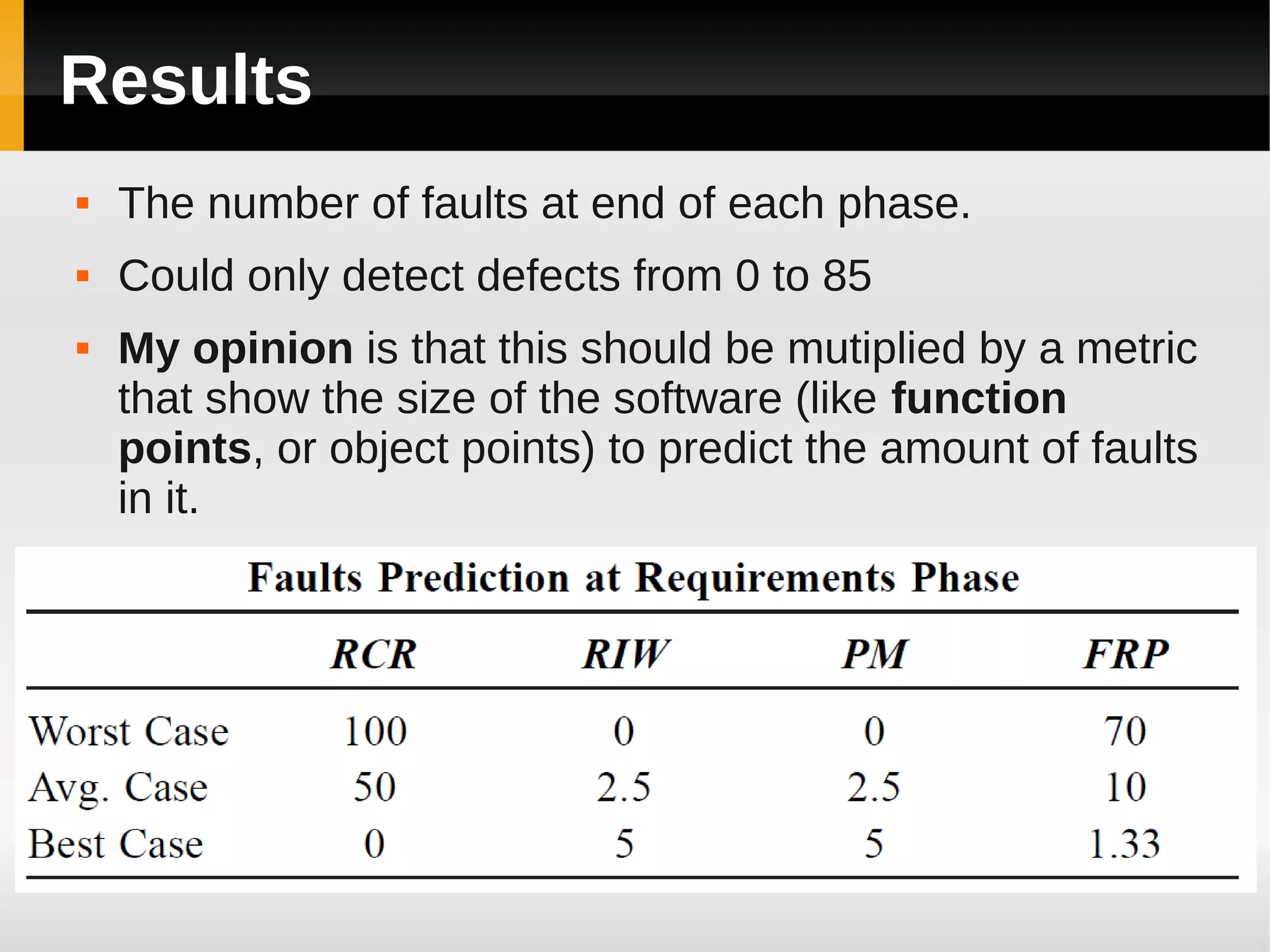
![Results [continued]](https://image.slidesharecdn.com/asurveyoffaultpredictionusingmachinelearningalgorithms-120226104850-phpapp02/75/A-survey-of-fault-prediction-using-machine-learning-algorithms-17-2048.jpg)
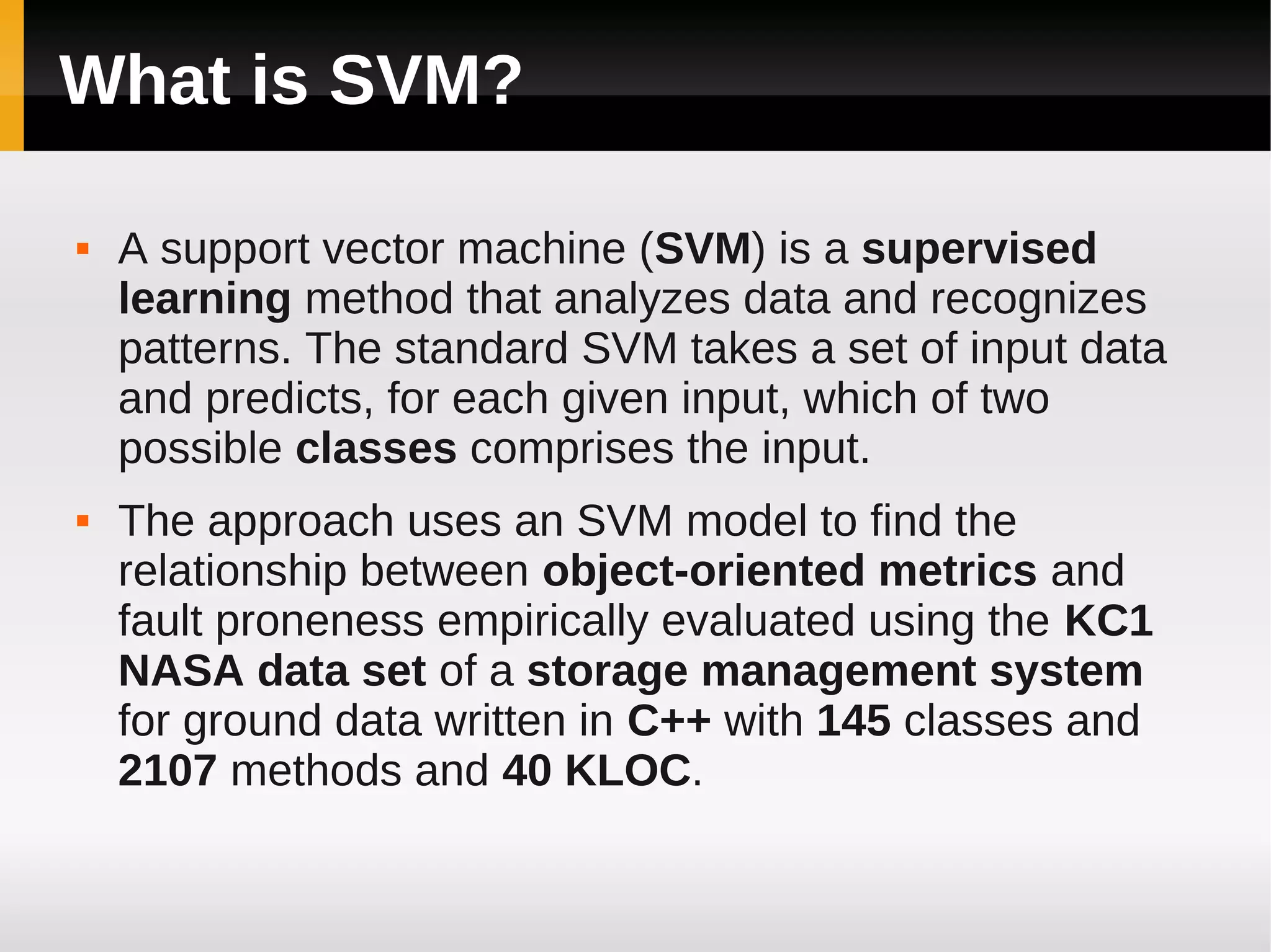
![[2]
Software Fault Proneness
Prediction Using Support
Vector Machines](https://image.slidesharecdn.com/asurveyoffaultpredictionusingmachinelearningalgorithms-120226104850-phpapp02/75/A-survey-of-fault-prediction-using-machine-learning-algorithms-18-2048.jpg)
![Some Measures
Sensitivity is defined as the probability that a module
which contains a fault is correctly classified [7]
Specificity is the proportion of correctly identified fault-
free modules.[7]
Probability of False alarm (PF) is the proportion of
fault-free modules that are classified erroneously.
PF=1-specificity [7]
Precision is the probability of correctly predicting faulty
modules among the modules classified as fault-prone.
[7]
Completeness value, which is defined as the number
of faults in faulty predicted classes divided by the
number of faults in all classes. [8]](https://image.slidesharecdn.com/asurveyoffaultpredictionusingmachinelearningalgorithms-120226104850-phpapp02/75/A-survey-of-fault-prediction-using-machine-learning-algorithms-21-2048.jpg)
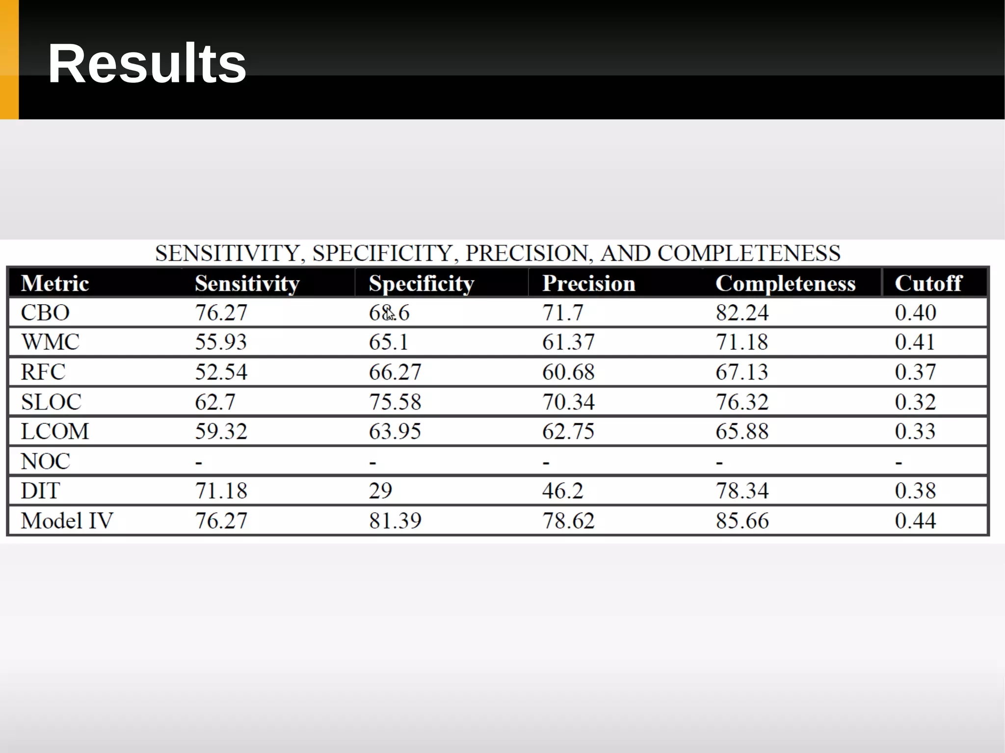
![Results [continued]](https://image.slidesharecdn.com/asurveyoffaultpredictionusingmachinelearningalgorithms-120226104850-phpapp02/75/A-survey-of-fault-prediction-using-machine-learning-algorithms-23-2048.jpg)
![Results [continued]](https://image.slidesharecdn.com/asurveyoffaultpredictionusingmachinelearningalgorithms-120226104850-phpapp02/75/A-survey-of-fault-prediction-using-machine-learning-algorithms-24-2048.jpg)
![Results [continued]
Sensitivity and Completeness of the model](https://image.slidesharecdn.com/asurveyoffaultpredictionusingmachinelearningalgorithms-120226104850-phpapp02/75/A-survey-of-fault-prediction-using-machine-learning-algorithms-25-2048.jpg)
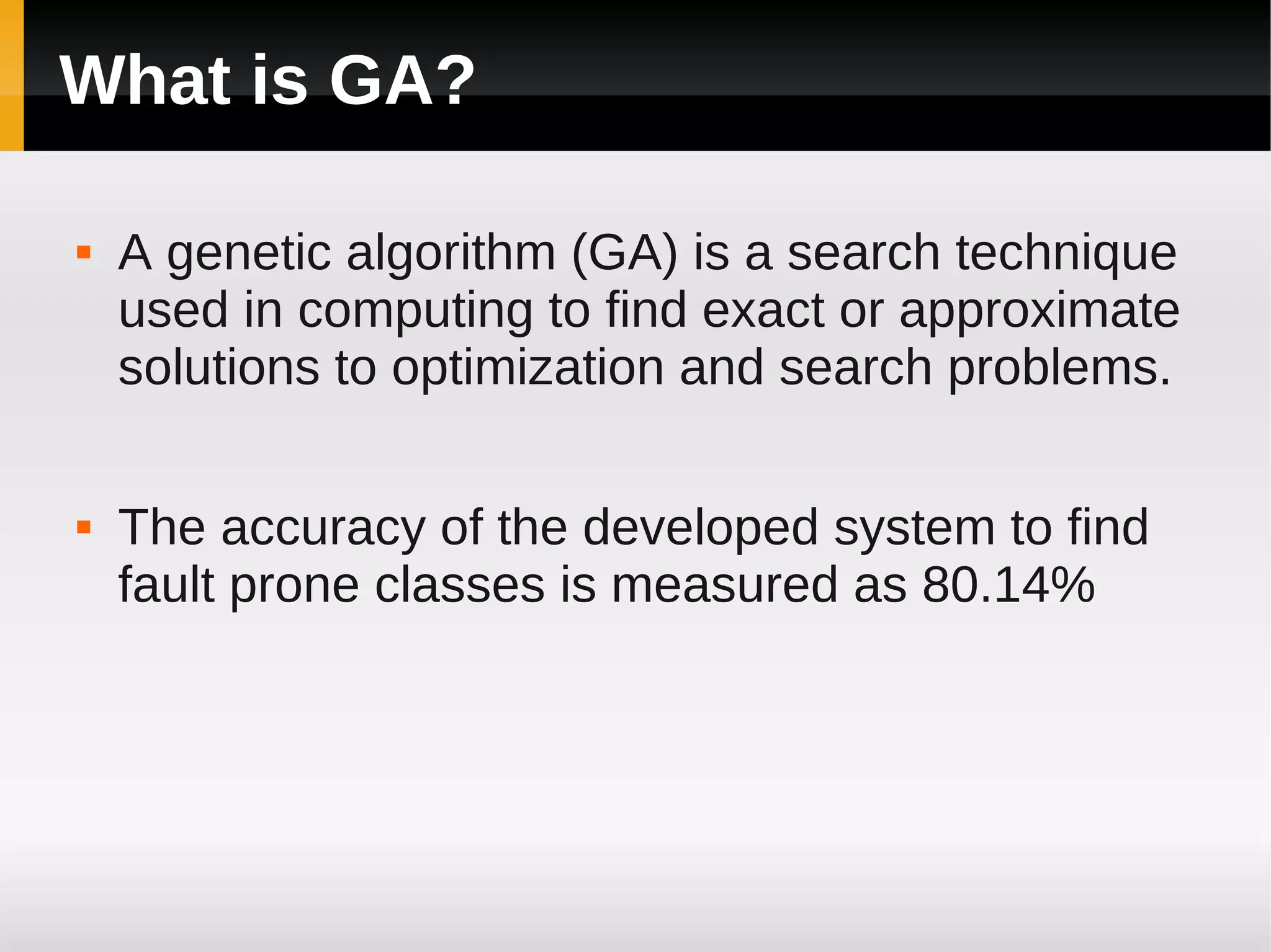
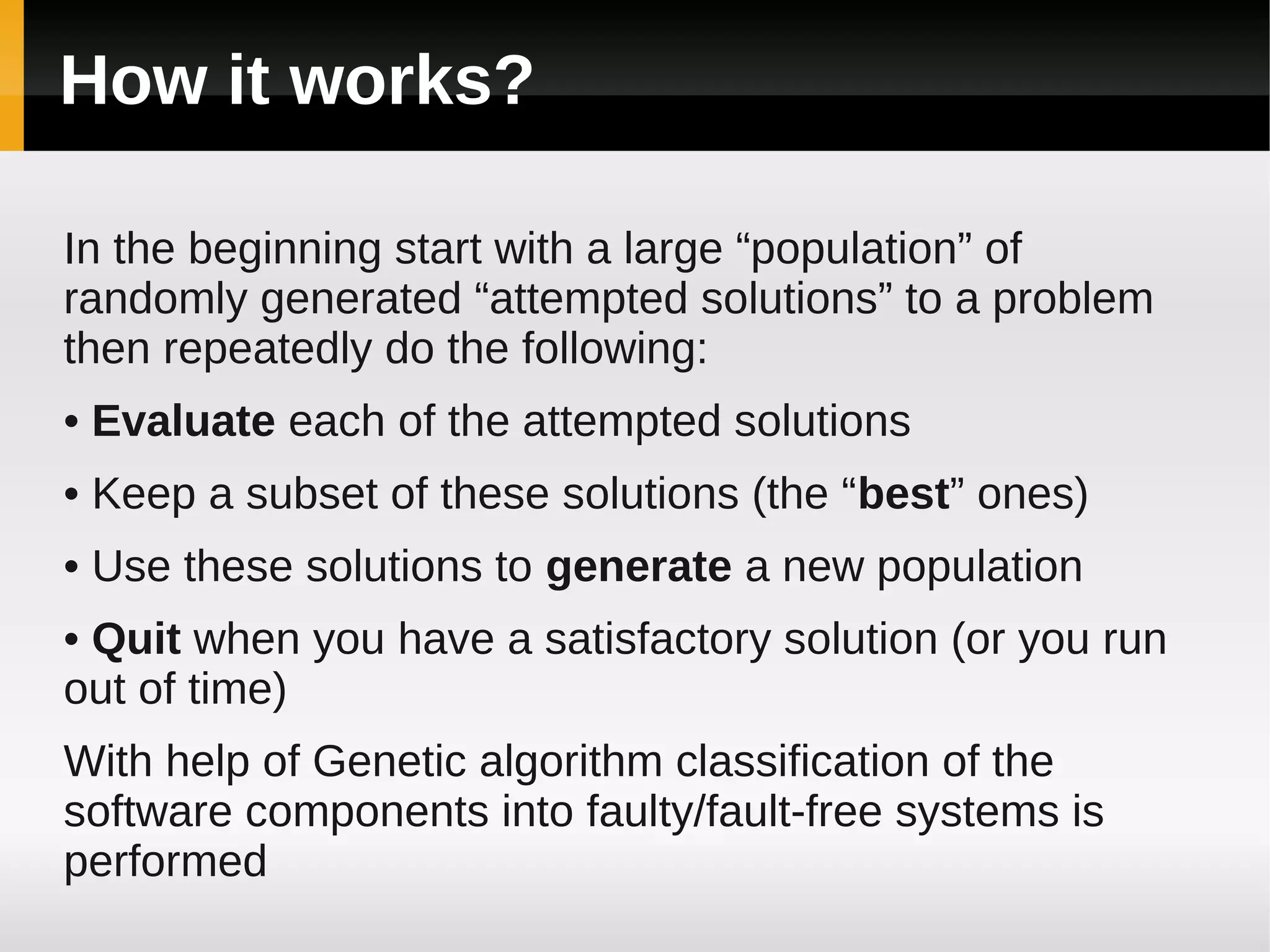
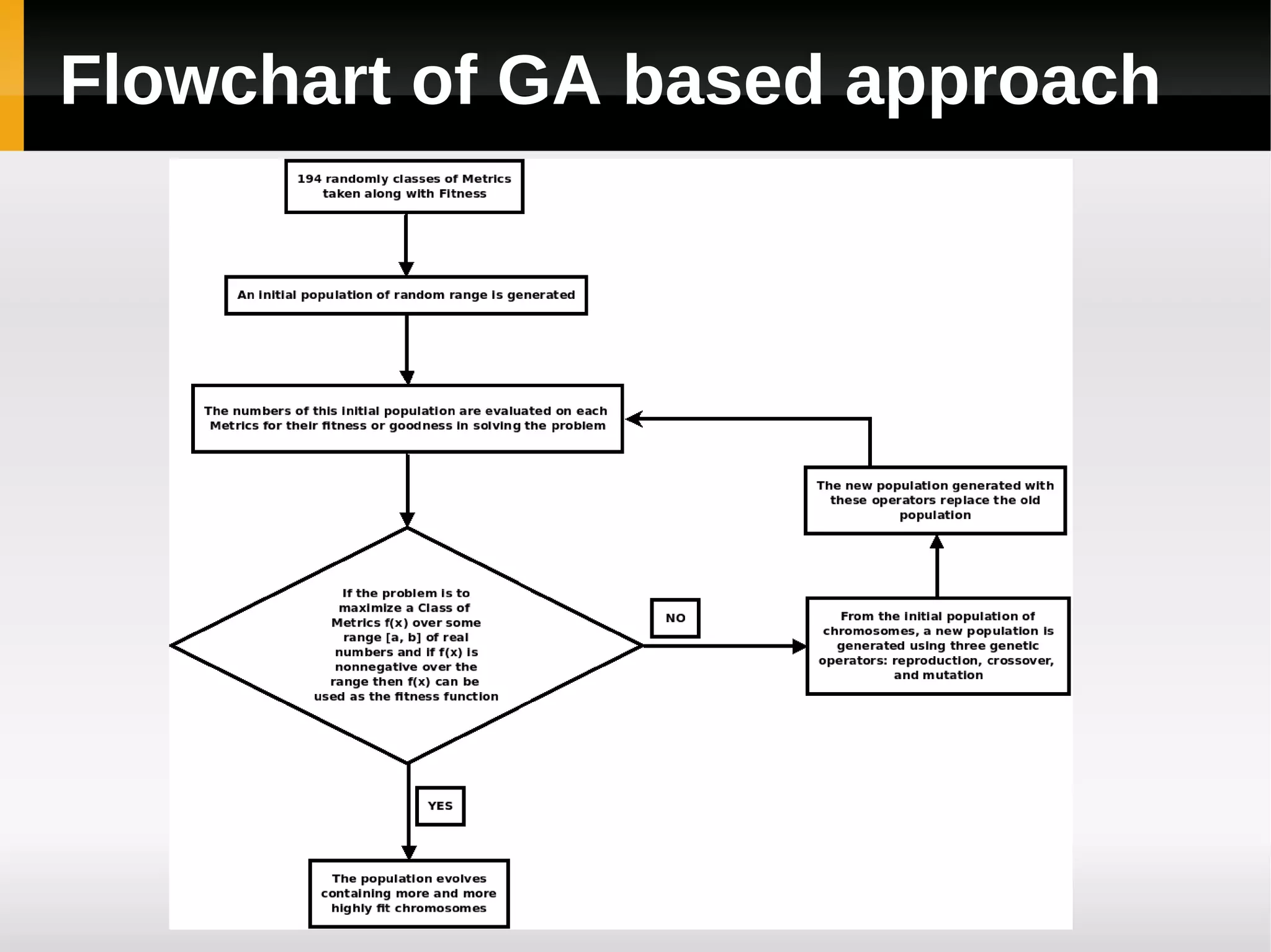
![[3]
A Genetic Algorithm Based
Classification Approach for
Finding Fault Prone Classes](https://image.slidesharecdn.com/asurveyoffaultpredictionusingmachinelearningalgorithms-120226104850-phpapp02/75/A-survey-of-fault-prediction-using-machine-learning-algorithms-26-2048.jpg)
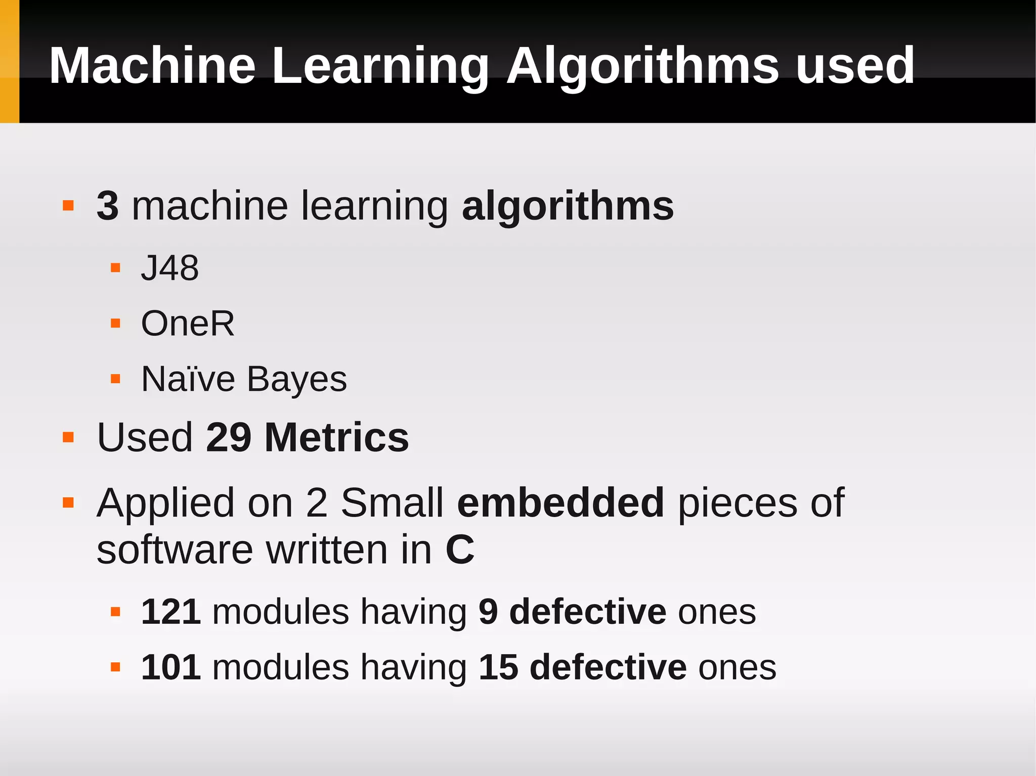
![[4]
Comparing The Effectiveness
Of Machine Learning
Algorithms For Defect
Prediction](https://image.slidesharecdn.com/asurveyoffaultpredictionusingmachinelearningalgorithms-120226104850-phpapp02/75/A-survey-of-fault-prediction-using-machine-learning-algorithms-31-2048.jpg)
![OneR
OneR induces simple rules based on a single
attribute
OneR creates one rule for each attribute in the
training data, then selects the rule with the smallest
error rate to be the only one rule.
Determines the class that appears most often for an
attribute value
A rule is simply a set of attribute values bound to
their majority class.
The error rate is the number of training data instances
that the class of an attribute value does not agree
with the binding for that attribute value in the rule.[4]](https://image.slidesharecdn.com/asurveyoffaultpredictionusingmachinelearningalgorithms-120226104850-phpapp02/75/A-survey-of-fault-prediction-using-machine-learning-algorithms-34-2048.jpg)
![Naïve Bayes
Naïve Bayes: based on theorem of Bayes
posterior probability
Naïve Bayes assumes that all classes are
conditionally independent
i.e. there are no dependence relationship among
the attributes.
Naïve Bayes classifier estimates the
probability of attribute values of each class
from the training set by counting the frequency
of each discrete attribute values. [4]](https://image.slidesharecdn.com/asurveyoffaultpredictionusingmachinelearningalgorithms-120226104850-phpapp02/75/A-survey-of-fault-prediction-using-machine-learning-algorithms-35-2048.jpg)
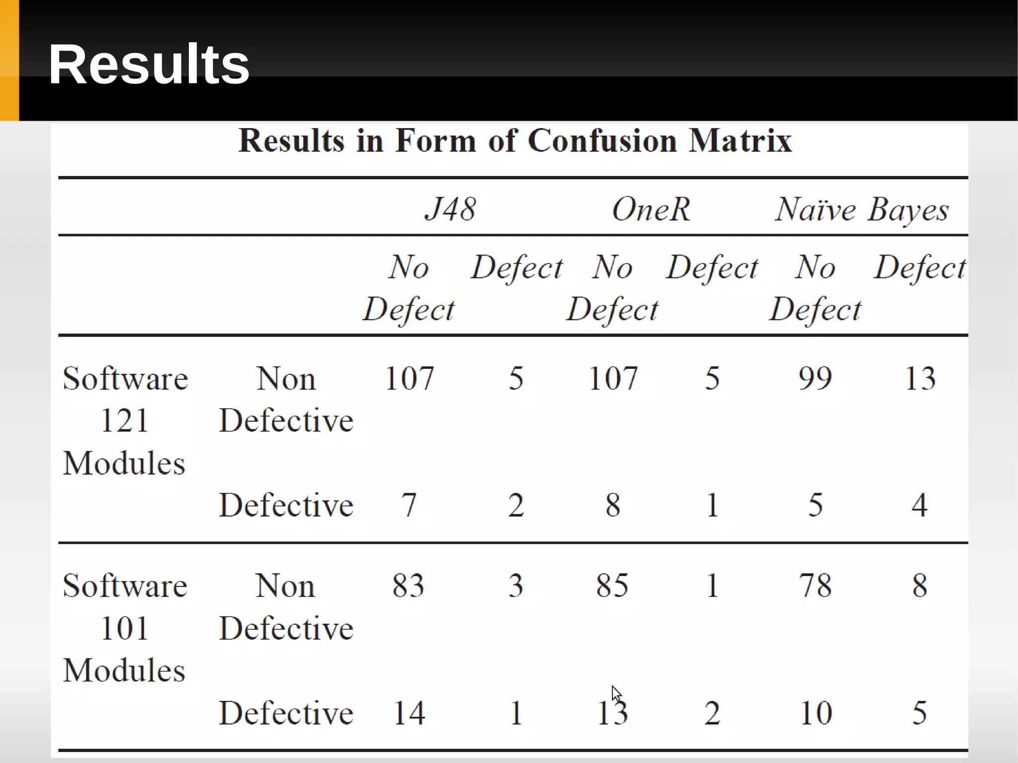
![Results [continued]
J48 and OneR performed better than Naïve
Bayes.
The performance of J48, OneR and Naïve
Bayes for correctly classified instances are
90.086%, 89.2562% and 85.124% respectively.
[4]](https://image.slidesharecdn.com/asurveyoffaultpredictionusingmachinelearningalgorithms-120226104850-phpapp02/75/A-survey-of-fault-prediction-using-machine-learning-algorithms-37-2048.jpg)
![References
[1] A Fuzzy Model for Early Software Fault Prediction
Using Process Maturity and Software Metrics (Ajeet
Kumar Pandey & N. K. Goyal, Reliability Engineering
Centre, IIT Kharagpur, INDIA)
[2] Software Fault Proneness Prediction Using
Support Vector Machines (Yogesh Singh, Arvinder
Kaur, Ruchika Malhotra)
[3] A Genetic Algorithm Based Classification Approach
for Finding Fault Prone Classes (Parvinder S. Sandhu,
Satish Kumar Dhiman, Anmol Goyal)
[4] Comparing The Effectiveness Of Machine Learning
Algorithms For Defect Prediction by Pradeep Singh](https://image.slidesharecdn.com/asurveyoffaultpredictionusingmachinelearningalgorithms-120226104850-phpapp02/75/A-survey-of-fault-prediction-using-machine-learning-algorithms-39-2048.jpg)
![References [continued]
[5] Mining Metrics to Predict Component Failures
(Nachiappan Nagappan, Thomas Ball, and Andreas
Zeller)
[6] Data Mining Static Code Attributes to Learn Defect
Predictors (Tim Menzies, and Jeremy Greenwald)
[7] Techniques for evaluating fault prediction models
(Yue Jiang & Bojan Cukic & Yan Ma)
[8] Empirical Validation of Object-Oriented Metrics on
Open Source Software for Fault Prediction (Tibor
Gyimothy, Rudolf Ferenc, and Istvan Siket)](https://image.slidesharecdn.com/asurveyoffaultpredictionusingmachinelearningalgorithms-120226104850-phpapp02/75/A-survey-of-fault-prediction-using-machine-learning-algorithms-40-2048.jpg)


![Instroduction
The world relies on software heavily now so it
should be reliable
Software Reliability is the probability of a
software system or component to perform its
intended function under the specified
operating conditions over the specified period
of time [1]
In other words the less faults there are in a
software the more reliable it is.](https://crownmelresort.com/image.slidesharecdn.com/asurveyoffaultpredictionusingmachinelearningalgorithms-120226104850-phpapp02/75/A-survey-of-fault-prediction-using-machine-learning-algorithms-2-2048.jpg)

![[1]
A Fuzzy Model for Early Software
Fault Prediction Using Process
Maturity and Software Metrics](https://crownmelresort.com/image.slidesharecdn.com/asurveyoffaultpredictionusingmachinelearningalgorithms-120226104850-phpapp02/75/A-survey-of-fault-prediction-using-machine-learning-algorithms-4-2048.jpg)


![Results [continued]](https://crownmelresort.com/image.slidesharecdn.com/asurveyoffaultpredictionusingmachinelearningalgorithms-120226104850-phpapp02/75/A-survey-of-fault-prediction-using-machine-learning-algorithms-17-2048.jpg)
![[2]
Software Fault Proneness
Prediction Using Support
Vector Machines](https://crownmelresort.com/image.slidesharecdn.com/asurveyoffaultpredictionusingmachinelearningalgorithms-120226104850-phpapp02/75/A-survey-of-fault-prediction-using-machine-learning-algorithms-18-2048.jpg)


![Some Measures
Sensitivity is defined as the probability that a module
which contains a fault is correctly classified [7]
Specificity is the proportion of correctly identified fault-
free modules.[7]
Probability of False alarm (PF) is the proportion of
fault-free modules that are classified erroneously.
PF=1-specificity [7]
Precision is the probability of correctly predicting faulty
modules among the modules classified as fault-prone.
[7]
Completeness value, which is defined as the number
of faults in faulty predicted classes divided by the
number of faults in all classes. [8]](https://crownmelresort.com/image.slidesharecdn.com/asurveyoffaultpredictionusingmachinelearningalgorithms-120226104850-phpapp02/75/A-survey-of-fault-prediction-using-machine-learning-algorithms-21-2048.jpg)

![Results [continued]](https://crownmelresort.com/image.slidesharecdn.com/asurveyoffaultpredictionusingmachinelearningalgorithms-120226104850-phpapp02/75/A-survey-of-fault-prediction-using-machine-learning-algorithms-23-2048.jpg)
![Results [continued]](https://crownmelresort.com/image.slidesharecdn.com/asurveyoffaultpredictionusingmachinelearningalgorithms-120226104850-phpapp02/75/A-survey-of-fault-prediction-using-machine-learning-algorithms-24-2048.jpg)
![Results [continued]
Sensitivity and Completeness of the model](https://crownmelresort.com/image.slidesharecdn.com/asurveyoffaultpredictionusingmachinelearningalgorithms-120226104850-phpapp02/75/A-survey-of-fault-prediction-using-machine-learning-algorithms-25-2048.jpg)
![[3]
A Genetic Algorithm Based
Classification Approach for
Finding Fault Prone Classes](https://crownmelresort.com/image.slidesharecdn.com/asurveyoffaultpredictionusingmachinelearningalgorithms-120226104850-phpapp02/75/A-survey-of-fault-prediction-using-machine-learning-algorithms-26-2048.jpg)


![[4]
Comparing The Effectiveness
Of Machine Learning
Algorithms For Defect
Prediction](https://crownmelresort.com/image.slidesharecdn.com/asurveyoffaultpredictionusingmachinelearningalgorithms-120226104850-phpapp02/75/A-survey-of-fault-prediction-using-machine-learning-algorithms-31-2048.jpg)


![OneR
OneR induces simple rules based on a single
attribute
OneR creates one rule for each attribute in the
training data, then selects the rule with the smallest
error rate to be the only one rule.
Determines the class that appears most often for an
attribute value
A rule is simply a set of attribute values bound to
their majority class.
The error rate is the number of training data instances
that the class of an attribute value does not agree
with the binding for that attribute value in the rule.[4]](https://crownmelresort.com/image.slidesharecdn.com/asurveyoffaultpredictionusingmachinelearningalgorithms-120226104850-phpapp02/75/A-survey-of-fault-prediction-using-machine-learning-algorithms-34-2048.jpg)
![Naïve Bayes
Naïve Bayes: based on theorem of Bayes
posterior probability
Naïve Bayes assumes that all classes are
conditionally independent
i.e. there are no dependence relationship among
the attributes.
Naïve Bayes classifier estimates the
probability of attribute values of each class
from the training set by counting the frequency
of each discrete attribute values. [4]](https://crownmelresort.com/image.slidesharecdn.com/asurveyoffaultpredictionusingmachinelearningalgorithms-120226104850-phpapp02/75/A-survey-of-fault-prediction-using-machine-learning-algorithms-35-2048.jpg)

![Results [continued]
J48 and OneR performed better than Naïve
Bayes.
The performance of J48, OneR and Naïve
Bayes for correctly classified instances are
90.086%, 89.2562% and 85.124% respectively.
[4]](https://crownmelresort.com/image.slidesharecdn.com/asurveyoffaultpredictionusingmachinelearningalgorithms-120226104850-phpapp02/75/A-survey-of-fault-prediction-using-machine-learning-algorithms-37-2048.jpg)

![References
[1] A Fuzzy Model for Early Software Fault Prediction
Using Process Maturity and Software Metrics (Ajeet
Kumar Pandey & N. K. Goyal, Reliability Engineering
Centre, IIT Kharagpur, INDIA)
[2] Software Fault Proneness Prediction Using
Support Vector Machines (Yogesh Singh, Arvinder
Kaur, Ruchika Malhotra)
[3] A Genetic Algorithm Based Classification Approach
for Finding Fault Prone Classes (Parvinder S. Sandhu,
Satish Kumar Dhiman, Anmol Goyal)
[4] Comparing The Effectiveness Of Machine Learning
Algorithms For Defect Prediction by Pradeep Singh](https://crownmelresort.com/image.slidesharecdn.com/asurveyoffaultpredictionusingmachinelearningalgorithms-120226104850-phpapp02/75/A-survey-of-fault-prediction-using-machine-learning-algorithms-39-2048.jpg)
![References [continued]
[5] Mining Metrics to Predict Component Failures
(Nachiappan Nagappan, Thomas Ball, and Andreas
Zeller)
[6] Data Mining Static Code Attributes to Learn Defect
Predictors (Tim Menzies, and Jeremy Greenwald)
[7] Techniques for evaluating fault prediction models
(Yue Jiang & Bojan Cukic & Yan Ma)
[8] Empirical Validation of Object-Oriented Metrics on
Open Source Software for Fault Prediction (Tibor
Gyimothy, Rudolf Ferenc, and Istvan Siket)](https://crownmelresort.com/image.slidesharecdn.com/asurveyoffaultpredictionusingmachinelearningalgorithms-120226104850-phpapp02/75/A-survey-of-fault-prediction-using-machine-learning-algorithms-40-2048.jpg)


The document surveys four machine learning approaches for predicting software faults, emphasizing the importance of software reliability and fault prediction. It discusses methods including fuzzy logic, support vector machines, genetic algorithms, and comparative analysis of machine learning algorithms, highlighting their effectiveness and accuracy in identifying fault-prone software components. The findings suggest that machine learning can significantly aid in early fault prediction, potentially reducing project risks and costs.


![Support, Monitoring, Continuous Improvement & Scaling Agentic Automation [3/3]](https://cdn.slidesharecdn.com/ss_thumbnails/agenticcommunityseries-day3-cfd-251120170304-ddef8112-thumbnail.jpg?width=640&height=640&fit=bounds)