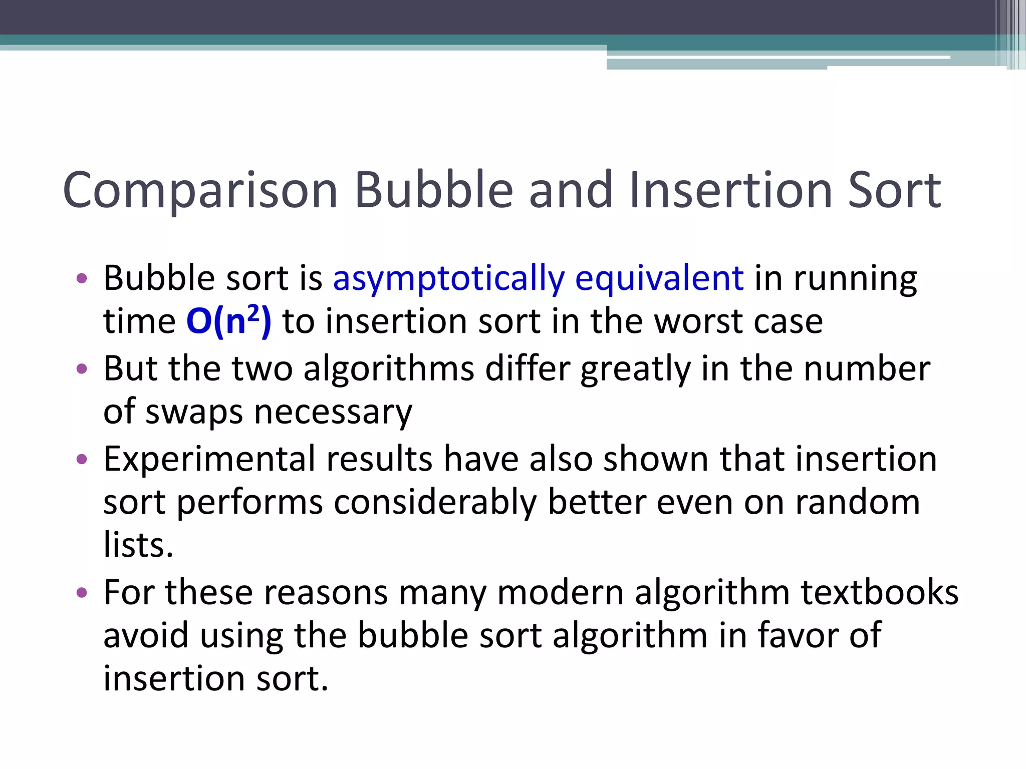
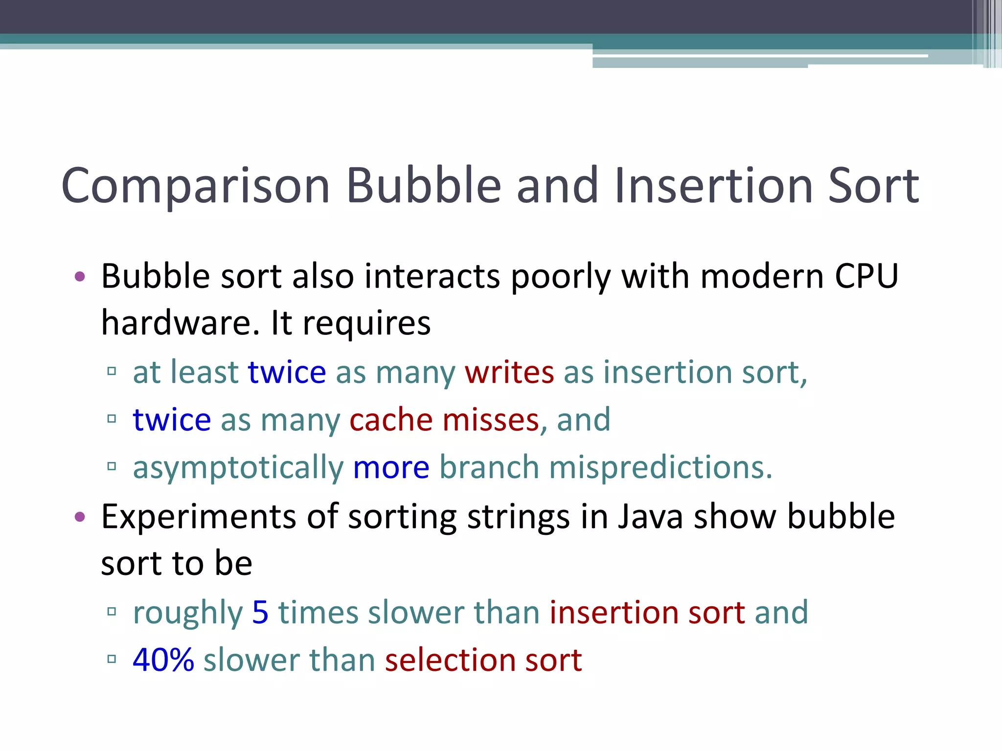
Downloaded 11 times

![Sorting an Array of Integers
• The picture shows an
array of six integers
that we want to sort
from smallest to
largest
0
10
20
30
40
50
60
70
[1] [2] [3] [4] [5] [6][0] [1] [2] [3] [4] [5]](https://image.slidesharecdn.com/week4-sorting-191013065812/75/Sorting-Algorithms-6-2048.jpg)
![0
10
20
30
40
50
60
70
[1] [2] [3] [4] [5] [6]
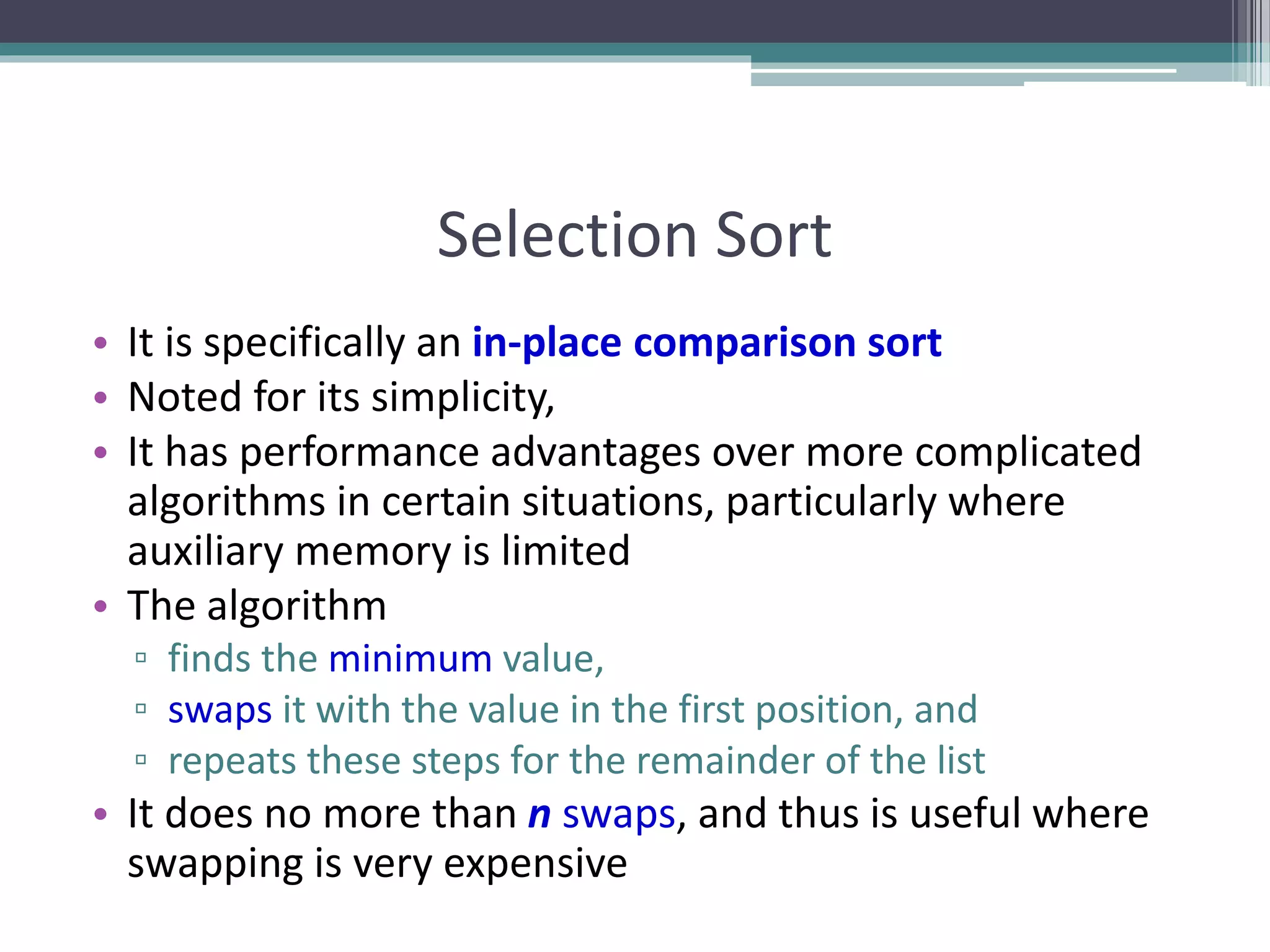
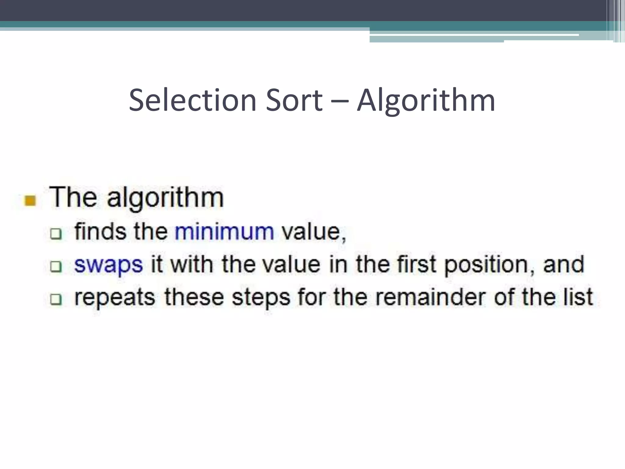
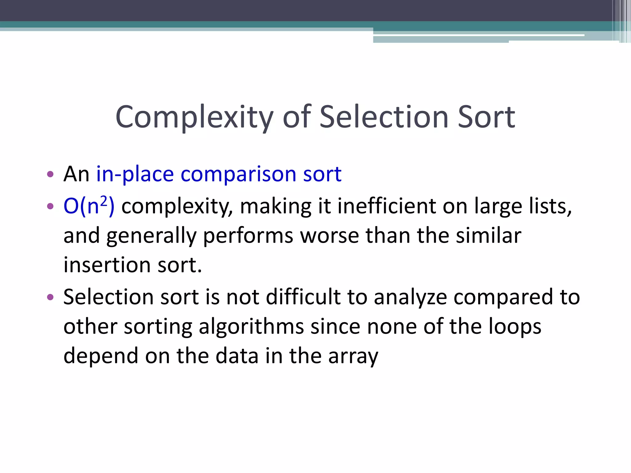
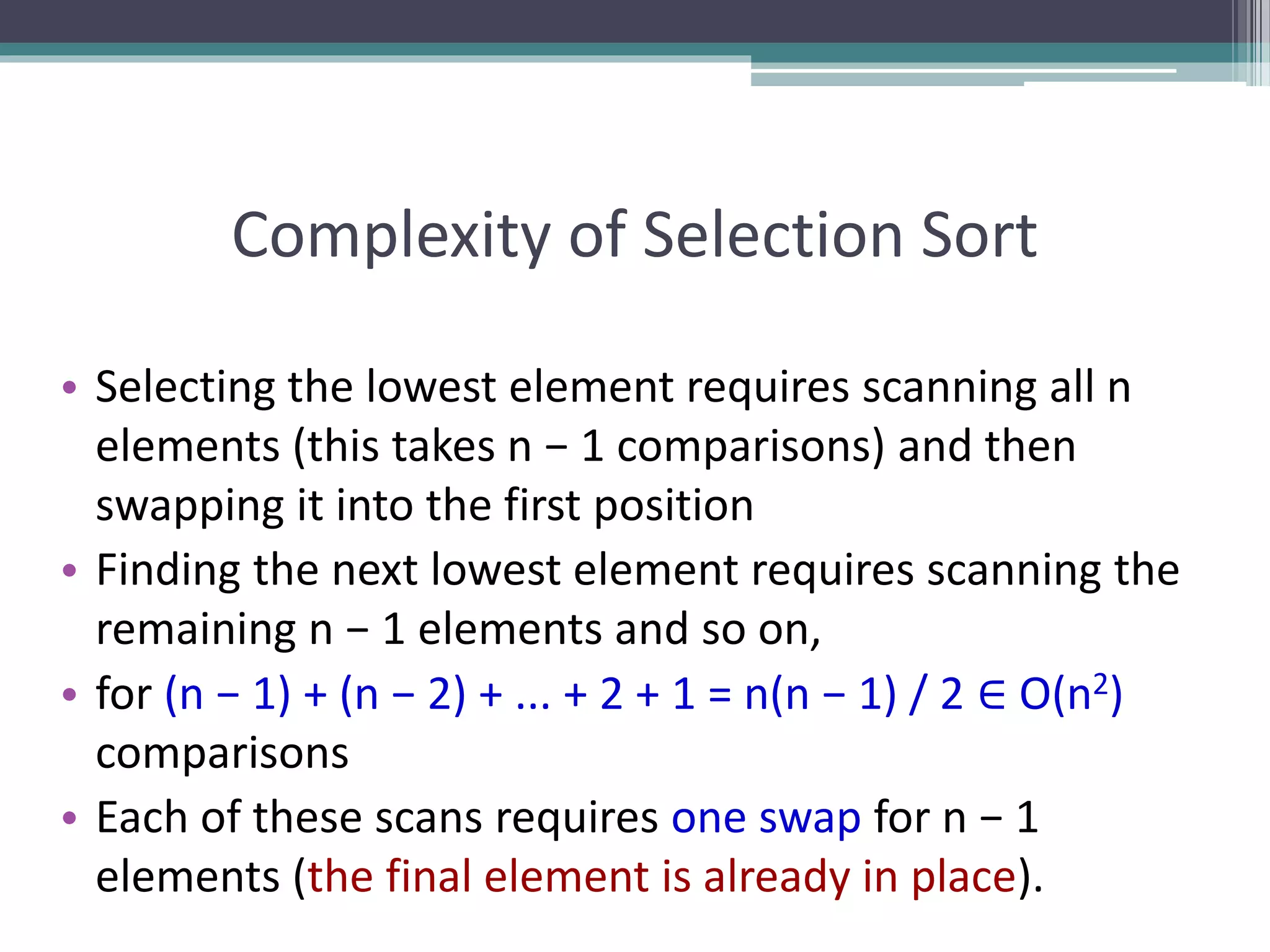
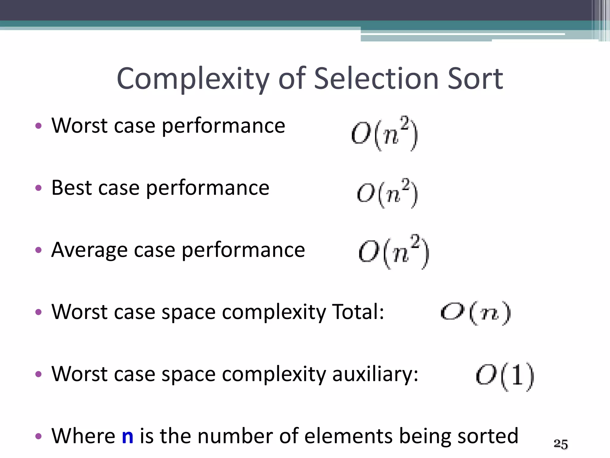
The Selection Sort Algorithm
• Start by finding the
smallest entry.
0
10
20
30
40
50
60
70
[1] [2] [3] [4] [5] [6][0] [1] [2] [3] [4] [5]](https://image.slidesharecdn.com/week4-sorting-191013065812/75/Sorting-Algorithms-7-2048.jpg)
![0
10
20
30
40
50
60
70
[1] [2] [3] [4] [5] [6]
• Start by finding the
smallest entry.
• Swap the smallest
entry with the first
entry.
0
10
20
30
40
50
60
70
[1] [2] [3] [4] [5] [6][0] [1] [2] [3] [4] [5]](https://image.slidesharecdn.com/week4-sorting-191013065812/75/Sorting-Algorithms-8-2048.jpg)
![0
10
20
30
40
50
60
70
[1] [2] [3] [4] [5] [6]
• Start by finding
the smallest
entry.
• Swap the smallest
entry with the
first entry.
0
10
20
30
40
50
60
70
[1] [2] [3] [4] [5] [6][0] [1] [2] [3] [4] [5]](https://image.slidesharecdn.com/week4-sorting-191013065812/75/Sorting-Algorithms-9-2048.jpg)
![0
10
20
30
40
50
60
70
[1] [2] [3] [4] [5] [6]
• Part of the array
is now sorted.
0
10
20
30
40
50
60
70
[1] [2] [3] [4] [5] [6]
Sorted side Unsorted side
[0] [1] [2] [3] [4] [5]](https://image.slidesharecdn.com/week4-sorting-191013065812/75/Sorting-Algorithms-10-2048.jpg)
![0
10
20
30
40
50
60
70
[1] [2] [3] [4] [5] [6]
0
10
20
30
40
50
60
70
[1] [2] [3] [4] [5] [6]
• Find the smallest
element in the
unsorted side.
Sorted side Unsorted side
[0] [1] [2] [3] [4] [5]](https://image.slidesharecdn.com/week4-sorting-191013065812/75/Sorting-Algorithms-11-2048.jpg)
![0
10
20
30
40
50
60
70
[1] [2] [3] [4] [5] [6]
0
10
20
30
40
50
60
70
[1] [2] [3] [4] [5] [6]
• Find the smallest
element in the
unsorted side.
• Swap with the front
of the unsorted
side.
Sorted side Unsorted side
[0] [1] [2] [3] [4] [5]](https://image.slidesharecdn.com/week4-sorting-191013065812/75/Sorting-Algorithms-12-2048.jpg)
![0
10
20
30
40
50
60
70
[1] [2] [3] [4] [5] [6]
0
10
20
30
40
50
60
70
[1] [2] [3] [4] [5] [6]
• We have
increased the size
of the sorted side
by one element.
Sorted side Unsorted side
[0] [1] [2] [3] [4] [5]](https://image.slidesharecdn.com/week4-sorting-191013065812/75/Sorting-Algorithms-13-2048.jpg)
![0
10
20
30
40
50
60
70
[1] [2] [3] [4] [5] [6]
0
10
20
30
40
50
60
70
[1] [2] [3] [4] [5] [6]
• The process
continues...
Sorted side Unsorted side
Smallest
from
unsorted
[0] [1] [2] [3] [4] [5]](https://image.slidesharecdn.com/week4-sorting-191013065812/75/Sorting-Algorithms-14-2048.jpg)
![0
10
20
30
40
50
60
70
[1] [2] [3] [4] [5] [6]
0
10
20
30
40
50
60
70
[1] [2] [3] [4] [5] [6]
• The process
continues...
Sorted side Unsorted side
[0] [1] [2] [3] [4] [5]](https://image.slidesharecdn.com/week4-sorting-191013065812/75/Sorting-Algorithms-15-2048.jpg)
![0
10
20
30
40
50
60
70
[1] [2] [3] [4] [5] [6]
0
10
20
30
40
50
60
70
[1] [2] [3] [4] [5] [6]
• The process
continues...
Sorted side Unsorted side
Sorted side
is bigger
[0] [1] [2] [3] [4] [5]](https://image.slidesharecdn.com/week4-sorting-191013065812/75/Sorting-Algorithms-16-2048.jpg)
![0
10
20
30
40
50
60
70
[1] [2] [3] [4] [5] [6]
0
10
20
30
40
50
60
70
[1] [2] [3] [4] [5] [6]
• The process keeps
adding one more
number to the
sorted side.
• The sorted side has
the smallest
numbers, arranged
from small to large.
Sorted side Unsorted side
[0] [1] [2] [3] [4] [5]](https://image.slidesharecdn.com/week4-sorting-191013065812/75/Sorting-Algorithms-17-2048.jpg)
![0
10
20
30
40
50
60
70
[1] [2] [3] [4] [5] [6]
0
10
20
30
40
50
60
70
[1] [2] [3] [4] [5] [6]
• We can stop when the
unsorted side has just
one number, since
that number must be
the largest number.
[0] [1] [2] [3] [4] [5]
Sorted side Unsorted side](https://image.slidesharecdn.com/week4-sorting-191013065812/75/Sorting-Algorithms-18-2048.jpg)
![0
10
20
30
40
50
60
70
[1] [2] [3] [4] [5] [6]
The Selection Sort Algorithm
• The array is now
sorted.
• We repeatedly
selected the smallest
element, and moved
this element to the
front of the unsorted
side.
[0] [1] [2] [3] [4] [5]](https://image.slidesharecdn.com/week4-sorting-191013065812/75/Sorting-Algorithms-19-2048.jpg)
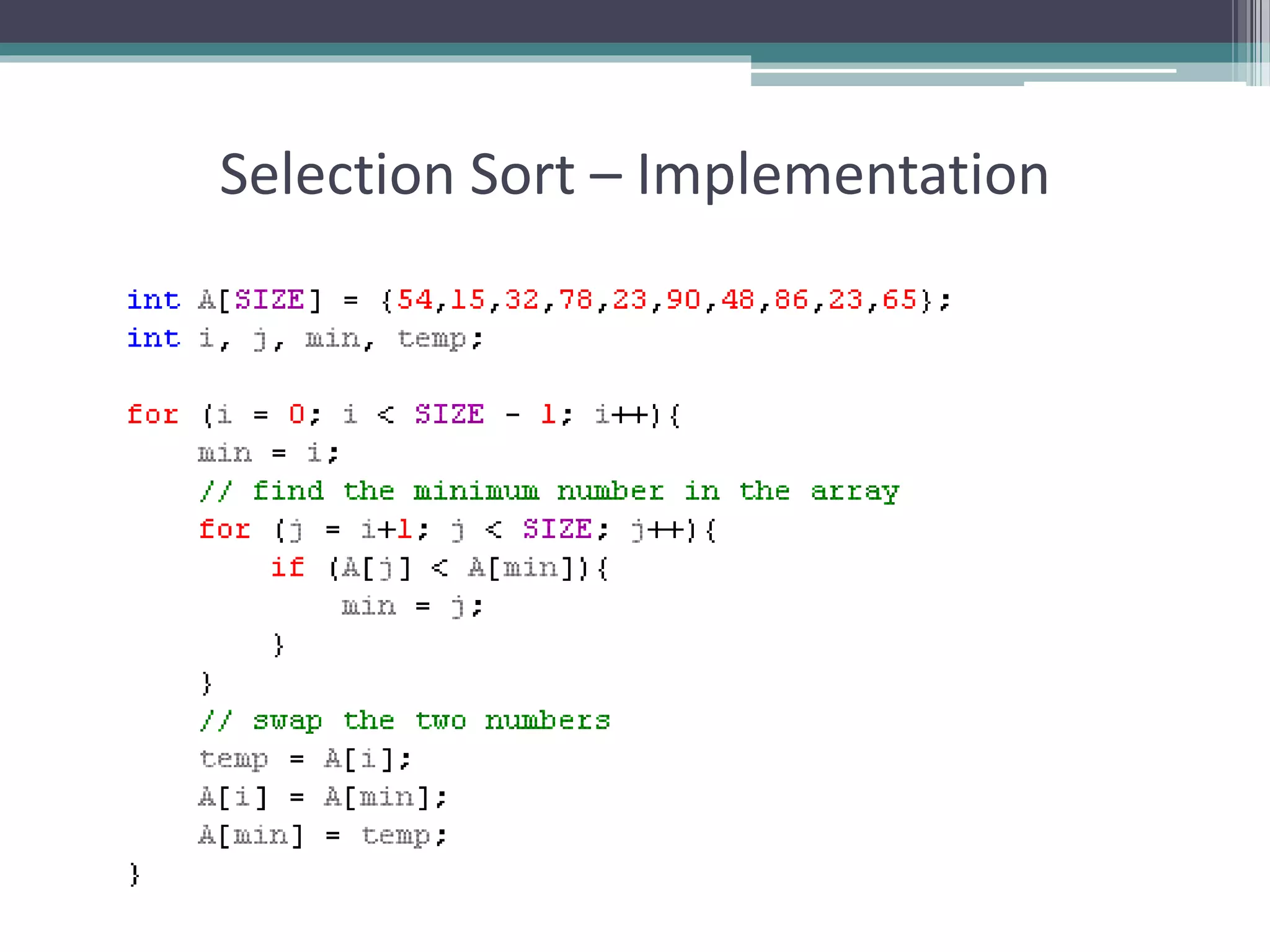
![Selection Sort – Pseudocode
Input: An array A[1..n] of n elements.
Output: A[1..n] sorted in descending order
1. for i 1 to n - 1
2. min i
3. for j i + 1 to n {Find the i th smallest element.}
4. if A[j] < A[min] then
5. min j
6. end for
7. if min i then interchange A[i] and A[min]
8. end for](https://image.slidesharecdn.com/week4-sorting-191013065812/75/Sorting-Algorithms-21-2048.jpg)
![0
10
20
30
40
50
60
70
[1] [2] [3] [4] [5] [6]
The Insertion Sort Algorithm
• Views the array as
having two sides
• a sorted side and
• an unsorted side.
[0] [1] [2] [3] [4] [5]](https://image.slidesharecdn.com/week4-sorting-191013065812/75/Sorting-Algorithms-28-2048.jpg)
![0
10
20
30
40
50
60
70
[1] [2] [3] [4] [5] [6]
• The sorted side
starts with just the
first element, which
is not necessarily
the smallest
element.
0
10
20
30
40
50
60
70
[1] [2] [3] [4] [5] [6][0] [1] [2] [3] [4] [5]
Sorted side Unsorted side](https://image.slidesharecdn.com/week4-sorting-191013065812/75/Sorting-Algorithms-29-2048.jpg)
![0
10
20
30
40
50
60
70
[1] [2] [3] [4] [5] [6]
• The sorted side
grows by taking
the front element
from the
unsorted side...
0
10
20
30
40
50
60
70
[1] [2] [3] [4] [5] [6][0] [1] [2] [3] [4] [5]
Sorted side Unsorted side](https://image.slidesharecdn.com/week4-sorting-191013065812/75/Sorting-Algorithms-30-2048.jpg)
![0
10
20
30
40
50
60
70
[1] [2] [3] [4] [5] [6]
• ...and inserting it
in the place that
keeps the sorted
side arranged
from small to
large.
0
10
20
30
40
50
60
70
[1] [2] [3] [4] [5] [6][0] [1] [2] [3] [4] [5]
Sorted side Unsorted side](https://image.slidesharecdn.com/week4-sorting-191013065812/75/Sorting-Algorithms-31-2048.jpg)
![0
10
20
30
40
50
60
70
[1] [2] [3] [4] [5] [6]
• In this example,
the new element
goes in front of
the element that
was already in the
sorted side.
0
10
20
30
40
50
60
70
[1] [2] [3] [4] [5] [6][0] [1] [2] [3] [4] [5]
Sorted side Unsorted side](https://image.slidesharecdn.com/week4-sorting-191013065812/75/Sorting-Algorithms-32-2048.jpg)
![0
10
20
30
40
50
60
70
[1] [2] [3] [4] [5] [6]
• Sometimes we
are lucky and the
new inserted
item doesn't
need to move at
all.
0
10
20
30
40
50
60
70
[1] [2] [3] [4] [5] [6][0] [1] [2] [3] [4] [5]
Sorted side Unsorted side](https://image.slidesharecdn.com/week4-sorting-191013065812/75/Sorting-Algorithms-33-2048.jpg)
![0
10
20
30
40
50
60
70
[1] [2] [3] [4] [5] [6]
• Sometimes we
are lucky twice in
a row.
0
10
20
30
40
50
60
70
[1] [2] [3] [4] [5] [6][0] [1] [2] [3] [4] [5]
Sorted side Unsorted side](https://image.slidesharecdn.com/week4-sorting-191013065812/75/Sorting-Algorithms-34-2048.jpg)
![0
10
20
30
40
50
60
70
[1] [2] [3] [4] [5] [6]
Copy the new
element to a
separate location.
0
10
20
30
40
50
60
70
[1] [2] [3] [4] [5] [6]
3] [4] [5] [6]
[0] [1] [2] [3] [4] [5]
Sorted side Unsorted side](https://image.slidesharecdn.com/week4-sorting-191013065812/75/Sorting-Algorithms-35-2048.jpg)
![0
10
20
30
40
50
60
70
[1] [2] [3] [4] [5] [6]
Shift elements in
the sorted side,
creating an open
space for the new
element.
0
10
20
30
40
50
60
70
[1] [2] [3] [4] [5] [6]
3] [4] [5] [6]
[0] [1] [2] [3] [4] [5]](https://image.slidesharecdn.com/week4-sorting-191013065812/75/Sorting-Algorithms-36-2048.jpg)
![0
10
20
30
40
50
60
70
[1] [2] [3] [4] [5] [6]
0
10
20
30
40
50
60
70
[1] [2] [3] [4] [5] [6]
Shift elements in
the sorted side,
creating an open
space for the new
element.
3] [4] [5] [6]
0
10
20
30
40
50
60
70
[1] [2] [3] [4] [5] [6][0] [1] [2] [3] [4] [5]](https://image.slidesharecdn.com/week4-sorting-191013065812/75/Sorting-Algorithms-37-2048.jpg)
![0
10
20
30
40
50
60
70
[1] [2] [3] [4] [5] [6]
0
10
20
30
40
50
60
70
[1] [2] [3] [4] [5] [6]
Continue shifting
elements...
3] [4] [5] [6]
0
10
20
30
40
50
60
70
[1] [2] [3] [4] [5] [6][0] [1] [2] [3] [4] [5]](https://image.slidesharecdn.com/week4-sorting-191013065812/75/Sorting-Algorithms-38-2048.jpg)
![0
10
20
30
40
50
60
70
[1] [2] [3] [4] [5] [6]
0
10
20
30
40
50
60
70
[1] [2] [3] [4] [5] [6]
Continue shifting
elements...
3] [4] [5] [6]
0
10
20
30
40
50
60
70
[1] [2] [3] [4] [5] [6][0] [1] [2] [3] [4] [5]](https://image.slidesharecdn.com/week4-sorting-191013065812/75/Sorting-Algorithms-39-2048.jpg)
![0
10
20
30
40
50
60
70
[1] [2] [3] [4] [5] [6]
0
10
20
30
40
50
60
70
[1] [2] [3] [4] [5] [6]
...until you reach
the location for
the new element.
3] [4] [5] [6]
0
10
20
30
40
50
60
70
[1] [2] [3] [4] [5] [6][0] [1] [2] [3] [4] [5]](https://image.slidesharecdn.com/week4-sorting-191013065812/75/Sorting-Algorithms-40-2048.jpg)
![0
10
20
30
40
50
60
70
[1] [2] [3] [4] [5] [6]
0
10
20
30
40
50
60
70
[1] [2] [3] [4] [5] [6]
Copy the new
element back into
the array, at the
correct location.
3] [4] [5] [6]
[0] [1] [2] [3] [4] [5]
Sorted side Unsorted side](https://image.slidesharecdn.com/week4-sorting-191013065812/75/Sorting-Algorithms-41-2048.jpg)
![0
10
20
30
40
50
60
70
[1] [2] [3] [4] [5] [6]
3] [4] [5] [6]
• The last element
must also be
inserted. Start by
copying it...
[0] [1] [2] [3] [4] [5]
Sorted side Unsorted side](https://image.slidesharecdn.com/week4-sorting-191013065812/75/Sorting-Algorithms-42-2048.jpg)
![0
10
20
30
40
50
60
70
[1] [2] [3] [4] [5] [6]
0
10
20
30
40
50
60
70
[1] [2] [3] [4] [5] [6]
How many shifts
will occur before
we copy this
element back into
the array?
3] [4] [5] [6]
[0] [1] [2] [3] [4] [5]](https://image.slidesharecdn.com/week4-sorting-191013065812/75/Sorting-Algorithms-43-2048.jpg)
![0
10
20
30
40
50
60
70
[1] [2] [3] [4] [5] [6]
0
10
20
30
40
50
60
70
[1] [2] [3] [4] [5] [6]
3] [4] [5] [6]
• Four items are
shifted.
[0] [1] [2] [3] [4] [5]](https://image.slidesharecdn.com/week4-sorting-191013065812/75/Sorting-Algorithms-44-2048.jpg)
![0
10
20
30
40
50
60
70
[1] [2] [3] [4] [5] [6]
3] [4] [5] [6]
• Four items are
shifted.
•And then the
element is copied
back into the array.
[0] [1] [2] [3] [4] [5]
The Insertion Sort Algorithm](https://image.slidesharecdn.com/week4-sorting-191013065812/75/Sorting-Algorithms-45-2048.jpg)
![Insertion Sort - Algorithm
For i = 2 to n do the following
a. set NextElement = x[i] and
x[0] = nextElement
b. set j = i
c. While nextElement < x[j – 1] do following
set x[j] equal to x[j – 1]
decrement j by 1
End wile
d. set x[j] equal to nextElement
End for](https://image.slidesharecdn.com/week4-sorting-191013065812/75/Sorting-Algorithms-47-2048.jpg)
![Insertion Sort - Pseudocode
Input: An array A[1..n] of n elements.
Output: A[1..n] sorted in nondecreasing order.
1. for i 2 to n
2. x A[i]
3. j i - 1
4. while (j >0) and (A[j] > x)
5. A[j + 1] A[j]
6. j j - 1
7. end while
8. A[j + 1] x
9. end for](https://image.slidesharecdn.com/week4-sorting-191013065812/75/Sorting-Algorithms-48-2048.jpg)
![Insertion Sort - Implementation
void InsertionSort(int list[], int size){
int i,j,k,temp;
for(i=1;i < size;i++) {
temp=list[i];
j=i;
while((j > 0)&&(temp < list[j-1]) {
list[j]=list[j-1];
j--;
} // end while
list[j]=temp;
} // end for loop
} // end function](https://image.slidesharecdn.com/week4-sorting-191013065812/75/Sorting-Algorithms-49-2048.jpg)
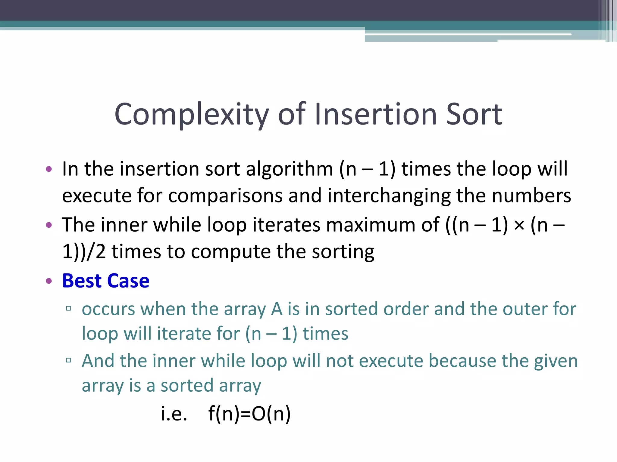
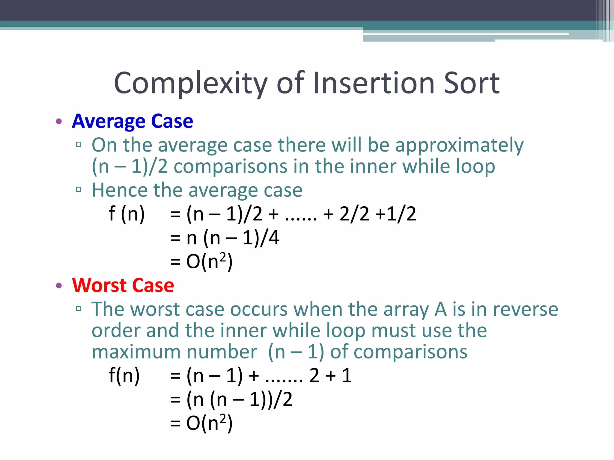
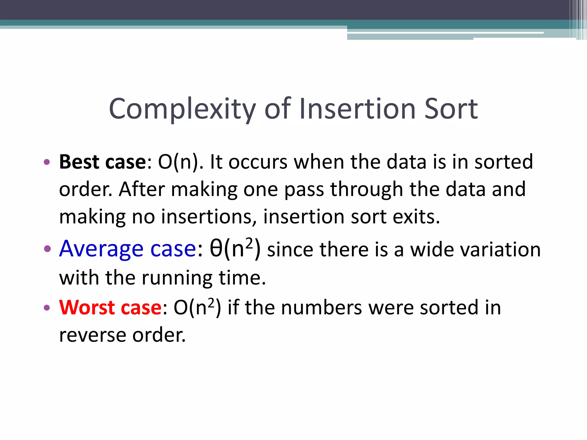
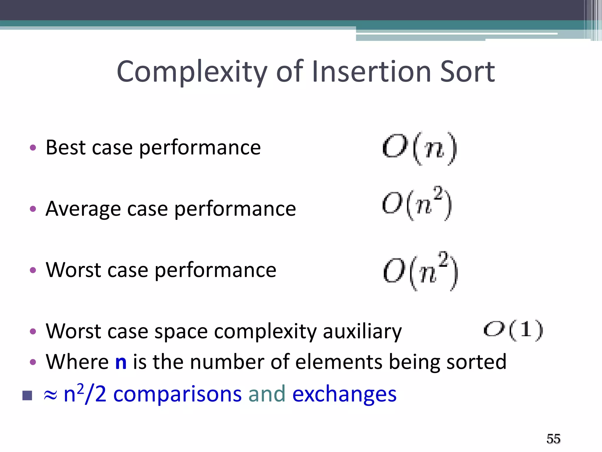
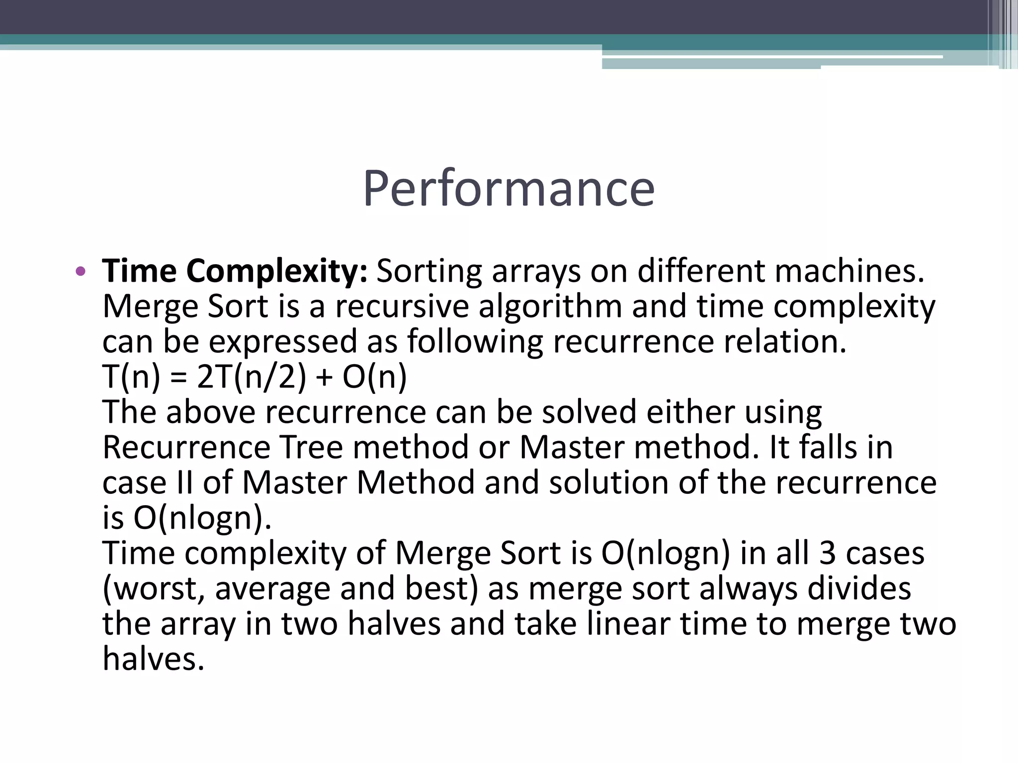
![Complexity of Insertion Sort
The minimum # of element comparisons (best case) occurs when
the array is already sorted in nondecreasing order. In this case,
the # of element comparisons is exactly n - 1, as each element
A[i], 2 ≤ i ≤ n, is compared with A[i - 1] only.
The maximum # of element comparisons (Worst case) occurs if the
array is already sorted in decreasing order and all elements are
distinct. In this case, the number is
n n-1
∑ (i – 1) = ∑ (i – 1) = n(n-1)/2
i =2 i =1
This is because each element A[i], 2 ≤ i ≤ n is
compared with each entry in subarray A[1 .. i-1]
Pros: Relatively simple and easy to implement.
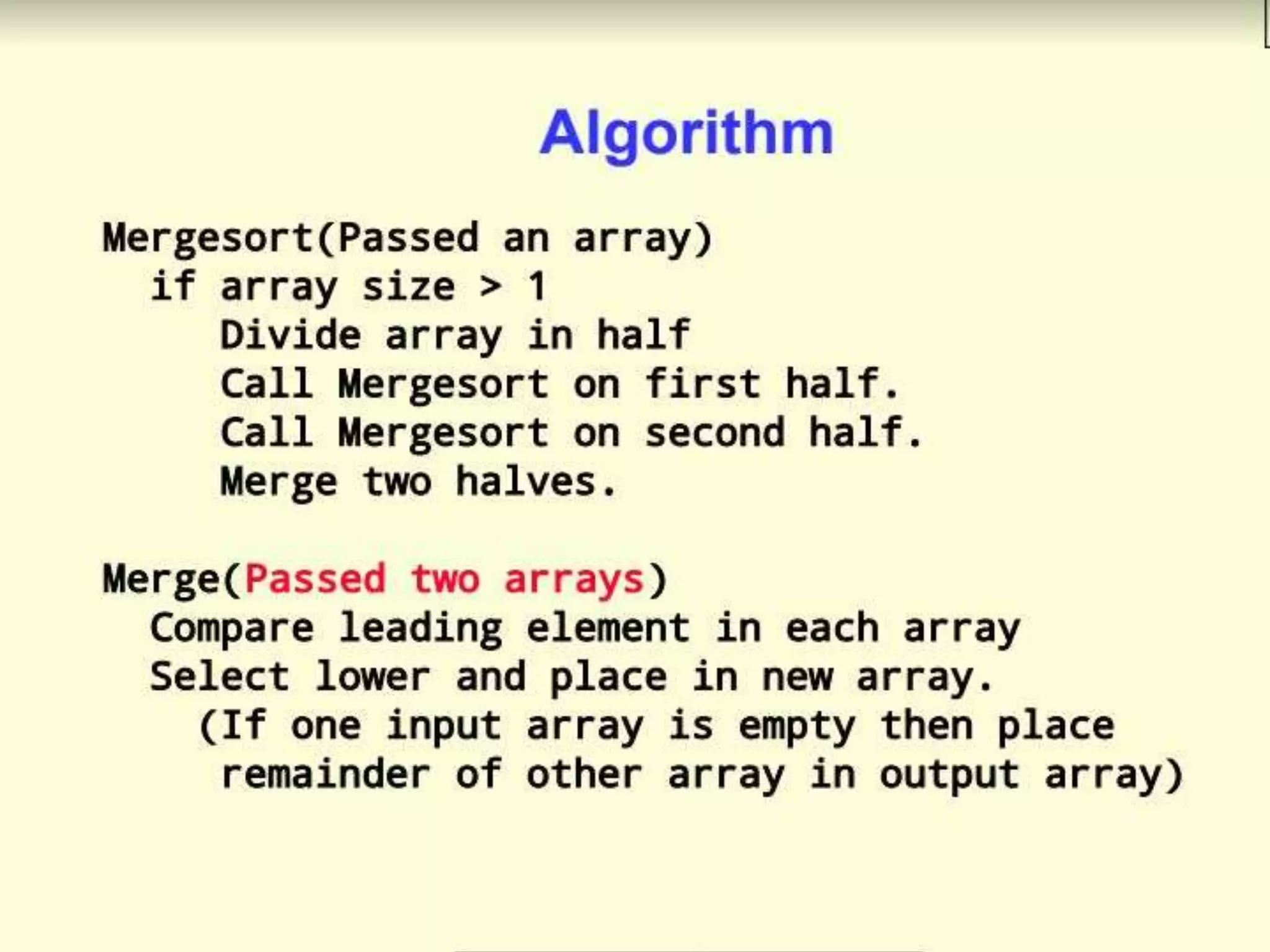
Cons: Inefficient for large lists.](https://image.slidesharecdn.com/week4-sorting-191013065812/75/Sorting-Algorithms-51-2048.jpg)
![Merge Sort
• Like QuickSort, Merge Sort is a Divide and Conquer
algorithm. It divides input array in two halves, calls
itself for the two halves and then merges the two
sorted halves. The merge() function is used for
merging two halves. The merge(arr, l, m, r) is key
process that assumes that arr[l..m] and arr[m+1..r]
are sorted and merges the two sorted sub-arrays into
one.](https://image.slidesharecdn.com/week4-sorting-191013065812/75/Sorting-Algorithms-60-2048.jpg)
![Merge Sort - Implementation
• void MergeSort(int LIST[], int lo, int hi)
• {
• int mid;
• if(lo < hi)
• {
• mid = (lo + hi)/ 2;
• MergeSort(LIST, lo, mid);
• MergeSort(LIST, mid+1, hi);
• ListMerger(LIST, lo, mid, hi);
• }
• }
• void ListMerger(int List[], int lo, int mid, int hi)
• {
• int TempList[hi-lo+1];
//temporary merger array
• int i = lo, j = mid + 1; //i is for left-hand,j is for right-hand
• int k = 0;
//k is for the temporary array
• while(i <= mid && j <=hi)
• {
• if(List[i] <= List[j])
• TempList[k++] = List[i++];
• else
• TempList[k++] = List[j++];
• }](https://image.slidesharecdn.com/week4-sorting-191013065812/75/Sorting-Algorithms-63-2048.jpg)
![Merge Sort - Implementation
• //remaining elements of left-half
• while(i <= mid)
• TempList[k++] = List[i++];
• //remaining elements of right-half
• while(j <= hi)
• TempList[k++] = List[j++];
• //copy the mergered temporary List to the original List
• for(k = 0, i = lo; i <= hi; ++i, ++k)
• List[i] = TempList[k];
•
• }](https://image.slidesharecdn.com/week4-sorting-191013065812/75/Sorting-Algorithms-64-2048.jpg)


![Sorting an Array of Integers
• The picture shows an
array of six integers
that we want to sort
from smallest to
largest
0
10
20
30
40
50
60
70
[1] [2] [3] [4] [5] [6][0] [1] [2] [3] [4] [5]](https://crownmelresort.com/image.slidesharecdn.com/week4-sorting-191013065812/75/Sorting-Algorithms-6-2048.jpg)
![0
10
20
30
40
50
60
70
[1] [2] [3] [4] [5] [6]
The Selection Sort Algorithm
• Start by finding the
smallest entry.
0
10
20
30
40
50
60
70
[1] [2] [3] [4] [5] [6][0] [1] [2] [3] [4] [5]](https://crownmelresort.com/image.slidesharecdn.com/week4-sorting-191013065812/75/Sorting-Algorithms-7-2048.jpg)
![0
10
20
30
40
50
60
70
[1] [2] [3] [4] [5] [6]
• Start by finding the
smallest entry.
• Swap the smallest
entry with the first
entry.
0
10
20
30
40
50
60
70
[1] [2] [3] [4] [5] [6][0] [1] [2] [3] [4] [5]](https://crownmelresort.com/image.slidesharecdn.com/week4-sorting-191013065812/75/Sorting-Algorithms-8-2048.jpg)
![0
10
20
30
40
50
60
70
[1] [2] [3] [4] [5] [6]
• Start by finding
the smallest
entry.
• Swap the smallest
entry with the
first entry.
0
10
20
30
40
50
60
70
[1] [2] [3] [4] [5] [6][0] [1] [2] [3] [4] [5]](https://crownmelresort.com/image.slidesharecdn.com/week4-sorting-191013065812/75/Sorting-Algorithms-9-2048.jpg)
![0
10
20
30
40
50
60
70
[1] [2] [3] [4] [5] [6]
• Part of the array
is now sorted.
0
10
20
30
40
50
60
70
[1] [2] [3] [4] [5] [6]
Sorted side Unsorted side
[0] [1] [2] [3] [4] [5]](https://crownmelresort.com/image.slidesharecdn.com/week4-sorting-191013065812/75/Sorting-Algorithms-10-2048.jpg)
![0
10
20
30
40
50
60
70
[1] [2] [3] [4] [5] [6]
0
10
20
30
40
50
60
70
[1] [2] [3] [4] [5] [6]
• Find the smallest
element in the
unsorted side.
Sorted side Unsorted side
[0] [1] [2] [3] [4] [5]](https://crownmelresort.com/image.slidesharecdn.com/week4-sorting-191013065812/75/Sorting-Algorithms-11-2048.jpg)
![0
10
20
30
40
50
60
70
[1] [2] [3] [4] [5] [6]
0
10
20
30
40
50
60
70
[1] [2] [3] [4] [5] [6]
• Find the smallest
element in the
unsorted side.
• Swap with the front
of the unsorted
side.
Sorted side Unsorted side
[0] [1] [2] [3] [4] [5]](https://crownmelresort.com/image.slidesharecdn.com/week4-sorting-191013065812/75/Sorting-Algorithms-12-2048.jpg)
![0
10
20
30
40
50
60
70
[1] [2] [3] [4] [5] [6]
0
10
20
30
40
50
60
70
[1] [2] [3] [4] [5] [6]
• We have
increased the size
of the sorted side
by one element.
Sorted side Unsorted side
[0] [1] [2] [3] [4] [5]](https://crownmelresort.com/image.slidesharecdn.com/week4-sorting-191013065812/75/Sorting-Algorithms-13-2048.jpg)
![0
10
20
30
40
50
60
70
[1] [2] [3] [4] [5] [6]
0
10
20
30
40
50
60
70
[1] [2] [3] [4] [5] [6]
• The process
continues...
Sorted side Unsorted side
Smallest
from
unsorted
[0] [1] [2] [3] [4] [5]](https://crownmelresort.com/image.slidesharecdn.com/week4-sorting-191013065812/75/Sorting-Algorithms-14-2048.jpg)
![0
10
20
30
40
50
60
70
[1] [2] [3] [4] [5] [6]
0
10
20
30
40
50
60
70
[1] [2] [3] [4] [5] [6]
• The process
continues...
Sorted side Unsorted side
[0] [1] [2] [3] [4] [5]](https://crownmelresort.com/image.slidesharecdn.com/week4-sorting-191013065812/75/Sorting-Algorithms-15-2048.jpg)
![0
10
20
30
40
50
60
70
[1] [2] [3] [4] [5] [6]
0
10
20
30
40
50
60
70
[1] [2] [3] [4] [5] [6]
• The process
continues...
Sorted side Unsorted side
Sorted side
is bigger
[0] [1] [2] [3] [4] [5]](https://crownmelresort.com/image.slidesharecdn.com/week4-sorting-191013065812/75/Sorting-Algorithms-16-2048.jpg)
![0
10
20
30
40
50
60
70
[1] [2] [3] [4] [5] [6]
0
10
20
30
40
50
60
70
[1] [2] [3] [4] [5] [6]
• The process keeps
adding one more
number to the
sorted side.
• The sorted side has
the smallest
numbers, arranged
from small to large.
Sorted side Unsorted side
[0] [1] [2] [3] [4] [5]](https://crownmelresort.com/image.slidesharecdn.com/week4-sorting-191013065812/75/Sorting-Algorithms-17-2048.jpg)
![0
10
20
30
40
50
60
70
[1] [2] [3] [4] [5] [6]
0
10
20
30
40
50
60
70
[1] [2] [3] [4] [5] [6]
• We can stop when the
unsorted side has just
one number, since
that number must be
the largest number.
[0] [1] [2] [3] [4] [5]
Sorted side Unsorted side](https://crownmelresort.com/image.slidesharecdn.com/week4-sorting-191013065812/75/Sorting-Algorithms-18-2048.jpg)
![0
10
20
30
40
50
60
70
[1] [2] [3] [4] [5] [6]
The Selection Sort Algorithm
• The array is now
sorted.
• We repeatedly
selected the smallest
element, and moved
this element to the
front of the unsorted
side.
[0] [1] [2] [3] [4] [5]](https://crownmelresort.com/image.slidesharecdn.com/week4-sorting-191013065812/75/Sorting-Algorithms-19-2048.jpg)

![Selection Sort – Pseudocode
Input: An array A[1..n] of n elements.
Output: A[1..n] sorted in descending order
1. for i 1 to n - 1
2. min i
3. for j i + 1 to n {Find the i th smallest element.}
4. if A[j] < A[min] then
5. min j
6. end for
7. if min i then interchange A[i] and A[min]
8. end for](https://crownmelresort.com/image.slidesharecdn.com/week4-sorting-191013065812/75/Sorting-Algorithms-21-2048.jpg)


![0
10
20
30
40
50
60
70
[1] [2] [3] [4] [5] [6]
The Insertion Sort Algorithm
• Views the array as
having two sides
• a sorted side and
• an unsorted side.
[0] [1] [2] [3] [4] [5]](https://crownmelresort.com/image.slidesharecdn.com/week4-sorting-191013065812/75/Sorting-Algorithms-28-2048.jpg)
![0
10
20
30
40
50
60
70
[1] [2] [3] [4] [5] [6]
• The sorted side
starts with just the
first element, which
is not necessarily
the smallest
element.
0
10
20
30
40
50
60
70
[1] [2] [3] [4] [5] [6][0] [1] [2] [3] [4] [5]
Sorted side Unsorted side](https://crownmelresort.com/image.slidesharecdn.com/week4-sorting-191013065812/75/Sorting-Algorithms-29-2048.jpg)
![0
10
20
30
40
50
60
70
[1] [2] [3] [4] [5] [6]
• The sorted side
grows by taking
the front element
from the
unsorted side...
0
10
20
30
40
50
60
70
[1] [2] [3] [4] [5] [6][0] [1] [2] [3] [4] [5]
Sorted side Unsorted side](https://crownmelresort.com/image.slidesharecdn.com/week4-sorting-191013065812/75/Sorting-Algorithms-30-2048.jpg)
![0
10
20
30
40
50
60
70
[1] [2] [3] [4] [5] [6]
• ...and inserting it
in the place that
keeps the sorted
side arranged
from small to
large.
0
10
20
30
40
50
60
70
[1] [2] [3] [4] [5] [6][0] [1] [2] [3] [4] [5]
Sorted side Unsorted side](https://crownmelresort.com/image.slidesharecdn.com/week4-sorting-191013065812/75/Sorting-Algorithms-31-2048.jpg)
![0
10
20
30
40
50
60
70
[1] [2] [3] [4] [5] [6]
• In this example,
the new element
goes in front of
the element that
was already in the
sorted side.
0
10
20
30
40
50
60
70
[1] [2] [3] [4] [5] [6][0] [1] [2] [3] [4] [5]
Sorted side Unsorted side](https://crownmelresort.com/image.slidesharecdn.com/week4-sorting-191013065812/75/Sorting-Algorithms-32-2048.jpg)
![0
10
20
30
40
50
60
70
[1] [2] [3] [4] [5] [6]
• Sometimes we
are lucky and the
new inserted
item doesn't
need to move at
all.
0
10
20
30
40
50
60
70
[1] [2] [3] [4] [5] [6][0] [1] [2] [3] [4] [5]
Sorted side Unsorted side](https://crownmelresort.com/image.slidesharecdn.com/week4-sorting-191013065812/75/Sorting-Algorithms-33-2048.jpg)
![0
10
20
30
40
50
60
70
[1] [2] [3] [4] [5] [6]
• Sometimes we
are lucky twice in
a row.
0
10
20
30
40
50
60
70
[1] [2] [3] [4] [5] [6][0] [1] [2] [3] [4] [5]
Sorted side Unsorted side](https://crownmelresort.com/image.slidesharecdn.com/week4-sorting-191013065812/75/Sorting-Algorithms-34-2048.jpg)
![0
10
20
30
40
50
60
70
[1] [2] [3] [4] [5] [6]
Copy the new
element to a
separate location.
0
10
20
30
40
50
60
70
[1] [2] [3] [4] [5] [6]
3] [4] [5] [6]
[0] [1] [2] [3] [4] [5]
Sorted side Unsorted side](https://crownmelresort.com/image.slidesharecdn.com/week4-sorting-191013065812/75/Sorting-Algorithms-35-2048.jpg)
![0
10
20
30
40
50
60
70
[1] [2] [3] [4] [5] [6]
Shift elements in
the sorted side,
creating an open
space for the new
element.
0
10
20
30
40
50
60
70
[1] [2] [3] [4] [5] [6]
3] [4] [5] [6]
[0] [1] [2] [3] [4] [5]](https://crownmelresort.com/image.slidesharecdn.com/week4-sorting-191013065812/75/Sorting-Algorithms-36-2048.jpg)
![0
10
20
30
40
50
60
70
[1] [2] [3] [4] [5] [6]
0
10
20
30
40
50
60
70
[1] [2] [3] [4] [5] [6]
Shift elements in
the sorted side,
creating an open
space for the new
element.
3] [4] [5] [6]
0
10
20
30
40
50
60
70
[1] [2] [3] [4] [5] [6][0] [1] [2] [3] [4] [5]](https://crownmelresort.com/image.slidesharecdn.com/week4-sorting-191013065812/75/Sorting-Algorithms-37-2048.jpg)
![0
10
20
30
40
50
60
70
[1] [2] [3] [4] [5] [6]
0
10
20
30
40
50
60
70
[1] [2] [3] [4] [5] [6]
Continue shifting
elements...
3] [4] [5] [6]
0
10
20
30
40
50
60
70
[1] [2] [3] [4] [5] [6][0] [1] [2] [3] [4] [5]](https://crownmelresort.com/image.slidesharecdn.com/week4-sorting-191013065812/75/Sorting-Algorithms-38-2048.jpg)
![0
10
20
30
40
50
60
70
[1] [2] [3] [4] [5] [6]
0
10
20
30
40
50
60
70
[1] [2] [3] [4] [5] [6]
Continue shifting
elements...
3] [4] [5] [6]
0
10
20
30
40
50
60
70
[1] [2] [3] [4] [5] [6][0] [1] [2] [3] [4] [5]](https://crownmelresort.com/image.slidesharecdn.com/week4-sorting-191013065812/75/Sorting-Algorithms-39-2048.jpg)
![0
10
20
30
40
50
60
70
[1] [2] [3] [4] [5] [6]
0
10
20
30
40
50
60
70
[1] [2] [3] [4] [5] [6]
...until you reach
the location for
the new element.
3] [4] [5] [6]
0
10
20
30
40
50
60
70
[1] [2] [3] [4] [5] [6][0] [1] [2] [3] [4] [5]](https://crownmelresort.com/image.slidesharecdn.com/week4-sorting-191013065812/75/Sorting-Algorithms-40-2048.jpg)
![0
10
20
30
40
50
60
70
[1] [2] [3] [4] [5] [6]
0
10
20
30
40
50
60
70
[1] [2] [3] [4] [5] [6]
Copy the new
element back into
the array, at the
correct location.
3] [4] [5] [6]
[0] [1] [2] [3] [4] [5]
Sorted side Unsorted side](https://crownmelresort.com/image.slidesharecdn.com/week4-sorting-191013065812/75/Sorting-Algorithms-41-2048.jpg)
![0
10
20
30
40
50
60
70
[1] [2] [3] [4] [5] [6]
3] [4] [5] [6]
• The last element
must also be
inserted. Start by
copying it...
[0] [1] [2] [3] [4] [5]
Sorted side Unsorted side](https://crownmelresort.com/image.slidesharecdn.com/week4-sorting-191013065812/75/Sorting-Algorithms-42-2048.jpg)
![0
10
20
30
40
50
60
70
[1] [2] [3] [4] [5] [6]
0
10
20
30
40
50
60
70
[1] [2] [3] [4] [5] [6]
How many shifts
will occur before
we copy this
element back into
the array?
3] [4] [5] [6]
[0] [1] [2] [3] [4] [5]](https://crownmelresort.com/image.slidesharecdn.com/week4-sorting-191013065812/75/Sorting-Algorithms-43-2048.jpg)
![0
10
20
30
40
50
60
70
[1] [2] [3] [4] [5] [6]
0
10
20
30
40
50
60
70
[1] [2] [3] [4] [5] [6]
3] [4] [5] [6]
• Four items are
shifted.
[0] [1] [2] [3] [4] [5]](https://crownmelresort.com/image.slidesharecdn.com/week4-sorting-191013065812/75/Sorting-Algorithms-44-2048.jpg)
![0
10
20
30
40
50
60
70
[1] [2] [3] [4] [5] [6]
3] [4] [5] [6]
• Four items are
shifted.
•And then the
element is copied
back into the array.
[0] [1] [2] [3] [4] [5]
The Insertion Sort Algorithm](https://crownmelresort.com/image.slidesharecdn.com/week4-sorting-191013065812/75/Sorting-Algorithms-45-2048.jpg)

![Insertion Sort - Algorithm
For i = 2 to n do the following
a. set NextElement = x[i] and
x[0] = nextElement
b. set j = i
c. While nextElement < x[j – 1] do following
set x[j] equal to x[j – 1]
decrement j by 1
End wile
d. set x[j] equal to nextElement
End for](https://crownmelresort.com/image.slidesharecdn.com/week4-sorting-191013065812/75/Sorting-Algorithms-47-2048.jpg)
![Insertion Sort - Pseudocode
Input: An array A[1..n] of n elements.
Output: A[1..n] sorted in nondecreasing order.
1. for i 2 to n
2. x A[i]
3. j i - 1
4. while (j >0) and (A[j] > x)
5. A[j + 1] A[j]
6. j j - 1
7. end while
8. A[j + 1] x
9. end for](https://crownmelresort.com/image.slidesharecdn.com/week4-sorting-191013065812/75/Sorting-Algorithms-48-2048.jpg)
![Insertion Sort - Implementation
void InsertionSort(int list[], int size){
int i,j,k,temp;
for(i=1;i < size;i++) {
temp=list[i];
j=i;
while((j > 0)&&(temp < list[j-1]) {
list[j]=list[j-1];
j--;
} // end while
list[j]=temp;
} // end for loop
} // end function](https://crownmelresort.com/image.slidesharecdn.com/week4-sorting-191013065812/75/Sorting-Algorithms-49-2048.jpg)

![Complexity of Insertion Sort
The minimum # of element comparisons (best case) occurs when
the array is already sorted in nondecreasing order. In this case,
the # of element comparisons is exactly n - 1, as each element
A[i], 2 ≤ i ≤ n, is compared with A[i - 1] only.
The maximum # of element comparisons (Worst case) occurs if the
array is already sorted in decreasing order and all elements are
distinct. In this case, the number is
n n-1
∑ (i – 1) = ∑ (i – 1) = n(n-1)/2
i =2 i =1
This is because each element A[i], 2 ≤ i ≤ n is
compared with each entry in subarray A[1 .. i-1]
Pros: Relatively simple and easy to implement.
Cons: Inefficient for large lists.](https://crownmelresort.com/image.slidesharecdn.com/week4-sorting-191013065812/75/Sorting-Algorithms-51-2048.jpg)


![Merge Sort
• Like QuickSort, Merge Sort is a Divide and Conquer
algorithm. It divides input array in two halves, calls
itself for the two halves and then merges the two
sorted halves. The merge() function is used for
merging two halves. The merge(arr, l, m, r) is key
process that assumes that arr[l..m] and arr[m+1..r]
are sorted and merges the two sorted sub-arrays into
one.](https://crownmelresort.com/image.slidesharecdn.com/week4-sorting-191013065812/75/Sorting-Algorithms-60-2048.jpg)


![Merge Sort - Implementation
• void MergeSort(int LIST[], int lo, int hi)
• {
• int mid;
• if(lo < hi)
• {
• mid = (lo + hi)/ 2;
• MergeSort(LIST, lo, mid);
• MergeSort(LIST, mid+1, hi);
• ListMerger(LIST, lo, mid, hi);
• }
• }
• void ListMerger(int List[], int lo, int mid, int hi)
• {
• int TempList[hi-lo+1];
//temporary merger array
• int i = lo, j = mid + 1; //i is for left-hand,j is for right-hand
• int k = 0;
//k is for the temporary array
• while(i <= mid && j <=hi)
• {
• if(List[i] <= List[j])
• TempList[k++] = List[i++];
• else
• TempList[k++] = List[j++];
• }](https://crownmelresort.com/image.slidesharecdn.com/week4-sorting-191013065812/75/Sorting-Algorithms-63-2048.jpg)
![Merge Sort - Implementation
• //remaining elements of left-half
• while(i <= mid)
• TempList[k++] = List[i++];
• //remaining elements of right-half
• while(j <= hi)
• TempList[k++] = List[j++];
• //copy the mergered temporary List to the original List
• for(k = 0, i = lo; i <= hi; ++i, ++k)
• List[i] = TempList[k];
•
• }](https://crownmelresort.com/image.slidesharecdn.com/week4-sorting-191013065812/75/Sorting-Algorithms-64-2048.jpg)


The document summarizes several sorting algorithms, focusing on selection sort and insertion sort. Selection sort efficiently finds the smallest element and places it at the front, while insertion sort builds a sorted array by inserting elements from an unsorted section. Both algorithms are analyzed in terms of their time complexity and implementation details.