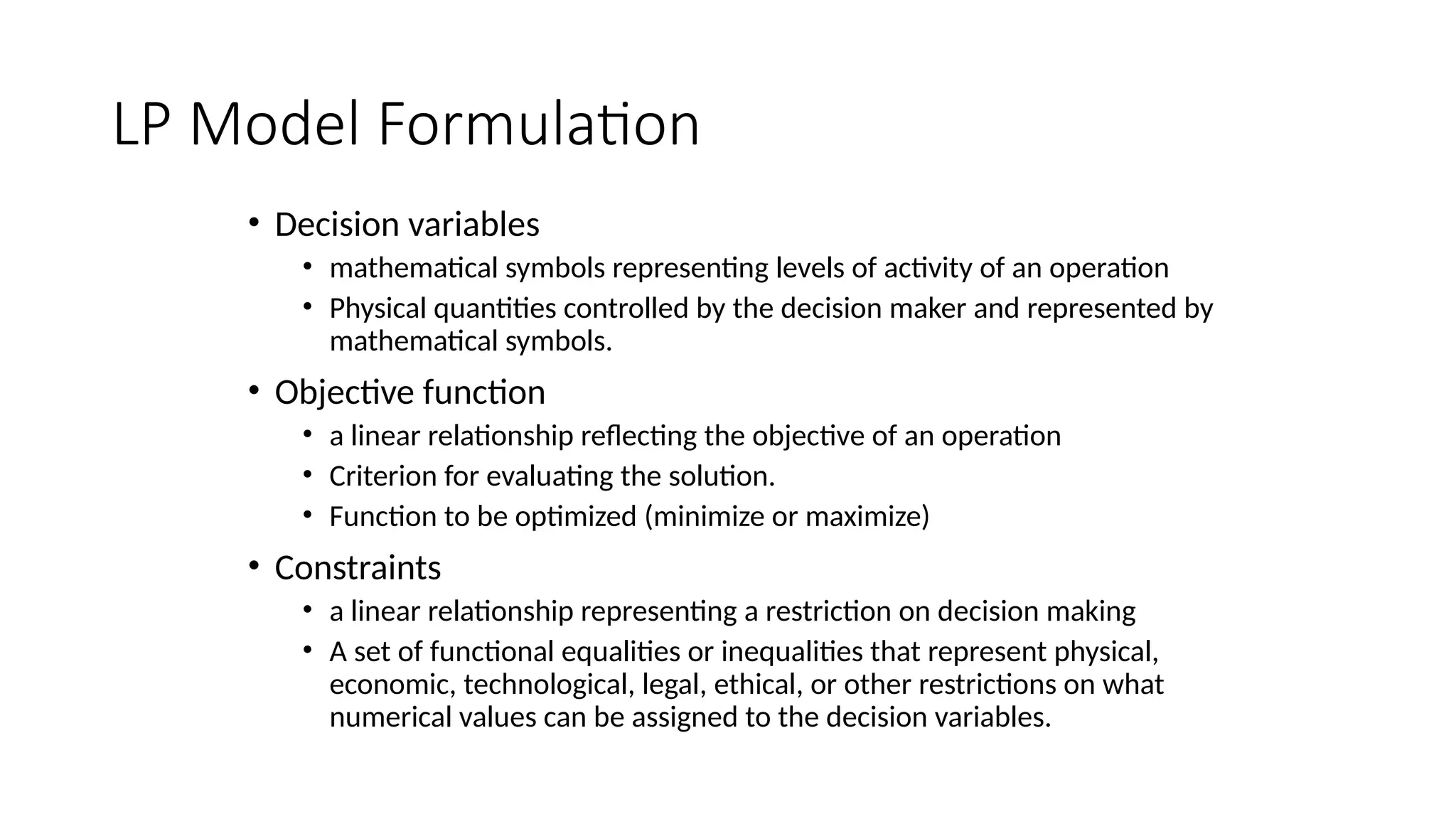
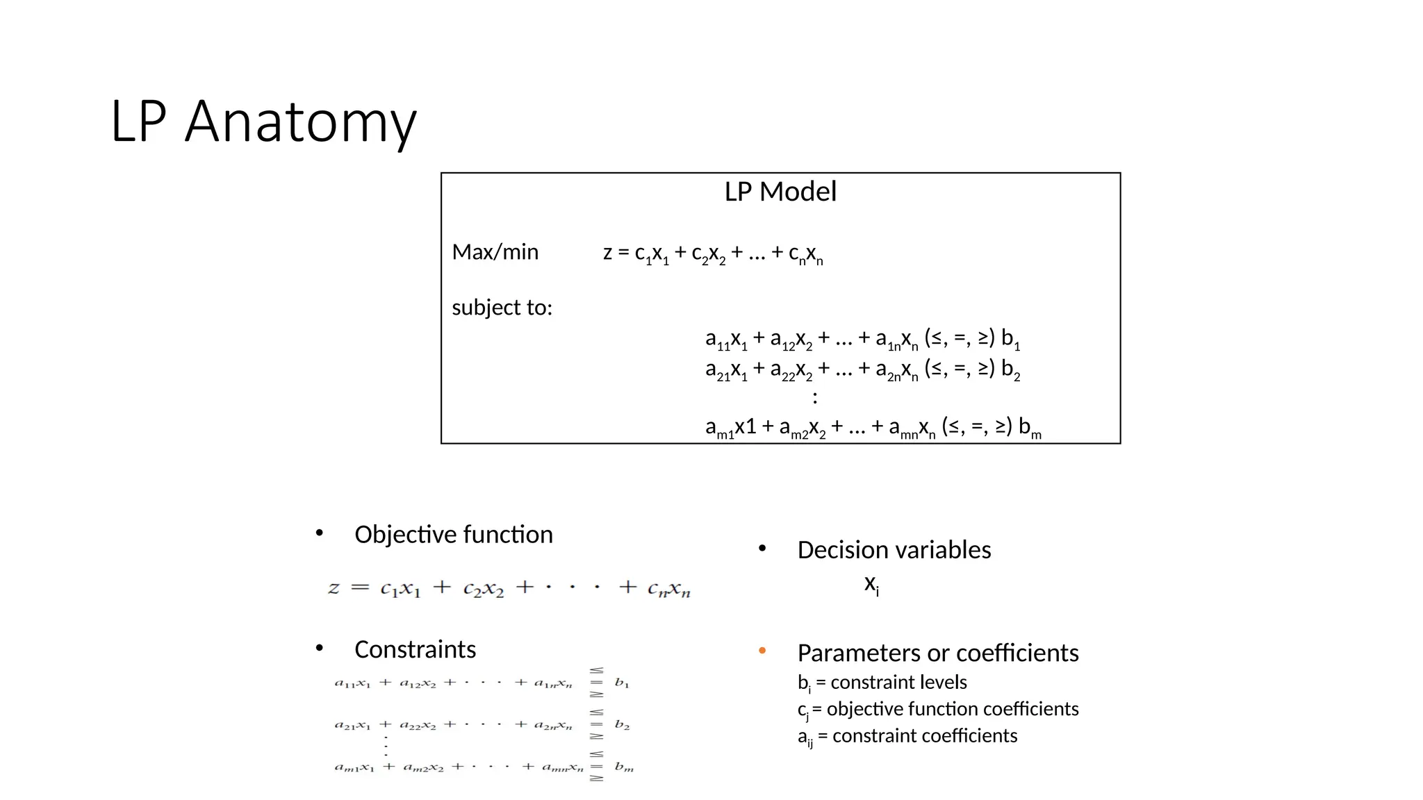
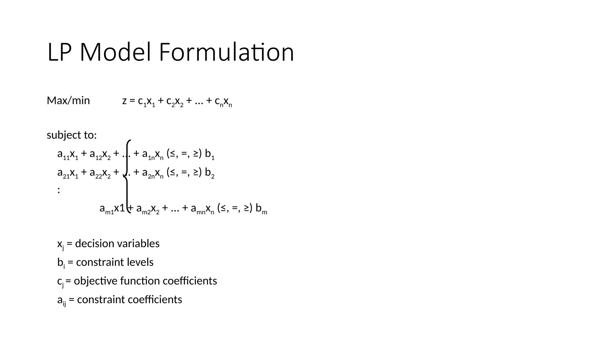
Linear Programming
Lecture Outline
• Background and Definition of LP
• Linear Programming Model
• Graphical Solution Method
• Simplex Method
• A model consisting of linear relationships representing a firm’s objective
and resource constraints.
• A model, which is used for optimum allocation of scarce or limited
resources to competing products or activities under such assumptions as
certainty, linearity, fixed technology, and constant profit per unit.
• LP is a mathematical modeling technique used to determine a level of
operational activity in order to achieve an objective, subject to restrictions
called constraints
Linear Programming (LP)
Any linear programming model (problem) must have the following
properties:
(a) The relationship between variables and constraints must be linear.
(b) The model must have an objective function.
(c) The model must have structural constraints.
(d) The model must have non-negativity constraint.
Properties of Linear Programming
Assumptions in LP
• Proportionality. With linear programs, we assume that the
contribution of
individual variables in the objective function and constraints is
proportional to their value.
• Additivity. Additivity means that the total value of the
objective function and each constraint function is obtained by
adding up the individual contributions from each variable.
• Divisibility. The decision variables are allowed to take on any
real numerical values within some range specified by the
constraints.
• Certainty. We assume that the parameter values in the model
are known with certainty or are at least treated that way.
Applications of LP
Applications of LP
Aggregate Production
Planning
Determines the resource capacity
needed to meet demand over immediate
time horizon, including units produced,
workers hired and fired and inventory
Applications of LP
Product Mix
Mix of different products to produce that will
maximize profit or minimize cost given resource constraints
such as material, labor, budget, etc
Applications of LP
Transportation
Logistical flow of items (goods or services) from
sources to destinations, for example, truckloads of goods
from plants to warehouses
Applications of LP
Transshipment
Flow of items from sources to destinations with
intermediate points, for example shipping from plant to
distribution center and then to stores.
Applications of LP (cont.)
LP Model Formulation
• Decision variables
• mathematical symbols representing levels of activity of an operation
• Physical quantities controlled by the decision maker and represented by
mathematical symbols.
• Objective function
• a linear relationship reflecting the objective of an operation
• Criterion for evaluating the solution.
• Function to be optimized (minimize or maximize)
• Constraints
• a linear relationship representing a restriction on decision making
• A set of functional equalities or inequalities that represent physical,
economic, technological, legal, ethical, or other restrictions on what
numerical values can be assigned to the decision variables.
LP Anatomy
LP Model
Max/min z = c1x1 + c2x2 + ... + cnxn
subject to:
a11x1 + a12x2 + ... + a1nxn (≤, =, ≥) b1
a21x1 + a22x2 + ... + a2nxn (≤, =, ≥) b2
:
am1x1 + am2x2 + ... + amnxn (≤, =, ≥) bm
• Parameters or coefficients
bi = constraint levels
cj = objective function coefficients
aij = constraint coefficients
• Decision variables
xi
• Objective function
• Constraints
LP Model Formulation
Max/min z = c1x1 + c2x2 + ... + cnxn
subject to:
a11x1 + a12x2 + ... + a1nxn (≤, =, ≥) b1
a21x1 + a22x2 + ... + a2nxn (≤, =, ≥) b2
:
am1x1 + am2x2 + ... + amnxn (≤, =, ≥) bm
xj = decision variables
bi = constraint levels
cj = objective function coefficients
aij = constraint coefficients
Steps in LP Modelling
• Identify and define the decision variables for the problem. Define the
variables
completely and precisely. All units of measure need to be stated explicitly,
including time units if appropriate.
• Define the objective function. Determine the criterion for evaluating
alternative solutions. The objective function will normally be the sum of terms
made up of a variable multiplied by some appropriate coefficient (parameter).
• Identify and express mathematically all of the relevant constraints. It is often
easier to express each constraint in words before putting it into mathematical
form.
Let’s Do the Modeling!!!
Example 1: Textile Industry
A retail store stocks two types of shirts A and B. These are packed in attractive
cardboard boxes. During a week the store can sell a maximum of 400 shirts of type A and a
maximum of 300 shirts of type B. The storage capacity, however, is limited to a maximum of
600 of both types combined. Type A shirt fetches a profit of $2 per unit and type B a profit
of $5 per unit. How many of each type the store should stock per week to maximize the total
profit? Formulate a mathematical model of the problem.
Example 2: Manufacturing
A company manufactures two products X and Y, which require, the following
resources. The resources are the capacities machine M1, M2, and M3. The available
capacities are 50,25,and 15 hours respectively in the planning period. Product X requires 1
hour of machine M2 and 1 hour of machine M3. Product Y requires 2 hours of machine M1,
2 hours of machine M2 and 1 hour of machine M3. The profit contribution of products X
and Y are $5 and $4, respectively.
Example 3: Agriculture
International Wool Company operates a large farm on which
sheep are raised. The farm manager determined that for the sheep to
grow in the desired fashion, they need at least minimum amounts of
four nutrients (the nutrients are nontoxic so the sheep can consume
more than the minimum without harm). The manager is considering
three different grains to feed the sheep. Table B-2 lists the number of
units of each nutrient in each pound of grain, the minimum daily
requirements of each nutrient for each sheep, and the cost of each
grain. The manager believes that as long as a sheep receives the
minimum daily amount of each nutrient, it will be healthy and produce
a standard amount of wool. The manager wants to raise the sheep at
minimum cost.
International Wool Company operates a large farm on which sheep are raised. The
farm manager determined that for the sheep to grow in the desired fashion, they need at
least minimum amounts of four nutrients (the nutrients are nontoxic so the sheep can
consume more than the minimum without harm). The manager is considering three
different grains to feed the sheep. Table B-2 lists the number of units of each nutrient in
each pound of grain, the minimum daily requirements of each nutrient for each sheep, and
the cost of each grain. The manager believes that as long as a sheep receives the minimum
daily amount of each nutrient, it will be healthy and produce a standard amount of wool.
The manager wants to raise the sheep at minimum cost.
It’s Your Turn
Practice Problems
1. A company manufactures two products X and Y. The profit contribution of X and Y are $3 and
$4 respectively. The products X and Y require the services of four facilities. The capacities of
the four facilities A, B, C, and D are limited and the available capacities in hours are 200 Hrs,
150 Hrs, and 100 Hrs. and 80 hours respectively. Product X requires 5, 3, 5 and 8 hours of
facilities A, B, C and D respectively. Similarly, the requirement of product Y is 4, 5, 5, and 4
hours respectively on A, B, C and D. Find the optimal product mix to maximize the profit.
2. The cost of materials A and B is $1 per unit respectively. We have to manufacture an alloy by
mixing these to materials. The process of preparing the alloy is carried out on three facilities X,
Y and Z. Facilities X and Z are machines, whose capacities are limited. Y is a furnace, where heat
treatment takes place and the material must use a minimum given time (even if it uses more than
the required, there is no harm). Material A requires 5 hours of machine X and it does not require
processing on machine Z. Material B requires 10 hours of machine X and 1 hour of machine Z.
Both A and B are to be heat treated at last one hour in furnace Y. The available capacities of X, Y
and Z are 50 hours, 1 hour and 4 hours respectively. Find how much of A and B are mixed so as
to minimize the cost
Solution to Linear Programming Problems
Graphical Method
Graphical Solution Method
1. Plot model constraint on a set of coordinates in a plane
2. Identify the feasible solution space on the graph where
all constraints are satisfied simultaneously
3. Plot objective function to find the point on boundary of
this space that maximizes (or minimizes) value of
objective function
Graphical Solution: Example
4 x1 + 3 x2 120 lb
x1 + 2 x2 40 hr
Area common to
both constraints
50 –
40 –
30 –
20 –
10 –
0 –
|
10
|
60
|
50
|
20
|
30
|
40 x1
x2
Computing Optimal Values
x1 + 2x2 = 40
4x1 + 3x2 = 120
4x1 + 8x2 = 160
-4x1 - 3x2 = -120
5x2 = 40
x2 = 8
x1 + 2(8) = 40
x1 = 24
4 x1 + 3 x2 120 lb
x1 + 2 x2 40 hr
40 –
30 –
20 –
10 –
0 –
|
10
|
20
|
30
|
40
x1
x2
Z = $50(24) + $50(8) = $1,360
24
8
Extreme Corner Points
x1 = 224 bowls
x2 =8 mugs
Z = $1,360 x1 = 30 bowls
x2 =0 mugs
Z = $1,200
x1 = 0 bowls
x2 =20 mugs
Z = $1,000
A
B
C
|
20
|
30
|
40
|
10 x1
x2
40 –
30 –
20 –
10 –
0 –
4x1 + 3x2 120 lb
x1 + 2x2 40 hr
40 –
30 –
20 –
10 –
0 –
B
|
10
|
20
|
30
|
40 x1
x2
C
A
Z = 70x1 + 20x2
Optimal point:
x1 = 30 bowls
x2 =0 mugs
Z = $2,100
Objective Function
Minimization Problem
CHEMICAL CONTRIBUTION
Brand Nitrogen (lb/bag) Phosphate (lb/bag)
Gro-plus 2 4
Crop-fast 4 3
Minimize Z = $6x1 + $3x2
subject to
2x1 + 4x2  16 lb of nitrogen
4x1 + 3x2  24 lb of phosphate
x1, x2  0
Copyright 2006 John Wiley & Sons, Inc. Supplement 13-32
14 –
12 –
10 –
8 –
6 –
4 –
2 –
0 –
|
2
|
4
|
6
|
8
|
10
|
12
|
14 x1
x2
A
B
C
Graphical Solution
x1 = 0 bags of Gro-plus
x2 = 8 bags of Crop-fast
Z = $24
Z = 6x1 + 3x2
Copyright 2006 John Wiley & Sons, Inc. Supplement 13-33
Simplex Method
• A mathematical procedure for solving linear programming problems
according to a set of steps
• Slack variables added to ≤ constraints to represent unused resources
• x1 + 2x2 + s1 =40 hours of labor

• 4x1 + 3x2 + s2 =120 lb of clay

• Surplus variables subtracted from ≥ constraints to represent excess
above resource requirement. For example
• 2x1 + 4x2 ≥ 16 is transformed into

• 2x1 + 4x2 - s1 = 16

• Slack/surplus variables have a 0 coefficient in the objective function
• Z = $40x1 + $50x2 + 0s1 + 0s2
Copyright 2006 John Wiley & Sons, Inc. Supplement 13-34
Solution
Points with
Slack
Variables
Solution
Points with
Surplus
Variables
Problem 2.5. A machine tool company conducts a job-training
programme at a ratio of one for every
ten trainees. The training programme lasts for one month. From
past experience it has been found that
out of 10 trainees hired, only seven complete the programme
successfully. (The unsuccessful trainees
are released). Trained machinists are also needed for machining.
The company's requirement for the
next three months is as follows:
January: 100 machinists, February: 150 machinists and March:
200 machinists.
In addition, the company requires 250 trained machinists by
April. There are 130 trained machinists
available at the beginning of the year. Pay roll cost per month
is:
Each trainee Rs. 400/- per month.
Each trained machinist (machining or teaching): Rs. 700/- p.m.
Each trained machinist who is idle: Rs.500/- p.m.
(Labour union forbids ousting trained machinists). Build a l.p.p.
for produce the minimum cost
hiring and training schedule and meet the company’s
requirement.
A ship has three cargo holds, forward, aft and center. The capacity limits are:
Forward 2000 tons, 100,000 cubic meters
Center 3000 tons, 135,000 cubic meters
Aft 1500 tons, 30,000 cubic meters.
The following cargoes are offered, the ship owners may accept all or any part of
each commodity:
Commodity Amount in tons. Volume/ton in cubic meters Profit per ton in Rs.
A 6000 60 60
B 4000 50 80
C 2000 25 50
26 Operations Research
In order to preserve the trim of the ship the weight in each hold must be
proportional to the
capacity in tons. How should the cargo be distributed so as to maximize profit?
Formulate this as linear
programming problem.
Simplex Method- exercises
• 1) A company produces 3 different products: A, B and C. Each product has to go under 3
processes consuming different amounts of time along the way. The time available for
each process is described in the table below.
Assuming the selling profits for products A, B and C are 2, 3 and 4€ per unit. Determine
how many units of each product should be produced to maximize the profit.
Was there any time left?
Process Total number of
hours available
Number of hours needed to produce each
product
A B C
I 12000 5 2 4
II 24000 4 5 6
III 18000 3 5 4
Simplex Method- exercises
• 2) A company produces 3 diferente bookshelves: a luxury, a regular and na exportation
model. Consider the maximum demand for each model to be 500, 750 and 400
respectively. The working hours at the carpentry and finishing sections have the working
time limitations below:
Assuming the selling profit for the luxury, regular and exportation models is 1500, 1300
2500 respectively, formulate the LP problema in order to maximize the profit.
Interpret the results detailling the optimal number of bookshelves of each type produced
discussing the total amount of hours used in each section. How far from meeting the
maximum demands were we?
Section Total
number of
hours
(thousands)
Number of hours needed to produce each
model
luxury regular exportation
carpentry 1.4 0.5 0.5 1.0
finishing 1.2 0.5 0.5 2.0
Simplex Method- exercises
• 3) Max: Z = x1 + 2 x2
Subject to:
2x1 + 4x2 ≤ 20
x1 + x2 ≤ 8
and x1 x2 ≥ 0
• 4) Max: Z = x1 + x2
Subject to:
x1 + x2 ≤ 4
2 x1 + x2 ≤ 6
x1 + 2 x2 ≤ 6
and x1 x2 ≥ 0
• 5) Max: Z = x1 + x2
Subject to:
x1 + x2 ≤ 10
2 x1 - 3 x2 ≤ 15
x1 - 2 x2 ≤ 20
and x1 x2 ≥ 0
Apply the Simplex to find the optimal solution
Multiple, unbound and degenerate solutions
Simplex Method- exercises
Max: Z = 10 x1 + 30 x2
Subject to:
x1 ≤ 15
x1 - x2 ≤ 20
-3 x1 + x2 ≤ -30
and x1 ≥ 0 x2 ≤ 0
• 7)
• 8)
Bring the following PL problems to standard form and apply the
Simplex to find the optimal solution
Minimization, negative RHS, negative and unbounded variables
• 6) Min: Z = 2 x1 - 3 x2 – 4 x3
Subject to:
x1 + 5x2 -3x3 ≤ 15
x1 + x2 + x3 ≤ 11
5 x1 – 6 x2 + x3 ≤ 4
and x1 x2 x3 ≥ 0
Max: Z = - x2
Subject to:
x1 + x2 + x3 ≤ 100
x1 - 5 x2 ≤ 40
x3 ≥ -10
and x1 ≥ 0 x2 ≤ 0 x3 unbounded
Simplex Method- exercises
• 10)
Bring the following PL problems to standard form introducing artificial
variables apply the big M method using Simplex to find the optimal
solutions
• 9) Max: Z = x1 + 2 x2
Subject to: x1 + x2 ≤ 10
x1 - 2 x2 ≥ 6
x1, x2 ≥ 0
Min: Z = 4 x1 + 2 x2
Subject to: 2 x1 - x2 ≥ 4
x1 + x2 ≥ 5
x1, x2 ≥ 0
Given the following linear programming model:
Min Z=4x1+x2
s.t.
3x1+6x2>=15
8x1+2x2>=12
x1, x2>=0
Solve graphically and using the simplex method.
What type of special case is this problem? Explain?
3. Transform the following linear programming model into proper form
and setup the initial tableau. Do not solve it.
Min Z=40x1+55x2+30x3
s.t.
x1+2x2+3x3 <=60
2x1+x2+x3 = 40
x1+3x2+x3>=50
5x2+x3>=100
x1, x2, x3>=0
4. Given the following linear programming model:
Max Z=x1+2x2-x3
s.t.
4x2+x3<=40
x1-x2<=20
2x1+4x2+3x3<=60
x1, x2, x3>=0
Solve this problem using the simplex method.
What type of special case is this problem? Explain?
Worked Out Problems
47
Example Problem
Maximize Z = 5x1 + 2x2 + x3
subject to
x1 + 3x2 - x3 ≤ 6,
x2 + x3 ≤ 4,
3x1 + x2 ≤ 7,
x1, x2, x3 ≥ 0.
48
Simplex and Example Problem
Step 1. Convert to Standard Form
a11 x1 + a12 x2 + ••• + a1n xn ≤ b1,
a21 x1 + a22 x2 + ••• + a2n xn ≥ b2,
am1 x1 + am2 x2 + ••• + amn xn ≤ bm,

a11 x1 + a12 x2 + ••• + a1n xn + xn+1 = b1,
a21 x1 + a22 x2 + ••• + a2n xn - xn+2 = b2,
am1 x1 + am2 x2 + ••• + amn xn + xn+k = bm,
In our example problem:
x1 + 3x2 - x3 ≤ 6,
x2 + x3 ≤ 4,
3x1 + x2 ≤ 7,
x1, x2, x3 ≥ 0.
x1 + 3x2 - x3 + x4 = 6,
x2 + x3 + x5 = 4,
3x1 + x2 + x6 = 7,
x1, x2, x3, x4, x5, x6 ≥ 0.
49
Simplex: Step 2
Step 2. Start with an initial basic feasible solution (b.f.s.) and set up the initial
tableau.
In our example
Maximize Z = 5x1 + 2x2 + x3
x1 + 3x2 - x3 + x4 = 6,
x2 + x3 + x5 = 4,
3x1 + x2 + x6 = 7,
x1, x2, x3, x4, x5, x6 ≥ 0.
c
j
5
2
1
0
0
0
c
B
B
a
s
i
s
x
1
x
2
x
3
x
4
x
5
x
6
C
o
n
s
t
a
n
t
s
0x
4 1
3
-
1
1
0
0 6
0x
5 0
1
1
0
1
0 4
0x
6 3
1
0
0
0
1 7
c
r
o
w
5
2
1
0
0
0 Z
=
0
50
Step 2: Explanation
Adjacent Basic Feasible Solution
If we bring a nonbasic variable xs into the basis, our system changes from the basis,
xb, to the following (same notation as the book):
x1 + ā1sxs=
xr + ārsxr=
xm + āmsxs=
1
b
r
b
s
b


xi = for i =1, …, m
is
i a
b 
xs = 1
xj = 0 for j=m+1, ..., n and js
The new value of the objective function becomes:





m
1
i
s
is
i
i c
)
a
b
(
c
Z
Thus the change in the value of Z per unit increase in xs is
s
c = new value of Z - old value of Z
= 
 




m
1
i
i
i
m
1
i
s
is
i
i b
c
c
)
a
b
(
c



m
1
i
is
i
s a
c
c
=
This is the Inner Product rule
51
Simplex: Step 3
Use the inner product rule to find the relative profit coefficients
c
j
5
2
1
0
0
0
c
B
B
a
s
i
s
x
1
x
2
x
3
x
4
x
5
x
6
C
o
n
s
t
a
n
t
s
0x
4 1
3
-
1
1
0
0 6
0x
5 0
1
1
0
1
0 4
0x
6 3
1
0
0
0
1 7
c
r
o
w
5
2
1
0
0
0 Z
=
0
j
B
j
j P
c
c
c 

c1 = 5 - 0(1) - 0(0) - 0(3) = 5 -> largest positive
c2 = ….
c3 = ….
Step 4: Is this an optimal basic feasible solution?
52
Simplex: Step 5
Apply the minimum ratio rule to determine the basic variable to leave the basis.
The new values of the basis variables:
xi = for i = 1, ..., m
s
is
i x
a
b 







 is
i
0
a
s
a
b
min
x
max
is
In our example:
c
j
5
2
1
0
0
0
c
B
B
a
s
i
s
x
1
x
2
x
3
x
4
x
5
x
6
C
o
n
s
t
a
n
t
s
0x
4 1
3
-
1
1
0
0 6
0x
5 0
1
1
0
1
0 4
0x
6 3
1
0
0
0
1 7
c
r
o
w
5
2
1
0
0
0 Z
=
0
Row Basic Variable Ratio
1 x4 6
2 x5 -
3 x6 7/3
53
c
j
5
2
1
0
0
0
c
B
B
a
s
i
s
x
1x
2
x
3
x
4
x
5x
6
C
o
n
s
t
a
n
t
s
0x
4 0
8
/
3
-
1
1
0
0 1
1
/
3
0x
5 0
1
1
0
1
0 4
5x
1 1
1
/
3
0
0
0
1
/
37
/
3
c
r
o
w
0
1
/
3
1
0
0
-
5
/
3
Z
=
3
5
/
3
Simplex: Step 6
Perform the pivot operation to get the new tableau and the b.f.s.
c
j
5
2
1
0
0
0
c
B
B
a
s
i
s
x
1
x
2
x
3
x
4
x
5
x
6
C
o
n
s
t
a
n
t
s
0x
4 1
3
-
1
1
0
0 6
0x
5 0
1
1
0
1
0 4
0x
6 3
1
0
0
0
1 7
c
r
o
w
5
2
1
0
0
0Z
=
0
j
B
j
j P
c
c
c 

c2 = 2 - (0) 8/3 - (0) 1 - (5) 1/3 = 1/3
c3 = 1 - (0) (-1) - (0) 1 - (5) 0 = 1
c6 = 0 - (0) 0 - (0) 0 - (5) 1/3 = -5/3
cB = (0 0 5)
New iteration:
find entering
variable:
54
Final Tableau
c
j
5
2
1
0
0
0
c
B
B
a
s
i
s
x
1x
2
x
3
x
4
x
5x
6
C
o
n
s
t
a
n
t
s
0x
4 0
8
/
3
-
1
1
0
0 1
1
/
3
0x
5 0
1
1
0
1
0 4
5x
1 1
1
/
3
0
0
0
1
/
37
/
3
c
r
o
w
0
1
/
3
1
0
0
-
5
/
3
Z
=
3
5
/
3
c
j
5
2
1
0
0
0
c
B
B
a
s
i
s
x
1x
2x
3
x
4
x
5x
6
C
o
n
s
t
a
n
t
s
0x
4 0
4
0
1
1
0 2
3
/
3
1x
3 0
1
1
0
1
0 4
5x
1 1
1
/
3
0
0
0
1
/
37
/
3
c
r
o
w
0
-
2
/
3
0
0
-
1
-
5
/
3
Z
=
4
7
/
3
x3 enters basis,
x5 leaves basis
Wrong value!
4 should be 11/3

Unit 3 Lesson 1 - Linear Programming Lecture.pptx

  • 1.
  • 2.
    Lecture Outline • Backgroundand Definition of LP • Linear Programming Model • Graphical Solution Method • Simplex Method
  • 3.
    • A modelconsisting of linear relationships representing a firm’s objective and resource constraints. • A model, which is used for optimum allocation of scarce or limited resources to competing products or activities under such assumptions as certainty, linearity, fixed technology, and constant profit per unit. • LP is a mathematical modeling technique used to determine a level of operational activity in order to achieve an objective, subject to restrictions called constraints Linear Programming (LP)
  • 4.
    Any linear programmingmodel (problem) must have the following properties: (a) The relationship between variables and constraints must be linear. (b) The model must have an objective function. (c) The model must have structural constraints. (d) The model must have non-negativity constraint. Properties of Linear Programming
  • 5.
    Assumptions in LP •Proportionality. With linear programs, we assume that the contribution of individual variables in the objective function and constraints is proportional to their value. • Additivity. Additivity means that the total value of the objective function and each constraint function is obtained by adding up the individual contributions from each variable. • Divisibility. The decision variables are allowed to take on any real numerical values within some range specified by the constraints. • Certainty. We assume that the parameter values in the model are known with certainty or are at least treated that way.
  • 6.
  • 7.
    Applications of LP AggregateProduction Planning Determines the resource capacity needed to meet demand over immediate time horizon, including units produced, workers hired and fired and inventory
  • 8.
    Applications of LP ProductMix Mix of different products to produce that will maximize profit or minimize cost given resource constraints such as material, labor, budget, etc
  • 9.
    Applications of LP Transportation Logisticalflow of items (goods or services) from sources to destinations, for example, truckloads of goods from plants to warehouses
  • 10.
    Applications of LP Transshipment Flowof items from sources to destinations with intermediate points, for example shipping from plant to distribution center and then to stores.
  • 11.
  • 12.
  • 13.
    LP Model Formulation •Decision variables • mathematical symbols representing levels of activity of an operation • Physical quantities controlled by the decision maker and represented by mathematical symbols. • Objective function • a linear relationship reflecting the objective of an operation • Criterion for evaluating the solution. • Function to be optimized (minimize or maximize) • Constraints • a linear relationship representing a restriction on decision making • A set of functional equalities or inequalities that represent physical, economic, technological, legal, ethical, or other restrictions on what numerical values can be assigned to the decision variables.
  • 14.
    LP Anatomy LP Model Max/minz = c1x1 + c2x2 + ... + cnxn subject to: a11x1 + a12x2 + ... + a1nxn (≤, =, ≥) b1 a21x1 + a22x2 + ... + a2nxn (≤, =, ≥) b2 : am1x1 + am2x2 + ... + amnxn (≤, =, ≥) bm • Parameters or coefficients bi = constraint levels cj = objective function coefficients aij = constraint coefficients • Decision variables xi • Objective function • Constraints
  • 15.
    LP Model Formulation Max/minz = c1x1 + c2x2 + ... + cnxn subject to: a11x1 + a12x2 + ... + a1nxn (≤, =, ≥) b1 a21x1 + a22x2 + ... + a2nxn (≤, =, ≥) b2 : am1x1 + am2x2 + ... + amnxn (≤, =, ≥) bm xj = decision variables bi = constraint levels cj = objective function coefficients aij = constraint coefficients
  • 16.
    Steps in LPModelling
  • 17.
    Steps in LPModelling • Identify and define the decision variables for the problem. Define the variables completely and precisely. All units of measure need to be stated explicitly, including time units if appropriate. • Define the objective function. Determine the criterion for evaluating alternative solutions. The objective function will normally be the sum of terms made up of a variable multiplied by some appropriate coefficient (parameter). • Identify and express mathematically all of the relevant constraints. It is often easier to express each constraint in words before putting it into mathematical form.
  • 18.
    Let’s Do theModeling!!!
  • 19.
    Example 1: TextileIndustry A retail store stocks two types of shirts A and B. These are packed in attractive cardboard boxes. During a week the store can sell a maximum of 400 shirts of type A and a maximum of 300 shirts of type B. The storage capacity, however, is limited to a maximum of 600 of both types combined. Type A shirt fetches a profit of $2 per unit and type B a profit of $5 per unit. How many of each type the store should stock per week to maximize the total profit? Formulate a mathematical model of the problem.
  • 20.
    Example 2: Manufacturing Acompany manufactures two products X and Y, which require, the following resources. The resources are the capacities machine M1, M2, and M3. The available capacities are 50,25,and 15 hours respectively in the planning period. Product X requires 1 hour of machine M2 and 1 hour of machine M3. Product Y requires 2 hours of machine M1, 2 hours of machine M2 and 1 hour of machine M3. The profit contribution of products X and Y are $5 and $4, respectively.
  • 21.
    Example 3: Agriculture InternationalWool Company operates a large farm on which sheep are raised. The farm manager determined that for the sheep to grow in the desired fashion, they need at least minimum amounts of four nutrients (the nutrients are nontoxic so the sheep can consume more than the minimum without harm). The manager is considering three different grains to feed the sheep. Table B-2 lists the number of units of each nutrient in each pound of grain, the minimum daily requirements of each nutrient for each sheep, and the cost of each grain. The manager believes that as long as a sheep receives the minimum daily amount of each nutrient, it will be healthy and produce a standard amount of wool. The manager wants to raise the sheep at minimum cost.
  • 22.
    International Wool Companyoperates a large farm on which sheep are raised. The farm manager determined that for the sheep to grow in the desired fashion, they need at least minimum amounts of four nutrients (the nutrients are nontoxic so the sheep can consume more than the minimum without harm). The manager is considering three different grains to feed the sheep. Table B-2 lists the number of units of each nutrient in each pound of grain, the minimum daily requirements of each nutrient for each sheep, and the cost of each grain. The manager believes that as long as a sheep receives the minimum daily amount of each nutrient, it will be healthy and produce a standard amount of wool. The manager wants to raise the sheep at minimum cost.
  • 23.
  • 24.
    Practice Problems 1. Acompany manufactures two products X and Y. The profit contribution of X and Y are $3 and $4 respectively. The products X and Y require the services of four facilities. The capacities of the four facilities A, B, C, and D are limited and the available capacities in hours are 200 Hrs, 150 Hrs, and 100 Hrs. and 80 hours respectively. Product X requires 5, 3, 5 and 8 hours of facilities A, B, C and D respectively. Similarly, the requirement of product Y is 4, 5, 5, and 4 hours respectively on A, B, C and D. Find the optimal product mix to maximize the profit. 2. The cost of materials A and B is $1 per unit respectively. We have to manufacture an alloy by mixing these to materials. The process of preparing the alloy is carried out on three facilities X, Y and Z. Facilities X and Z are machines, whose capacities are limited. Y is a furnace, where heat treatment takes place and the material must use a minimum given time (even if it uses more than the required, there is no harm). Material A requires 5 hours of machine X and it does not require processing on machine Z. Material B requires 10 hours of machine X and 1 hour of machine Z. Both A and B are to be heat treated at last one hour in furnace Y. The available capacities of X, Y and Z are 50 hours, 1 hour and 4 hours respectively. Find how much of A and B are mixed so as to minimize the cost
  • 25.
    Solution to LinearProgramming Problems Graphical Method
  • 26.
    Graphical Solution Method 1.Plot model constraint on a set of coordinates in a plane 2. Identify the feasible solution space on the graph where all constraints are satisfied simultaneously 3. Plot objective function to find the point on boundary of this space that maximizes (or minimizes) value of objective function
  • 27.
    Graphical Solution: Example 4x1 + 3 x2 120 lb x1 + 2 x2 40 hr Area common to both constraints 50 – 40 – 30 – 20 – 10 – 0 – | 10 | 60 | 50 | 20 | 30 | 40 x1 x2
  • 28.
    Computing Optimal Values x1+ 2x2 = 40 4x1 + 3x2 = 120 4x1 + 8x2 = 160 -4x1 - 3x2 = -120 5x2 = 40 x2 = 8 x1 + 2(8) = 40 x1 = 24 4 x1 + 3 x2 120 lb x1 + 2 x2 40 hr 40 – 30 – 20 – 10 – 0 – | 10 | 20 | 30 | 40 x1 x2 Z = $50(24) + $50(8) = $1,360 24 8
  • 29.
    Extreme Corner Points x1= 224 bowls x2 =8 mugs Z = $1,360 x1 = 30 bowls x2 =0 mugs Z = $1,200 x1 = 0 bowls x2 =20 mugs Z = $1,000 A B C | 20 | 30 | 40 | 10 x1 x2 40 – 30 – 20 – 10 – 0 –
  • 30.
    4x1 + 3x2120 lb x1 + 2x2 40 hr 40 – 30 – 20 – 10 – 0 – B | 10 | 20 | 30 | 40 x1 x2 C A Z = 70x1 + 20x2 Optimal point: x1 = 30 bowls x2 =0 mugs Z = $2,100 Objective Function
  • 31.
    Minimization Problem CHEMICAL CONTRIBUTION BrandNitrogen (lb/bag) Phosphate (lb/bag) Gro-plus 2 4 Crop-fast 4 3 Minimize Z = $6x1 + $3x2 subject to 2x1 + 4x2  16 lb of nitrogen 4x1 + 3x2  24 lb of phosphate x1, x2  0
  • 32.
    Copyright 2006 JohnWiley & Sons, Inc. Supplement 13-32 14 – 12 – 10 – 8 – 6 – 4 – 2 – 0 – | 2 | 4 | 6 | 8 | 10 | 12 | 14 x1 x2 A B C Graphical Solution x1 = 0 bags of Gro-plus x2 = 8 bags of Crop-fast Z = $24 Z = 6x1 + 3x2
  • 33.
    Copyright 2006 JohnWiley & Sons, Inc. Supplement 13-33 Simplex Method • A mathematical procedure for solving linear programming problems according to a set of steps • Slack variables added to ≤ constraints to represent unused resources • x1 + 2x2 + s1 =40 hours of labor  • 4x1 + 3x2 + s2 =120 lb of clay  • Surplus variables subtracted from ≥ constraints to represent excess above resource requirement. For example • 2x1 + 4x2 ≥ 16 is transformed into  • 2x1 + 4x2 - s1 = 16  • Slack/surplus variables have a 0 coefficient in the objective function • Z = $40x1 + $50x2 + 0s1 + 0s2
  • 34.
    Copyright 2006 JohnWiley & Sons, Inc. Supplement 13-34 Solution Points with Slack Variables
  • 35.
  • 38.
    Problem 2.5. Amachine tool company conducts a job-training programme at a ratio of one for every ten trainees. The training programme lasts for one month. From past experience it has been found that out of 10 trainees hired, only seven complete the programme successfully. (The unsuccessful trainees are released). Trained machinists are also needed for machining. The company's requirement for the next three months is as follows: January: 100 machinists, February: 150 machinists and March: 200 machinists. In addition, the company requires 250 trained machinists by April. There are 130 trained machinists available at the beginning of the year. Pay roll cost per month is: Each trainee Rs. 400/- per month. Each trained machinist (machining or teaching): Rs. 700/- p.m. Each trained machinist who is idle: Rs.500/- p.m. (Labour union forbids ousting trained machinists). Build a l.p.p. for produce the minimum cost hiring and training schedule and meet the company’s requirement.
  • 39.
    A ship hasthree cargo holds, forward, aft and center. The capacity limits are: Forward 2000 tons, 100,000 cubic meters Center 3000 tons, 135,000 cubic meters Aft 1500 tons, 30,000 cubic meters. The following cargoes are offered, the ship owners may accept all or any part of each commodity: Commodity Amount in tons. Volume/ton in cubic meters Profit per ton in Rs. A 6000 60 60 B 4000 50 80 C 2000 25 50 26 Operations Research In order to preserve the trim of the ship the weight in each hold must be proportional to the capacity in tons. How should the cargo be distributed so as to maximize profit? Formulate this as linear programming problem.
  • 40.
    Simplex Method- exercises •1) A company produces 3 different products: A, B and C. Each product has to go under 3 processes consuming different amounts of time along the way. The time available for each process is described in the table below. Assuming the selling profits for products A, B and C are 2, 3 and 4€ per unit. Determine how many units of each product should be produced to maximize the profit. Was there any time left? Process Total number of hours available Number of hours needed to produce each product A B C I 12000 5 2 4 II 24000 4 5 6 III 18000 3 5 4
  • 41.
    Simplex Method- exercises •2) A company produces 3 diferente bookshelves: a luxury, a regular and na exportation model. Consider the maximum demand for each model to be 500, 750 and 400 respectively. The working hours at the carpentry and finishing sections have the working time limitations below: Assuming the selling profit for the luxury, regular and exportation models is 1500, 1300 2500 respectively, formulate the LP problema in order to maximize the profit. Interpret the results detailling the optimal number of bookshelves of each type produced discussing the total amount of hours used in each section. How far from meeting the maximum demands were we? Section Total number of hours (thousands) Number of hours needed to produce each model luxury regular exportation carpentry 1.4 0.5 0.5 1.0 finishing 1.2 0.5 0.5 2.0
  • 42.
    Simplex Method- exercises •3) Max: Z = x1 + 2 x2 Subject to: 2x1 + 4x2 ≤ 20 x1 + x2 ≤ 8 and x1 x2 ≥ 0 • 4) Max: Z = x1 + x2 Subject to: x1 + x2 ≤ 4 2 x1 + x2 ≤ 6 x1 + 2 x2 ≤ 6 and x1 x2 ≥ 0 • 5) Max: Z = x1 + x2 Subject to: x1 + x2 ≤ 10 2 x1 - 3 x2 ≤ 15 x1 - 2 x2 ≤ 20 and x1 x2 ≥ 0 Apply the Simplex to find the optimal solution Multiple, unbound and degenerate solutions
  • 43.
    Simplex Method- exercises Max:Z = 10 x1 + 30 x2 Subject to: x1 ≤ 15 x1 - x2 ≤ 20 -3 x1 + x2 ≤ -30 and x1 ≥ 0 x2 ≤ 0 • 7) • 8) Bring the following PL problems to standard form and apply the Simplex to find the optimal solution Minimization, negative RHS, negative and unbounded variables • 6) Min: Z = 2 x1 - 3 x2 – 4 x3 Subject to: x1 + 5x2 -3x3 ≤ 15 x1 + x2 + x3 ≤ 11 5 x1 – 6 x2 + x3 ≤ 4 and x1 x2 x3 ≥ 0 Max: Z = - x2 Subject to: x1 + x2 + x3 ≤ 100 x1 - 5 x2 ≤ 40 x3 ≥ -10 and x1 ≥ 0 x2 ≤ 0 x3 unbounded
  • 44.
    Simplex Method- exercises •10) Bring the following PL problems to standard form introducing artificial variables apply the big M method using Simplex to find the optimal solutions • 9) Max: Z = x1 + 2 x2 Subject to: x1 + x2 ≤ 10 x1 - 2 x2 ≥ 6 x1, x2 ≥ 0 Min: Z = 4 x1 + 2 x2 Subject to: 2 x1 - x2 ≥ 4 x1 + x2 ≥ 5 x1, x2 ≥ 0
  • 45.
    Given the followinglinear programming model: Min Z=4x1+x2 s.t. 3x1+6x2>=15 8x1+2x2>=12 x1, x2>=0 Solve graphically and using the simplex method. What type of special case is this problem? Explain? 3. Transform the following linear programming model into proper form and setup the initial tableau. Do not solve it. Min Z=40x1+55x2+30x3 s.t. x1+2x2+3x3 <=60 2x1+x2+x3 = 40 x1+3x2+x3>=50 5x2+x3>=100 x1, x2, x3>=0 4. Given the following linear programming model: Max Z=x1+2x2-x3 s.t. 4x2+x3<=40 x1-x2<=20 2x1+4x2+3x3<=60 x1, x2, x3>=0 Solve this problem using the simplex method. What type of special case is this problem? Explain?
  • 46.
  • 47.
    47 Example Problem Maximize Z= 5x1 + 2x2 + x3 subject to x1 + 3x2 - x3 ≤ 6, x2 + x3 ≤ 4, 3x1 + x2 ≤ 7, x1, x2, x3 ≥ 0.
  • 48.
    48 Simplex and ExampleProblem Step 1. Convert to Standard Form a11 x1 + a12 x2 + ••• + a1n xn ≤ b1, a21 x1 + a22 x2 + ••• + a2n xn ≥ b2, am1 x1 + am2 x2 + ••• + amn xn ≤ bm,  a11 x1 + a12 x2 + ••• + a1n xn + xn+1 = b1, a21 x1 + a22 x2 + ••• + a2n xn - xn+2 = b2, am1 x1 + am2 x2 + ••• + amn xn + xn+k = bm, In our example problem: x1 + 3x2 - x3 ≤ 6, x2 + x3 ≤ 4, 3x1 + x2 ≤ 7, x1, x2, x3 ≥ 0. x1 + 3x2 - x3 + x4 = 6, x2 + x3 + x5 = 4, 3x1 + x2 + x6 = 7, x1, x2, x3, x4, x5, x6 ≥ 0.
  • 49.
    49 Simplex: Step 2 Step2. Start with an initial basic feasible solution (b.f.s.) and set up the initial tableau. In our example Maximize Z = 5x1 + 2x2 + x3 x1 + 3x2 - x3 + x4 = 6, x2 + x3 + x5 = 4, 3x1 + x2 + x6 = 7, x1, x2, x3, x4, x5, x6 ≥ 0. c j 5 2 1 0 0 0 c B B a s i s x 1 x 2 x 3 x 4 x 5 x 6 C o n s t a n t s 0x 4 1 3 - 1 1 0 0 6 0x 5 0 1 1 0 1 0 4 0x 6 3 1 0 0 0 1 7 c r o w 5 2 1 0 0 0 Z = 0
  • 50.
    50 Step 2: Explanation AdjacentBasic Feasible Solution If we bring a nonbasic variable xs into the basis, our system changes from the basis, xb, to the following (same notation as the book): x1 + ā1sxs= xr + ārsxr= xm + āmsxs= 1 b r b s b   xi = for i =1, …, m is i a b  xs = 1 xj = 0 for j=m+1, ..., n and js The new value of the objective function becomes:      m 1 i s is i i c ) a b ( c Z Thus the change in the value of Z per unit increase in xs is s c = new value of Z - old value of Z =        m 1 i i i m 1 i s is i i b c c ) a b ( c    m 1 i is i s a c c = This is the Inner Product rule
  • 51.
    51 Simplex: Step 3 Usethe inner product rule to find the relative profit coefficients c j 5 2 1 0 0 0 c B B a s i s x 1 x 2 x 3 x 4 x 5 x 6 C o n s t a n t s 0x 4 1 3 - 1 1 0 0 6 0x 5 0 1 1 0 1 0 4 0x 6 3 1 0 0 0 1 7 c r o w 5 2 1 0 0 0 Z = 0 j B j j P c c c   c1 = 5 - 0(1) - 0(0) - 0(3) = 5 -> largest positive c2 = …. c3 = …. Step 4: Is this an optimal basic feasible solution?
  • 52.
    52 Simplex: Step 5 Applythe minimum ratio rule to determine the basic variable to leave the basis. The new values of the basis variables: xi = for i = 1, ..., m s is i x a b          is i 0 a s a b min x max is In our example: c j 5 2 1 0 0 0 c B B a s i s x 1 x 2 x 3 x 4 x 5 x 6 C o n s t a n t s 0x 4 1 3 - 1 1 0 0 6 0x 5 0 1 1 0 1 0 4 0x 6 3 1 0 0 0 1 7 c r o w 5 2 1 0 0 0 Z = 0 Row Basic Variable Ratio 1 x4 6 2 x5 - 3 x6 7/3
  • 53.
    53 c j 5 2 1 0 0 0 c B B a s i s x 1x 2 x 3 x 4 x 5x 6 C o n s t a n t s 0x 4 0 8 / 3 - 1 1 0 0 1 1 / 3 0x 50 1 1 0 1 0 4 5x 1 1 1 / 3 0 0 0 1 / 37 / 3 c r o w 0 1 / 3 1 0 0 - 5 / 3 Z = 3 5 / 3 Simplex: Step 6 Perform the pivot operation to get the new tableau and the b.f.s. c j 5 2 1 0 0 0 c B B a s i s x 1 x 2 x 3 x 4 x 5 x 6 C o n s t a n t s 0x 4 1 3 - 1 1 0 0 6 0x 5 0 1 1 0 1 0 4 0x 6 3 1 0 0 0 1 7 c r o w 5 2 1 0 0 0Z = 0 j B j j P c c c   c2 = 2 - (0) 8/3 - (0) 1 - (5) 1/3 = 1/3 c3 = 1 - (0) (-1) - (0) 1 - (5) 0 = 1 c6 = 0 - (0) 0 - (0) 0 - (5) 1/3 = -5/3 cB = (0 0 5) New iteration: find entering variable:
  • 54.
    54 Final Tableau c j 5 2 1 0 0 0 c B B a s i s x 1x 2 x 3 x 4 x 5x 6 C o n s t a n t s 0x 4 0 8 / 3 - 1 1 0 01 1 / 3 0x 5 0 1 1 0 1 0 4 5x 1 1 1 / 3 0 0 0 1 / 37 / 3 c r o w 0 1 / 3 1 0 0 - 5 / 3 Z = 3 5 / 3 c j 5 2 1 0 0 0 c B B a s i s x 1x 2x 3 x 4 x 5x 6 C o n s t a n t s 0x 4 0 4 0 1 1 0 2 3 / 3 1x 3 0 1 1 0 1 0 4 5x 1 1 1 / 3 0 0 0 1 / 37 / 3 c r o w 0 - 2 / 3 0 0 - 1 - 5 / 3 Z = 4 7 / 3 x3 enters basis, x5 leaves basis Wrong value! 4 should be 11/3

Editor's Notes

  • #5 Proportionality. That is, if we double the value of a variable, we double the contribution of that variable to the objective function and each constraint in which the variable appears. The contribution per unit of the variable is constant. For example, suppose the variable xj is the number of units of product j produced and cj is the cost per unit to produce product j. If doubling the amount of product j produced doubles its cost, the per unit cost is constant and the proportionality assumption is satisfied. Divisibility. That is, the variables are not restricted to integer values. When fractional values do not make a sensible solution, such as the number of flights an airline should have each day between two cities, the problem should be formulated and solved as an integer program. Certainty. The optimal solution obtained is optimal for the specific problem formulated. If the parameter values are wrong, then the resulting solution is of little value.
  • #10 and many more
  • #12 Decision variables The decision variable xj can represent the number of pounds of product j that company will produce. Objective function Constraint It ensures that no more input is used than is available.
  • #13 Decision variables The decision variable xj can represent the number of pounds of product j that company will produce. Objective function Constraint It ensures that no more input is used than is available.
  • #14 Decision variables The decision variable xj can represent the number of pounds of product j that company will produce. Objective function Constraint It ensures that no more input is used than is available.
  • #16 Identify and define the decision variables for the problem. For example, if the variables represent quantities of a product produced, these should be defined in terms of tons per hour, units per day, barrels per month, or some other appropriate units. Define the objective function. Determine the criterion for evaluating alternative solutions. The objective function will normally be the sum of terms made up of a variable multiplied by some appropriate coefficient (parameter). For example, the coefficients might be profit per unit of production, distance travel per unit transported, or cost per person hired. Identify and express mathematically all of the relevant constraints. It is often easier to express each constraint in words before putting it into mathematical form. The written constraint is decomposed into its fundamental components. Then substitute the appropriate numerical coefficients and variable names for the written terms. A common mistake is using variables that have not been defined in the problem, which is not valid. This mistake is frequently caused by not defining the original variables precisely.
  • #17 Identify and define the decision variables for the problem. For example, if the variables represent quantities of a product produced, these should be defined in terms of tons per hour, units per day, barrels per month, or some other appropriate units. Define the objective function. Determine the criterion for evaluating alternative solutions. The objective function will normally be the sum of terms made up of a variable multiplied by some appropriate coefficient (parameter). For example, the coefficients might be profit per unit of production, distance travel per unit transported, or cost per person hired. Identify and express mathematically all of the relevant constraints. It is often easier to express each constraint in words before putting it into mathematical form. The written constraint is decomposed into its fundamental components. Then substitute the appropriate numerical coefficients and variable names for the written terms. A common mistake is using variables that have not been defined in the problem, which is not valid. This mistake is frequently caused by not defining the original variables precisely.
  • #19 Maximize Z = 2a + 5b s.t. 1a + 0b ≤ 400 0a + 1b ≤ 300 1a + 1b ≤ 600 and Both a and b are ≥ 0.
  • #20 Maximize Z = 5x + 4y OBJECTIVE FUNCTION. This should be done so that the utilization of machine hours by products x and y should not exceed the available capacity. This can be shown as follows: For Machine M1 0x + 2y ≤ 50 For Machine M2 1x + 2y ≤ 25 and LINEAR STRUCTURAL CONSTRAINTS. For machine M3 1x + 1y ≤ 15 But the company can stop production of x and y or can manufacture any amount of x and y. It cannot manufacture negative quantities of x and y. Hence we have write, Both x and y are ≥ 0 . NON -NEGATIVITY CONSTRAINT.
  • #22 Minimize z 41x1 36x2 96x3 Why can’t the manager simply make all the variables equal to zero? This keeps costs at zero, but the manager would have a flock of dead sheep, because there are minimum nutrient constraints that must be satisfied. The values of the variables must be chosen so that the number of units of nutrient A consumed daily by each sheep is equal to or greater than 110. Expressing this in terms of the variables yields 20x1 30x2 70x3 110 The constraints for the other nutrients are 10x1 10x2 18 50x1 30x2 90 6x1 2.5x2 10x3 110 and finally all xjs 0 The optimal solution to this problem (obtained using a computer software package) is x1 0.595, x2 2.008, x3 0.541, and z 148.6 cents.
  • #24 Maximise Z 3x + 4y S.T. 5x + 4y ≤ 200 3x + 5y ≤ 150 5x + 4y ≤ 100 8x + 4y ≤ 80 And both x and y are ≥ 0 Minimize Z = 1a + 1b S.T. 5a + 10b ≤ 50 1a + 1b ≥ 1 0a + 1b ≤ 4 and both a and b are ≥ 0.
  • #38 Solution: There are three options for trained machinists as per the data given. (i) A trained machinist can work on machine, (ii) he can teach or (iii) he can remain idle. It is given that the number of trained machinists available for machining is fixed. Hence the unknown decision variables are the number of machinists goes for teaching and those who remain idle for each month. Let, ‘a’ be the trained machinists teaching in the month of January. ‘b’ be the trained machinists idle in the month of January. ‘c’ be the trained machinists for teaching in the month of February. ‘d’ be the trained machinists remain idle in February. ‘e’ be the trained machinists for teaching in March. ‘f ’ be the trained machinists remain idle in the month of March. The constraints can be formulated by the rule that the number of machinists used for (machining + teaching + idle) = Number of trained machinists available at the beginning of the month. For January 100 + 1a + 1b ≥ 130 For February, 150 + 1c + 1d = 130 + 7a (Here 7a indicates that the number of machinist trained is 10 × a = 10a. But only 7 of them are successfully completed the training i.e. 7a). For the month of March, 200 + 1e + 1f ≥ 130 + 7a +7c The requirement of trained machinists in the month of April is 250, the constraints for this will be 130 + 7a + 7c + 7e ≥ 250 and the objective function is Minimize Z = 400 (10a + 10c + 10e) + 700 (1a +1c + 1e) + 400 (1b + 1d +1f) and the nonnegativity constraint is a, b, c, d, e, f all ≥ 0. The required model is: Minimize Z = 400 (10a + 10c + 10e) + 700 (1a +1c + 1e) + 400 (1b + 1d + 1f) s.t. 100 + 1a + 1b ≥ 130 150 + 1c + 1d ≥ 130 + 7a 28 Operations Research 200 + 1e + 1f ≥ 130 + 7a + 7c 130 + 7a + 7c + 7e ≥ 250 and a, b, c, d, e, f all ≥ 0.
  • #39 Solution: Problem variables are commodities, A, B, and C. Let the shipping company ship ‘a’ units of A and ‘b’ units of B and ‘c’ units of C. Then Objective function is: Maximize Z = 60a + 80b + 50c s.t. Constraints are: Weight constraint: 6000a + 4000b +2000c ≤ 6,500 ( = 2000+3000+1500) The tonnage of commodity is 6000 and each ton occupies 60 cubic meters, hence there are 100 cubic meters capacity is available. Similarly, availability of commodities B and C, which are having 80 cubic meter capacities each. Hence capacity inequality will be: 100a +80b + 80c ≤ 2,65,000 (= 100,000+135,000+30,000). Hence the l.p.p. Model is: Maximise Z = 60a+80b+50c s.t. 100a = 6000/60 = 100 6000a + 4000b + 2000c ≤ 6,500 80b = 4000/50 = 80 100a+80b+80c ≤ 2,65,000 and 80c = 2000/25 = 80 etc. a,b,c all ≥ 0