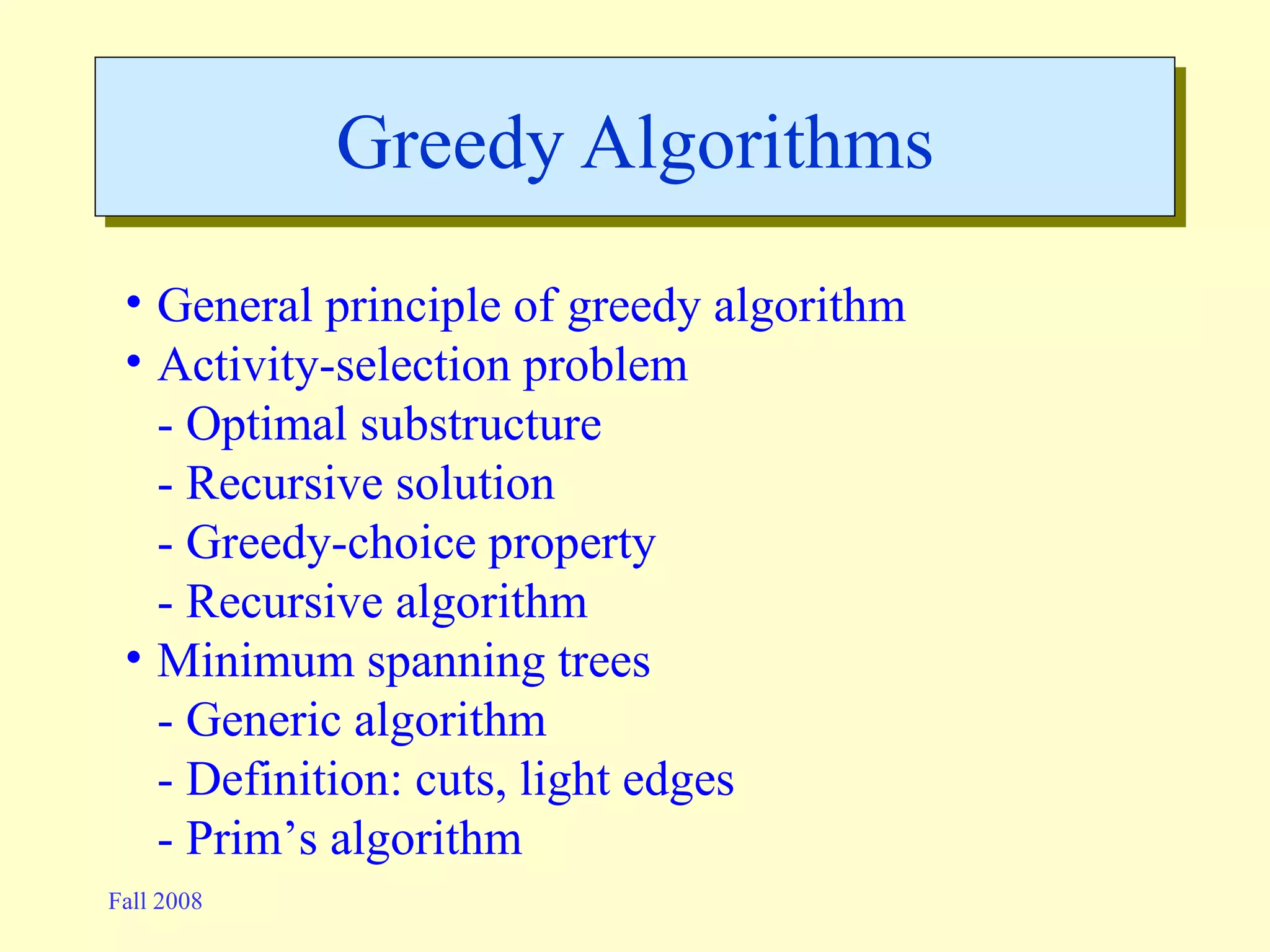
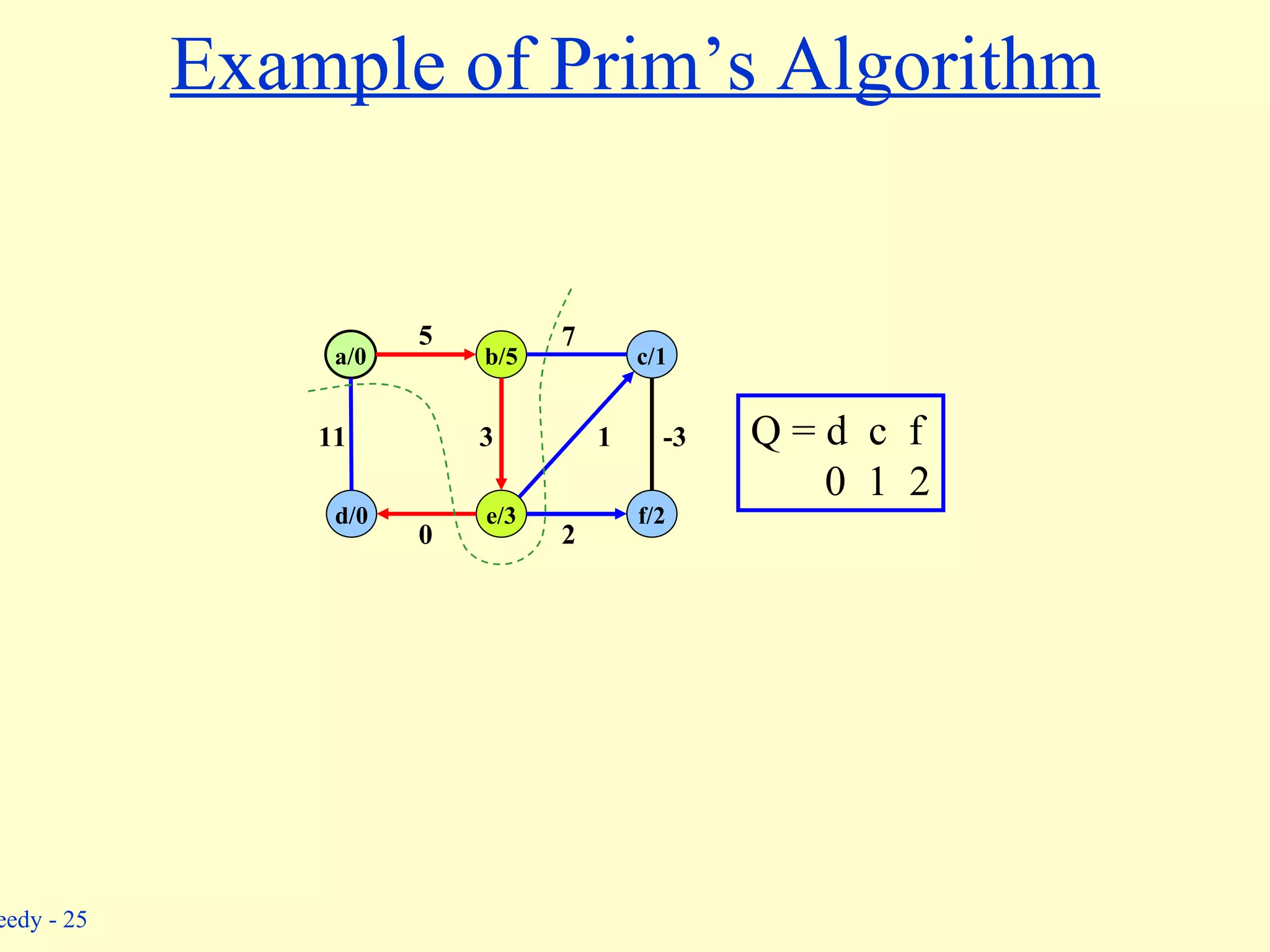
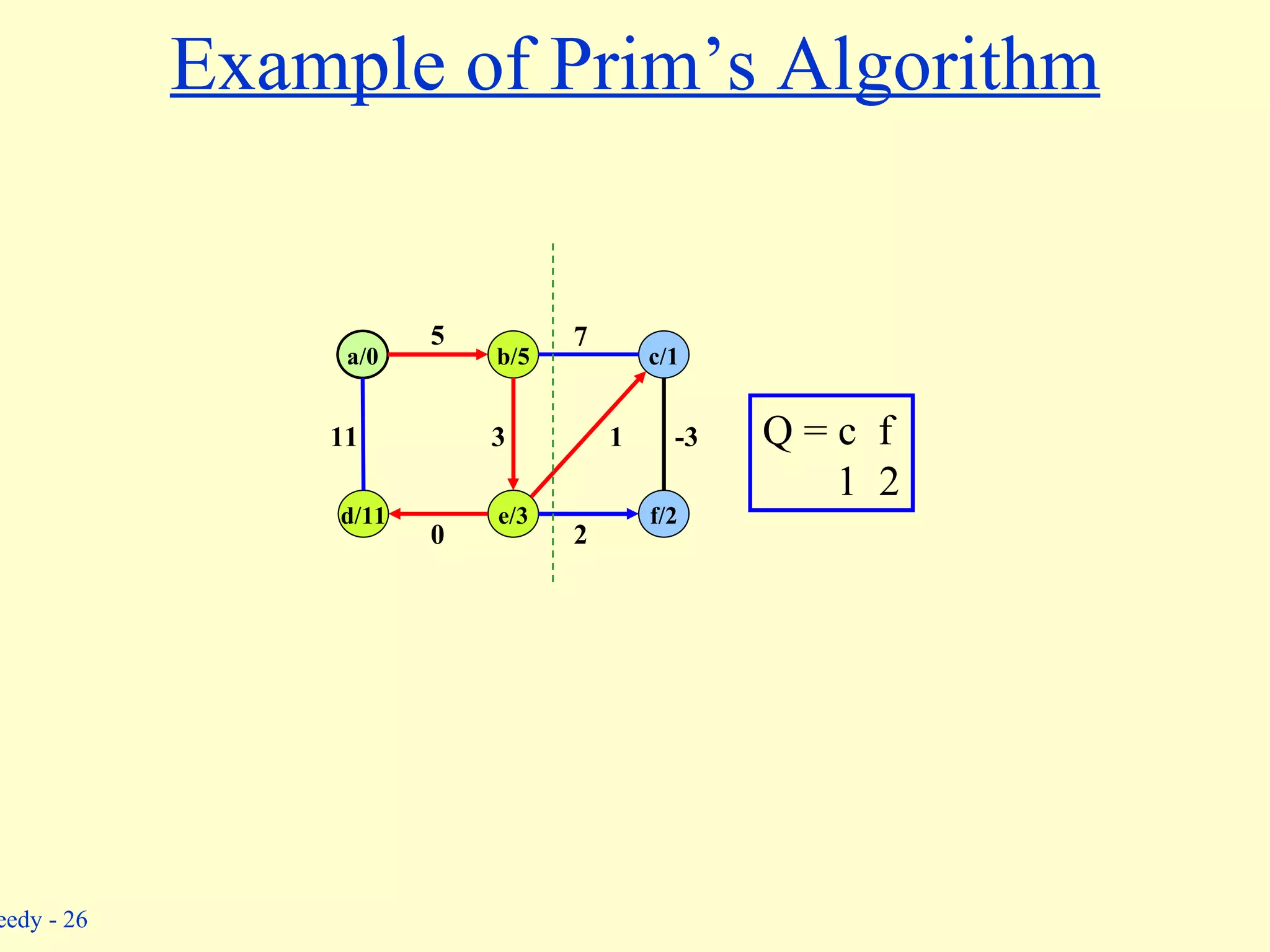
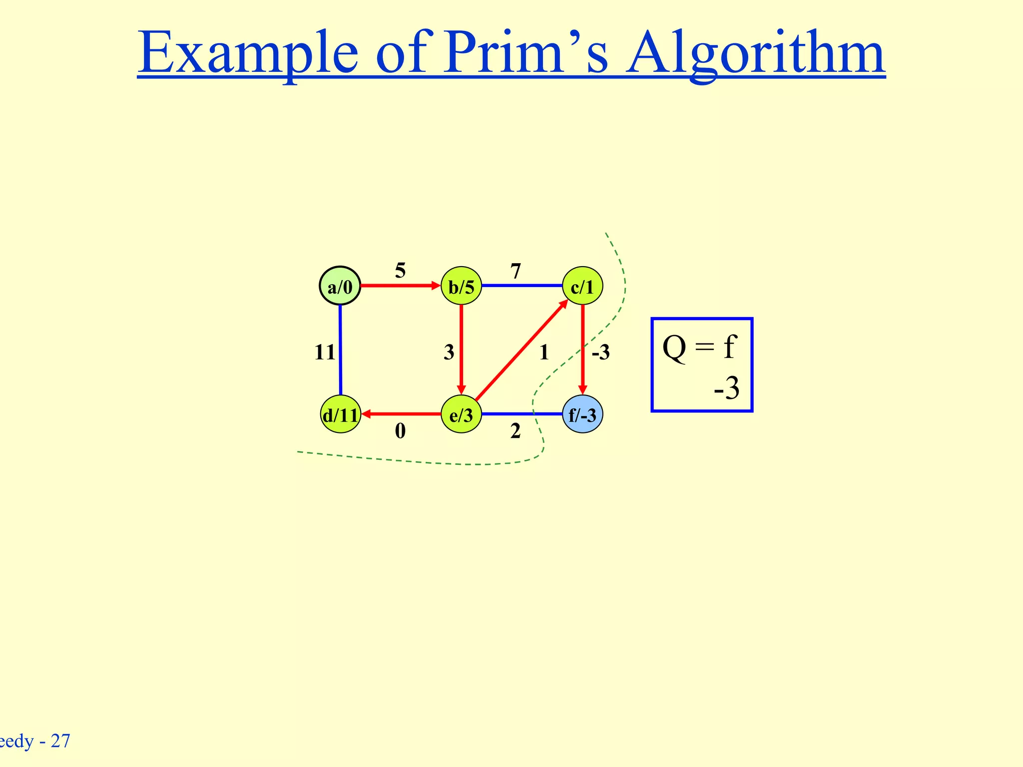
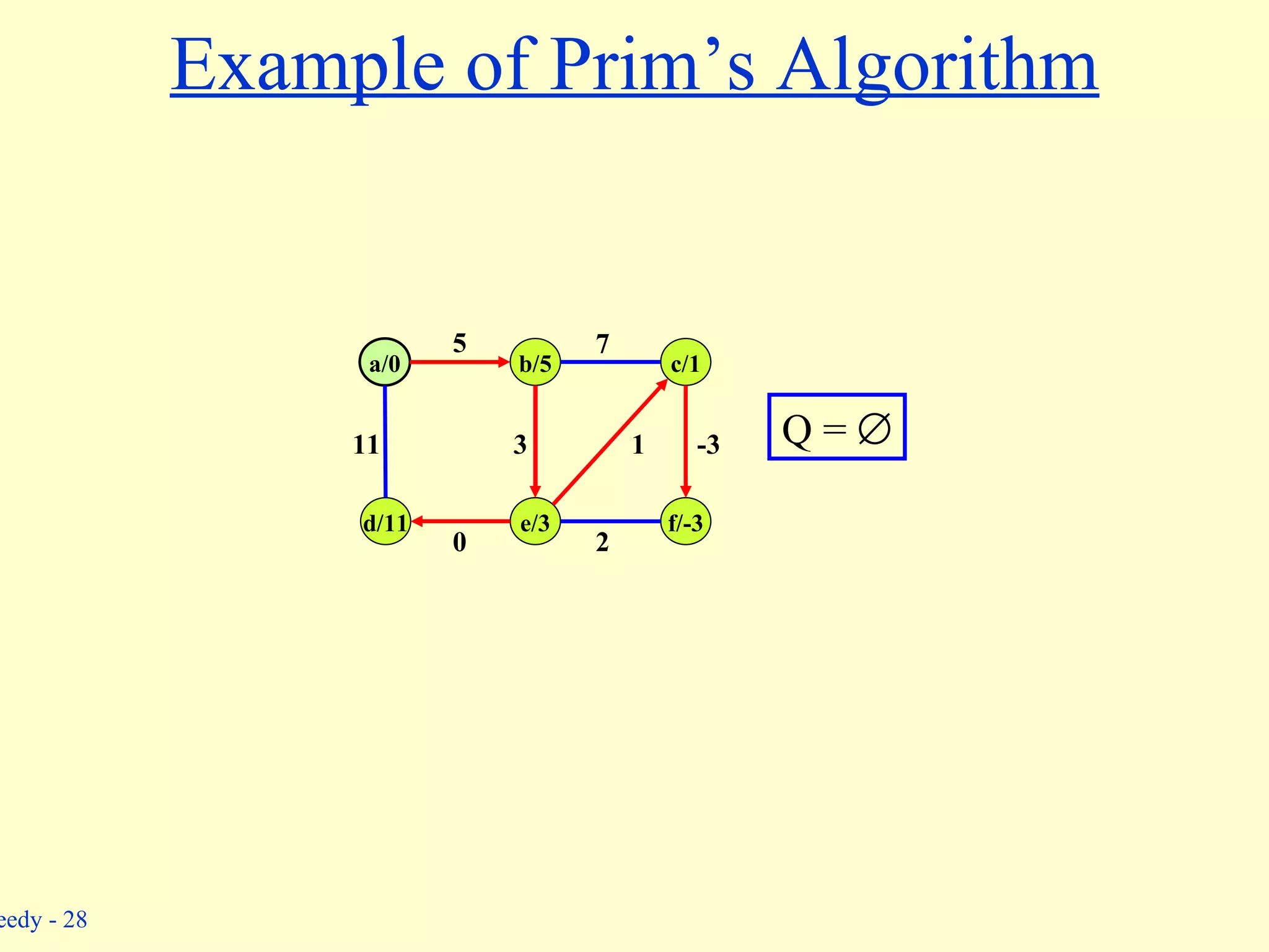
The document discusses greedy algorithms and their properties. It describes how greedy algorithms work by making locally optimal choices at each step in the hope of reaching a globally optimal solution. Two examples are given: the activity selection problem and finding minimum spanning trees. Prim's algorithm for finding minimum spanning trees is described in detail, showing how it works by always selecting the lightest edge between the growing tree and remaining vertices.


![Recursive Solution Let S ij = subset of activities in S that start after a i finishes and finish before a j starts. Subproblems: Selecting maximum number of mutually compatible activities from S ij . Let c [ i , j ] = size of maximum-size subset of mutually compatible activities in S ij . Recursive Solution: ij j k i ij S j k c k i c S j i c if } 1 ] , [ ] , [ max{ if 0 ] , [](https://image.slidesharecdn.com/test-pre805/75/test-pre-7-2048.jpg)


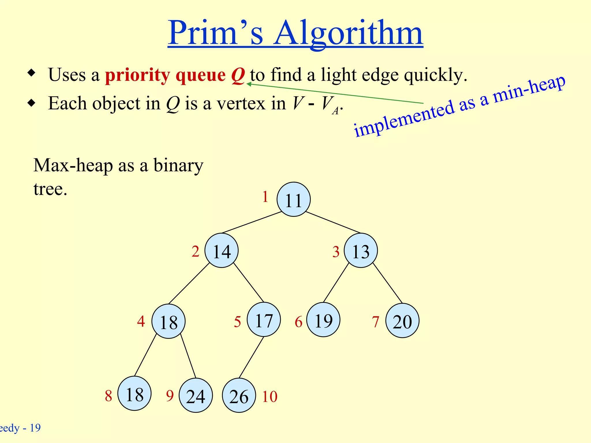
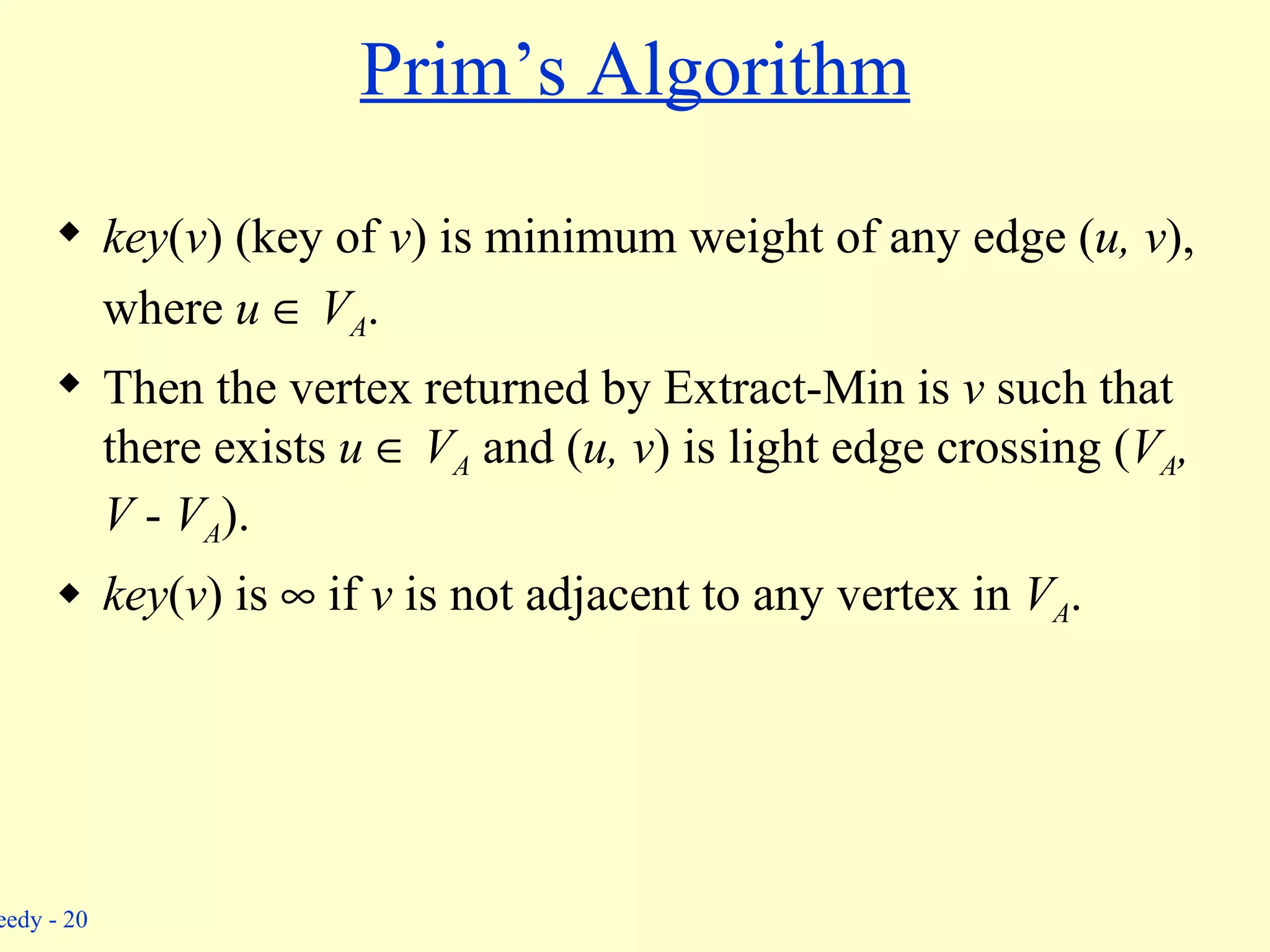
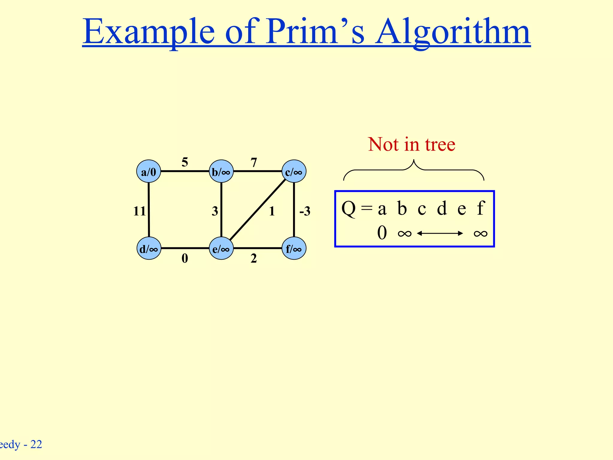
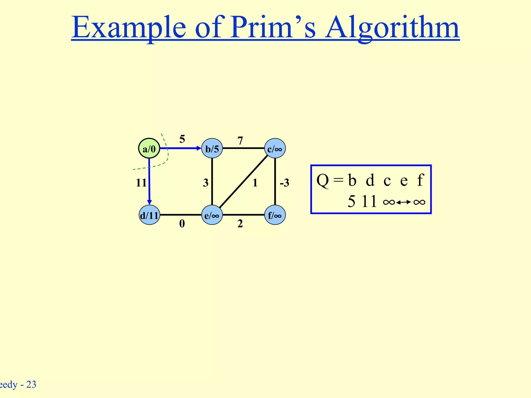
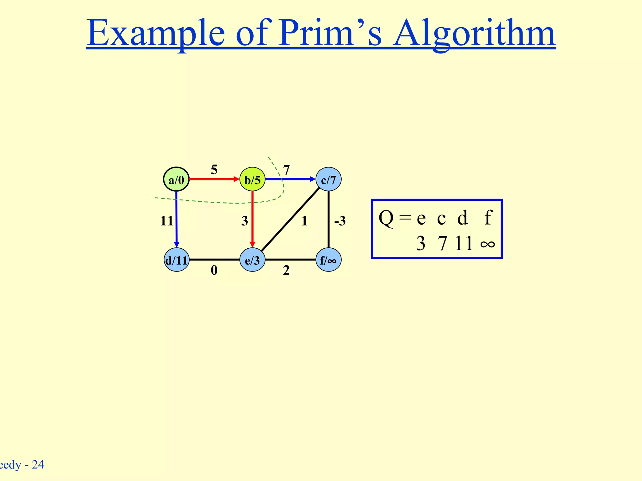
![Prim’s Algorithm Q := V[G]; for each u Q do key[u] := od ; key[r] := 0; [r] := NIL; while Q do u := Extract - Min(Q); for each v Adj[u] do if v Q w(u, v) < key[v] then [v] := u; key[v] := w(u, v) fi od od Complexity: Using binary heaps: O(E lg V). Initialization – O(V). Building initial queue – O(V). V Extract-Min’s – O(V lgV). E Decrease-Key’s – O(E lg V). Using Fibonacci heaps: O(E + V lg V). (see book) Note: A = {(v, [v]) : v v - {r} - Q}. decrease-key operation](https://image.slidesharecdn.com/test-pre805/75/test-pre-21-2048.jpg)


![Recursive Solution Let S ij = subset of activities in S that start after a i finishes and finish before a j starts. Subproblems: Selecting maximum number of mutually compatible activities from S ij . Let c [ i , j ] = size of maximum-size subset of mutually compatible activities in S ij . Recursive Solution: ij j k i ij S j k c k i c S j i c if } 1 ] , [ ] , [ max{ if 0 ] , [](https://crownmelresort.com/image.slidesharecdn.com/test-pre805/75/test-pre-7-2048.jpg)


![Prim’s Algorithm Q := V[G]; for each u Q do key[u] := od ; key[r] := 0; [r] := NIL; while Q do u := Extract - Min(Q); for each v Adj[u] do if v Q w(u, v) < key[v] then [v] := u; key[v] := w(u, v) fi od od Complexity: Using binary heaps: O(E lg V). Initialization – O(V). Building initial queue – O(V). V Extract-Min’s – O(V lgV). E Decrease-Key’s – O(E lg V). Using Fibonacci heaps: O(E + V lg V). (see book) Note: A = {(v, [v]) : v v - {r} - Q}. decrease-key operation](https://crownmelresort.com/image.slidesharecdn.com/test-pre805/75/test-pre-21-2048.jpg)