This document provides a summary of key concepts in artificial intelligence, organized into the following sections:
1. Reflex-based models such as linear predictors for classification and regression using techniques like loss minimization and regularization.
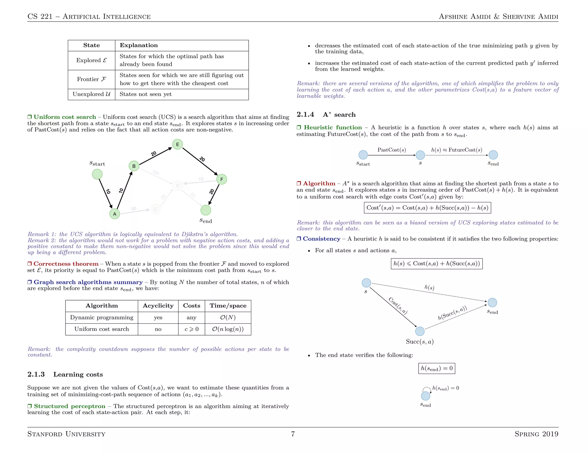
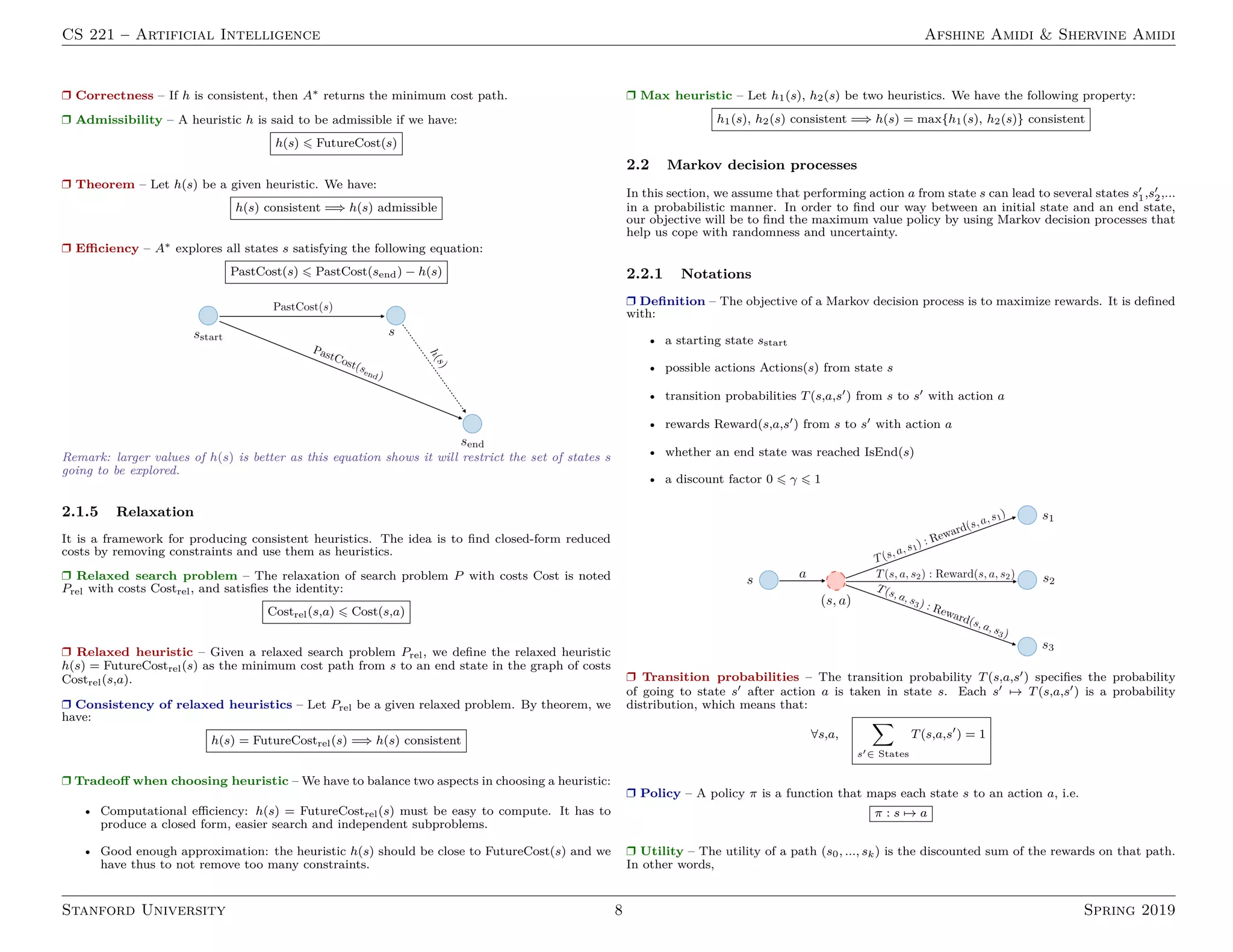
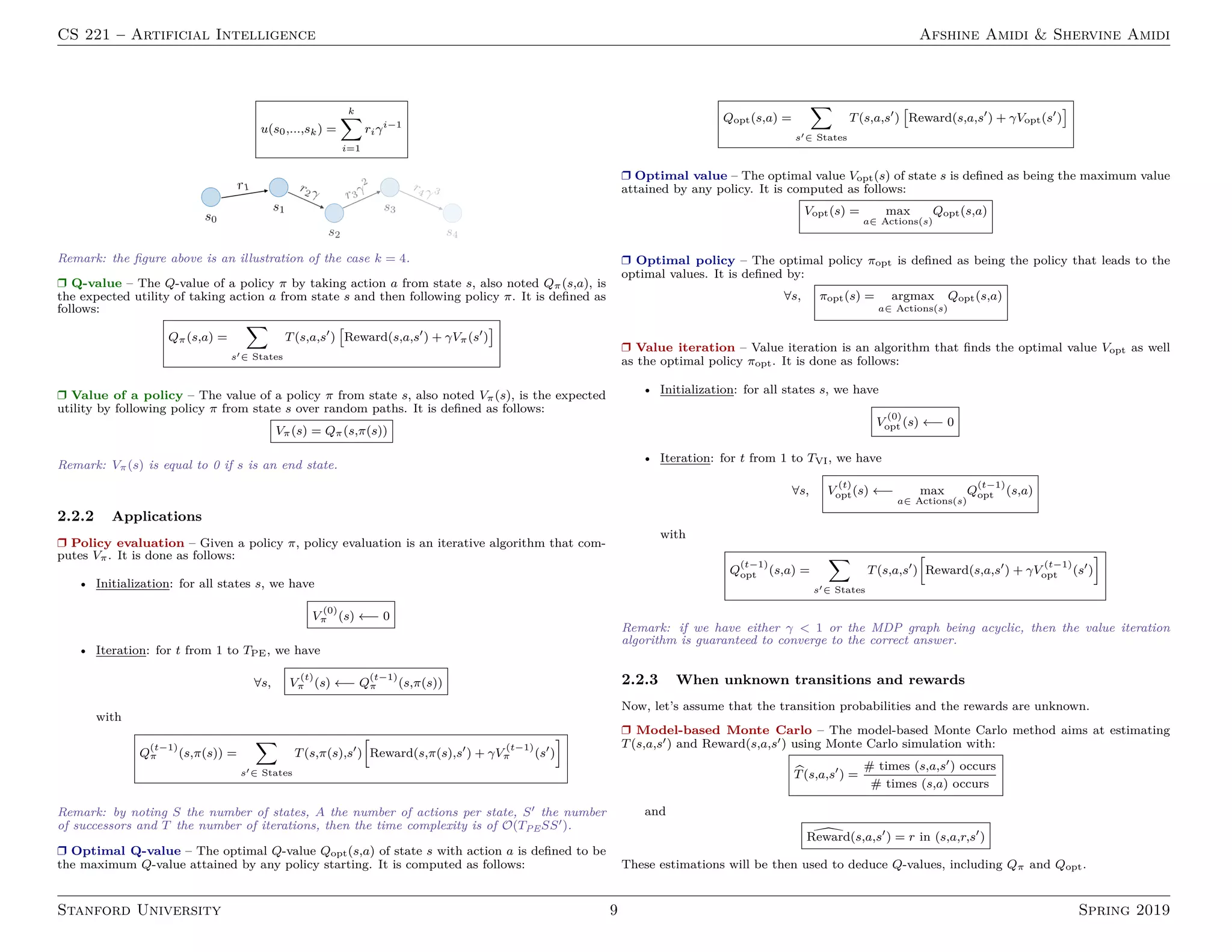
2. States-based models including search optimization techniques like tree search, graph search, A* search and Markov decision processes.
3. Variables-based models covering constraint satisfaction problems, Bayesian networks and inference.
4. Logic-based models discussing knowledge bases, propositional logic and first-order logic.
The document defines important terms and algorithms at a high level across different areas of AI like supervised and unsupervised learning, neural networks, optimization, probabilistic modeling and logic.
![CS 221 – Artificial Intelligence Afshine Amidi Shervine Amidi
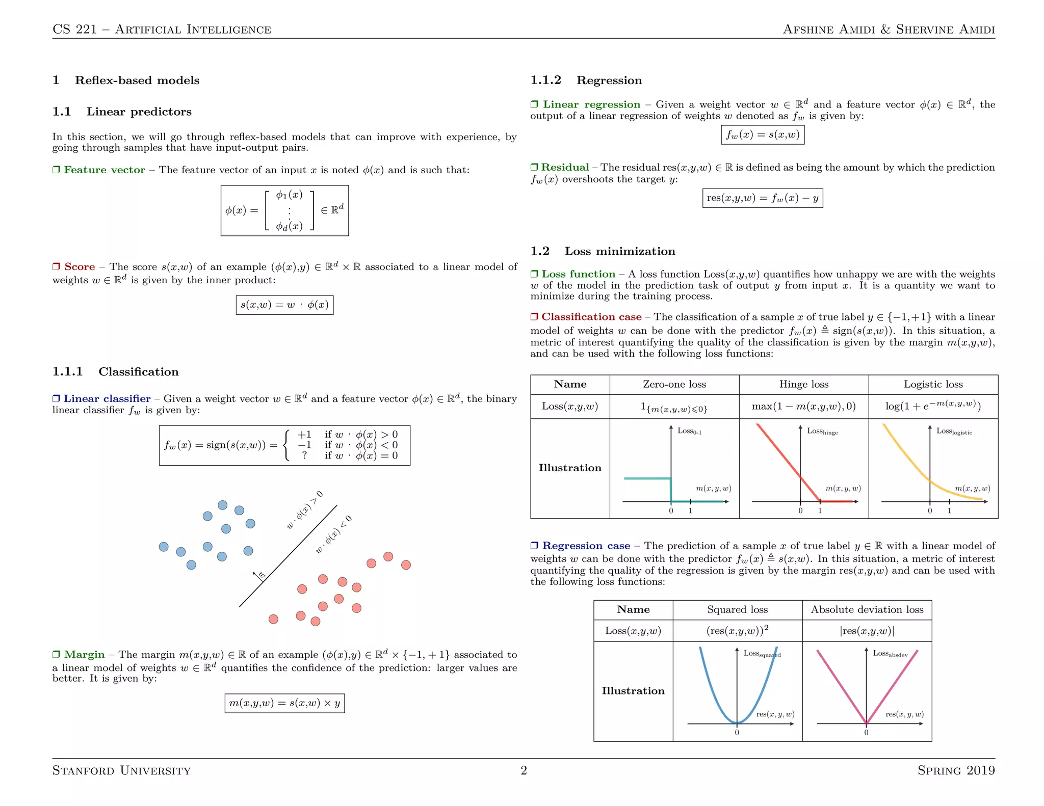
r Loss minimization framework – In order to train a model, we want to minimize the
training loss is defined as follows:
TrainLoss(w) =
1
|Dtrain|
X
(x,y)∈Dtrain
Loss(x,y,w)
1.3 Non-linear predictors
r k-nearest neighbors – The k-nearest neighbors algorithm, commonly known as k-NN, is a
non-parametric approach where the response of a data point is determined by the nature of its
k neighbors from the training set. It can be used in both classification and regression settings.
Remark: the higher the parameter k, the higher the bias, and the lower the parameter k, the
higher the variance.
r Neural networks – Neural networks are a class of models that are built with layers. Com-
monly used types of neural networks include convolutional and recurrent neural networks. The
vocabulary around neural networks architectures is described in the figure below:
By noting i the ith layer of the network and j the jth hidden unit of the layer, we have:
z
[i]
j = w
[i]
j
T
x + b
[i]
j
where we note w, b, x, z the weight, bias, input and non-activated output of the neuron respec-
tively.
1.4 Stochastic gradient descent
r Gradient descent – By noting η ∈ R the learning rate (also called step size), the update
rule for gradient descent is expressed with the learning rate and the loss function Loss(x,y,w) as
follows:
w ←− w − η∇wLoss(x,y,w)
r Stochastic updates – Stochastic gradient descent (SGD) updates the parameters of the
model one training example (φ(x),y) ∈ Dtrain at a time. This method leads to sometimes noisy,
but fast updates.
r Batch updates – Batch gradient descent (BGD) updates the parameters of the model one
batch of examples (e.g. the entire training set) at a time. This method computes stable update
directions, at a greater computational cost.
1.5 Fine-tuning models
r Hypothesis class – A hypothesis class F is the set of possible predictors with a fixed φ(x)
and varying w:
F =
fw : w ∈ Rd
r Logistic function – The logistic function σ, also called the sigmoid function, is defined as:
∀z ∈] − ∞, + ∞[, σ(z) =
1
1 + e−z
Remark: we have σ0(z) = σ(z)(1 − σ(z)).
r Backpropagation – The forward pass is done through fi, which is the value for the subex-
pression rooted at i, while the backward pass is done through gi = ∂out
∂fi
and represents how fi
influences the output.
r Approximation and estimation error – The approximation error approx represents how
far the entire hypothesis class F is from the target predictor g∗, while the estimation error est
quantifies how good the predictor ˆ
f is with respect to the best predictor f∗ of the hypothesis
class F.
Stanford University 3 Spring 2019](https://image.slidesharecdn.com/super-cheatsheet-artificial-intelligence-230419070502-23ad4c9f/75/super-cheatsheet-artificial-intelligence-pdf-3-2048.jpg)
![CS 221 – Artificial Intelligence Afshine Amidi Shervine Amidi
r Regularization – The regularization procedure aims at avoiding the model to overfit the
data and thus deals with high variance issues. The following table sums up the different types
of commonly used regularization techniques:
LASSO Ridge Elastic Net
- Shrinks coefficients to 0
- Good for variable selection
Makes coefficients smaller
Tradeoff between variable
selection and small coefficients
... + λ||θ||1 ... + λ||θ||2
2 ... + λ
h
(1 − α)||θ||1 + α||θ||2
2
i
λ ∈ R λ ∈ R λ ∈ R, α ∈ [0,1]
r Hyperparameters – Hyperparameters are the properties of the learning algorithm, and
include features, regularization parameter λ, number of iterations T, step size η, etc.
r Sets vocabulary – When selecting a model, we distinguish 3 different parts of the data that
we have as follows:
Training set Validation set Testing set
- Model is trained
- Usually 80 of the dataset
- Model is assessed
- Usually 20 of the dataset
- Also called hold-out
- Model gives predictions
- Unseen data
or development set
Once the model has been chosen, it is trained on the entire dataset and tested on the unseen
test set. These are represented in the figure below:
1.6 Unsupervised Learning
The class of unsupervised learning methods aims at discovering the structure of the data, which
may have of rich latent structures.
1.6.1 k-means
r Clustering – Given a training set of input points Dtrain, the goal of a clustering algorithm
is to assign each point φ(xi) to a cluster zi ∈ {1,...,k}.
r Objective function – The loss function for one of the main clustering algorithms, k-means,
is given by:
Lossk-means(x,µ) =
n
X
i=1
||φ(xi) − µzi ||2
r Algorithm – After randomly initializing the cluster centroids µ1,µ2,...,µk ∈ Rn, the k-means
algorithm repeats the following step until convergence:
zi = arg min
j
||φ(xi) − µj||2
and µj =
m
X
i=1
1{zi=j}φ(xi)
m
X
i=1
1{zi=j}
1.6.2 Principal Component Analysis
r Eigenvalue, eigenvector – Given a matrix A ∈ Rn×n, λ is said to be an eigenvalue of A if
there exists a vector z ∈ Rn{0}, called eigenvector, such that we have:
Az = λz
Stanford University 4 Spring 2019](https://image.slidesharecdn.com/super-cheatsheet-artificial-intelligence-230419070502-23ad4c9f/75/super-cheatsheet-artificial-intelligence-pdf-4-2048.jpg)
![CS 221 – Artificial Intelligence Afshine Amidi Shervine Amidi
Remark: model-based Monte Carlo is said to be off-policy, because the estimation does not
depend on the exact policy.
r Model-free Monte Carlo – The model-free Monte Carlo method aims at directly estimating
Qπ, as follows:
b
Qπ(s,a) = average of ut where st−1 = s, at = a
where ut denotes the utility starting at step t of a given episode.
Remark: model-free Monte Carlo is said to be on-policy, because the estimated value is dependent
on the policy π used to generate the data.
r Equivalent formulation – By introducing the constant η = 1
1+(#updates to (s,a))
and for
each (s,a,u) of the training set, the update rule of model-free Monte Carlo has a convex combi-
nation formulation:
b
Qπ(s,a) ← (1 − η) b
Qπ(s,a) + ηu
as well as a stochastic gradient formulation:
b
Qπ(s,a) ← b
Qπ(s,a) − η( b
Qπ(s,a) − u)
r SARSA – State-action-reward-state-action (SARSA) is a boostrapping method estimating
Qπ by using both raw data and estimates as part of the update rule. For each (s,a,r,s0,a0), we
have:
b
Qπ(s,a) ←− (1 − η) b
Qπ(s,a) + η
h
r + γ b
Qπ(s0
,a0
)
i
Remark: the SARSA estimate is updated on the fly as opposed to the model-free Monte Carlo
one where the estimate can only be updated at the end of the episode.
r Q-learning – Q-learning is an off-policy algorithm that produces an estimate for Qopt. On
each (s,a,r,s0,a0), we have:
b
Qopt(s,a) ← (1 − η) b
Qopt(s,a) + η
h
r + γ max
a0∈ Actions(s0)
b
Qopt(s0
,a0
)
i
r Epsilon-greedy – The epsilon-greedy policy is an algorithm that balances exploration with
probability and exploitation with probability 1 − . For a given state s, the policy πact is
computed as follows:
πact(s) =
argmax
a∈ Actions
b
Qopt(s,a) with proba 1 −
random from Actions(s) with proba
2.3 Game playing
In games (e.g. chess, backgammon, Go), other agents are present and need to be taken into
account when constructing our policy.
r Game tree – A game tree is a tree that describes the possibilities of a game. In particular,
each node is a decision point for a player and each root-to-leaf path is a possible outcome of the
game.
r Two-player zero-sum game – It is a game where each state is fully observed and such that
players take turns. It is defined with:
• a starting state sstart
• possible actions Actions(s) from state s
• successors Succ(s,a) from states s with actions a
• whether an end state was reached IsEnd(s)
• the agent’s utility Utility(s) at end state s
• the player Player(s) who controls state s
Remark: we will assume that the utility of the agent has the opposite sign of the one of the
opponent.
r Types of policies – There are two types of policies:
• Deterministic policies, noted πp(s), which are actions that player p takes in state s.
• Stochastic policies, noted πp(s,a) ∈ [0,1], which are probabilities that player p takes action
a in state s.
r Expectimax – For a given state s, the expectimax value Vexptmax(s) is the maximum expected
utility of any agent policy when playing with respect to a fixed and known opponent policy πopp.
It is computed as follows:
Vexptmax(s) =
Utility(s) IsEnd(s)
max
a∈Actions(s)
Vexptmax(Succ(s,a)) Player(s) = agent
X
a∈Actions(s)
πopp(s,a)Vexptmax(Succ(s,a)) Player(s) = opp
Remark: expectimax is the analog of value iteration for MDPs.
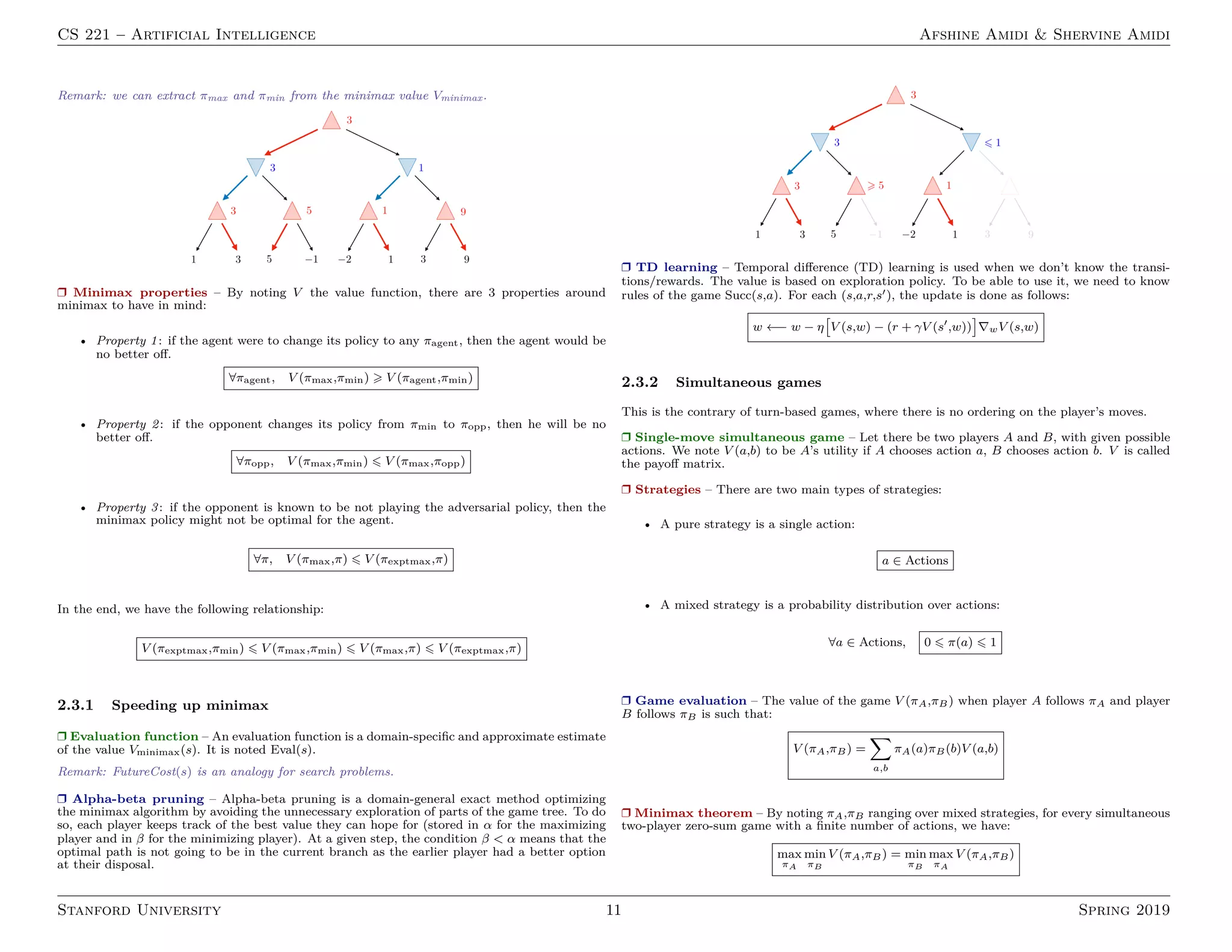
r Minimax – The goal of minimax policies is to find an optimal policy against an adversary
by assuming the worst case, i.e. that the opponent is doing everything to minimize the agent’s
utility. It is done as follows:
Vminimax(s) =
Utility(s) IsEnd(s)
max
a∈Actions(s)
Vminimax(Succ(s,a)) Player(s) = agent
min
a∈Actions(s)
Vminimax(Succ(s,a)) Player(s) = opp
Stanford University 10 Spring 2019](https://image.slidesharecdn.com/super-cheatsheet-artificial-intelligence-230419070502-23ad4c9f/75/super-cheatsheet-artificial-intelligence-pdf-10-2048.jpg)
![CS 221 – Artificial Intelligence Afshine Amidi Shervine Amidi
2.3.3 Non-zero-sum games
r Payoff matrix – We define Vp(πA,πB) to be the utility for player p.
r Nash equilibrium – A Nash equilibrium is (π∗
A,π∗
B) such that no player has an incentive to
change its strategy. We have:
∀πA, VA(π∗
A,π∗
B) VA(πA,π∗
B) and ∀πB, VB(π∗
A,π∗
B) VB(π∗
A,πB)
Remark: in any finite-player game with finite number of actions, there exists at least one Nash
equilibrium.
3 Variables-based models
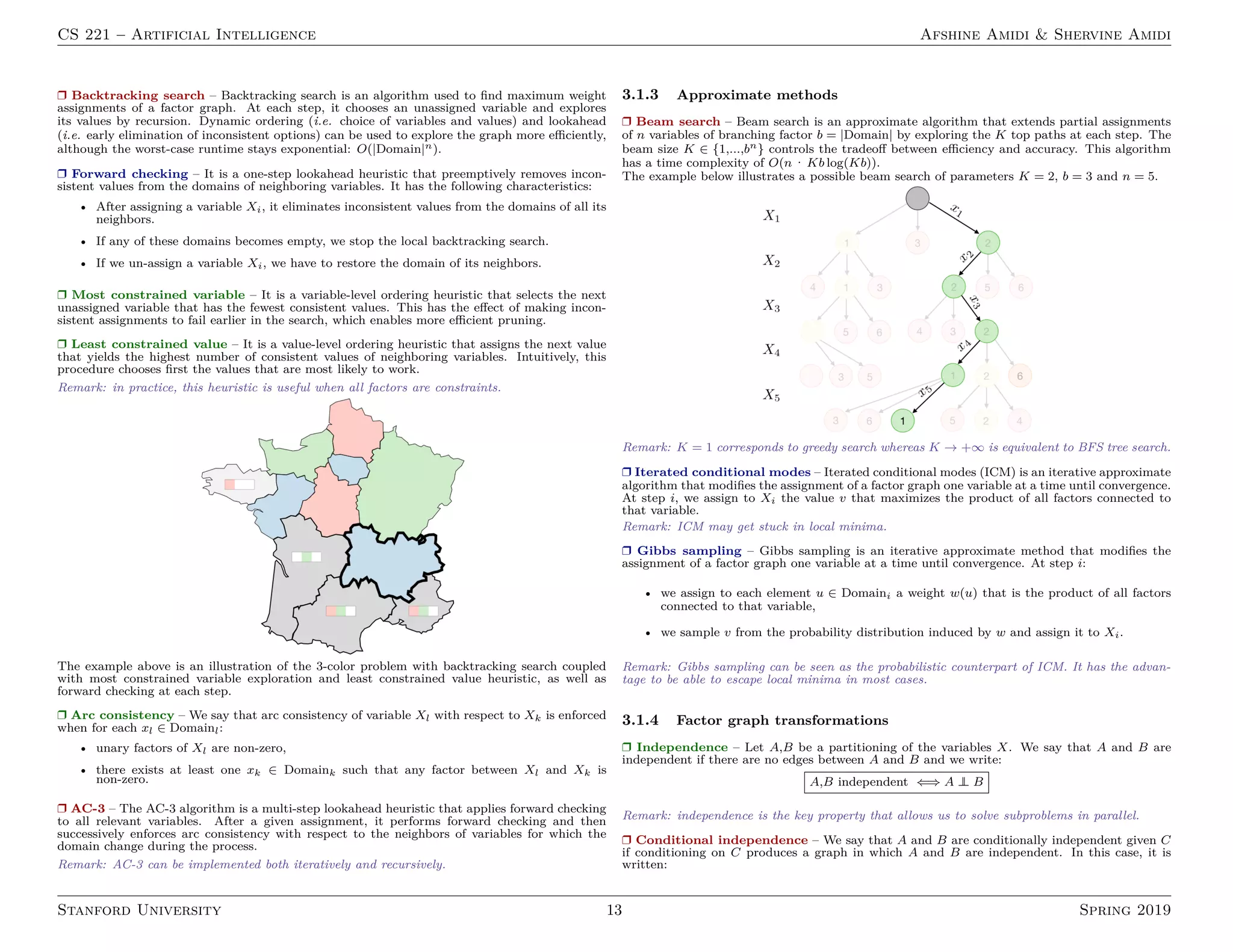
3.1 Constraint satisfaction problems
In this section, our objective is to find maximum weight assignments of variable-based models.
One advantage compared to states-based models is that these algorithms are more convenient
to encode problem-specific constraints.
3.1.1 Factor graphs
r Definition – A factor graph, also referred to as a Markov random field, is a set of variables
X = (X1,...,Xn) where Xi ∈ Domaini and m factors f1,...,fm with each fj(X) 0.
r Scope and arity – The scope of a factor fj is the set of variables it depends on. The size of
this set is called the arity.
Remark: factors of arity 1 and 2 are called unary and binary respectively.
r Assignment weight – Each assignment x = (x1,...,xn) yields a weight Weight(x) defined as
being the product of all factors fj applied to that assignment. Its expression is given by:
Weight(x) =
m
Y
j=1
fj(x)
r Constraint satisfaction problem – A constraint satisfaction problem (CSP) is a factor
graph where all factors are binary; we call them to be constraints:
∀j ∈ [[1,m]], fj(x) ∈ {0,1}
Here, the constraint j with assignment x is said to be satisfied if and only if fj(x) = 1.
r Consistent assignment – An assignment x of a CSP is said to be consistent if and only if
Weight(x) = 1, i.e. all constraints are satisfied.
3.1.2 Dynamic ordering
r Dependent factors – The set of dependent factors of variable Xi with partial assignment x
is called D(x,Xi), and denotes the set of factors that link Xi to already assigned variables.
Stanford University 12 Spring 2019](https://image.slidesharecdn.com/super-cheatsheet-artificial-intelligence-230419070502-23ad4c9f/75/super-cheatsheet-artificial-intelligence-pdf-12-2048.jpg)

![CS 221 – Artificial Intelligence Afshine Amidi Shervine Amidi
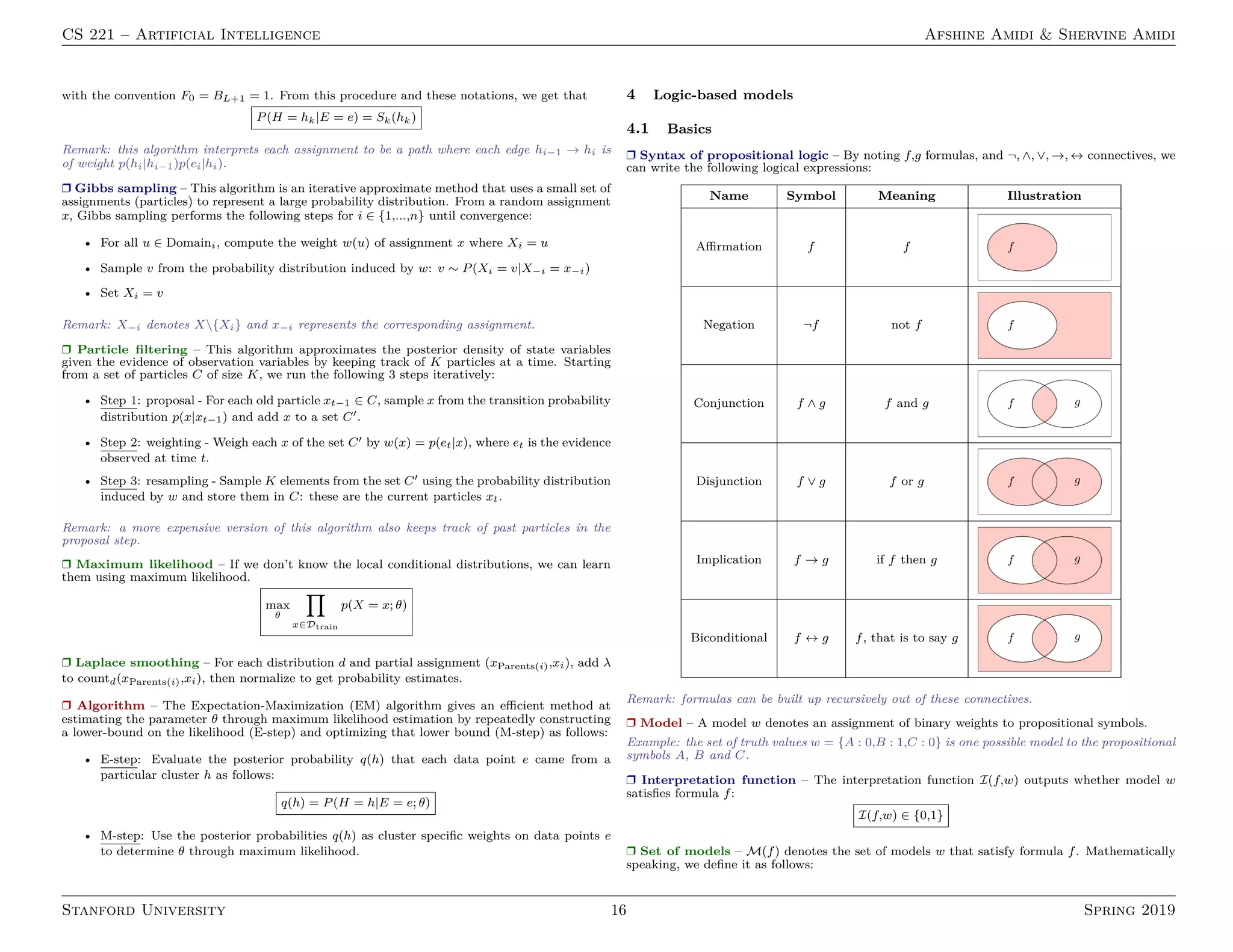
4.3 Propositional logic
In this section, we will go through logic-based models that use logical formulas and inference
rules. The idea here is to balance expressivity and computational efficiency.
r Horn clause – By noting p1,...,pk and q propositional symbols, a Horn clause has the form:
(p1 ∧ ... ∧ pk) −→ q
Remark: when q = false, it is called a goal clause, otherwise we denote it as a definite
clause.
r Modus ponens inference rule – For propositional symbols f1,...,fk and p, the modus
ponens rule is written:
f1,...,fk, (f1 ∧ ... ∧ fk) −→ p
p
Remark: it takes linear time to apply this rule, as each application generate a clause that
contains a single propositional symbol.
r Completeness – Modus ponens is complete with respect to Horn clauses if we suppose that
KB contains only Horn clauses and p is an entailed propositional symbol. Applying modus
ponens will then derive p.
r Conjunctive normal form – A conjunctive normal form (CNF) formula is a conjunction of
clauses, where each clause is a disjunction of atomic formulas.
Remark: in other words, CNFs are ∧ of ∨.
r Equivalent representation – Every formula in propositional logic can be written into an
equivalent CNF formula. The table below presents general conversion properties:
Rule name Initial Converted
Eliminate
↔ f ↔ g (f → g) ∧ (g → f)
→ f → g ¬f ∨ g
¬¬ ¬¬f f
Distribute
¬ over ∧ ¬(f ∧ g) ¬f ∨ ¬g
¬ over ∨ ¬(f ∨ g) ¬f ∧ ¬g
∨ over ∧ f ∨ (g ∧ h) (f ∨ g) ∧ (f ∨ h)
r Resolution inference rule – For propositional symbols f1,...,fn, and g1,...,gm as well as p,
the resolution rule is written:
f1 ∨ ... ∨ fn ∨ p, ¬p ∨ g1 ∨ ... ∨ gm
f1 ∨ ... ∨ fn ∨ g1 ∨ ... ∨ gm
Remark: it can take exponential time to apply this rule, as each application generates a clause
that has a subset of the propositional symbols.
r Resolution-based inference – The resolution-based inference algorithm follows the follow-
ing steps:
• Step 1: Convert all formulas into CNF
• Step 2: Repeatedly apply resolution rule
• Step 3: Return unsatisfiable if and only if False is derived
4.4 First-order logic
The idea here is that variables yield compact knowledge representations.
r Model – A model w in first-order logic maps:
• constant symbols to objects
• predicate symbols to tuple of objects
r Horn clause – By noting x1,...,xn variables and a1,...,ak,b atomic formulas, the first-order
logic version of a horn clause has the form:
∀x1,...,∀xn, (a1 ∧ ... ∧ ak) → b
r Substitution – A substitution θ maps variables to terms and Subst(θ,f) denotes the result
of substitution θ on f.
r Unification – Unification takes two formulas f and g and returns the most general substitu-
tion θ that makes them equal:
Unify[f,g] = θ s.t. Subst[θ,f] = Subst[θ,g]
Note: Unify[f,g] returns Fail if no such θ exists.
r Modus ponens – By noting x1,...,xn variables, a1,...,ak and a0
1,...,a0
k atomic formulas and
by calling θ = Unify(a0
1 ∧ ... ∧ a0
k, a1 ∧ ... ∧ ak) the first-order logic version of modus ponens can
be written:
a0
1,...,a0
k ∀x1,...,∀xn(a1 ∧ ... ∧ ak) → b
Subst[θ, b]
r Completeness – Modus ponens is complete for first-order logic with only Horn clauses.
r Resolution rule – By noting f1, ..., fn, g1, ..., gm, p, q formulas and by calling θ = Unify(p,q),
the first-order logic version of the resolution rule can be written:
f1 ∨ ... ∨ fn ∨ p, ¬q ∨ g1 ∨ ... ∨ gm
Subst[θ,f1 ∨ ... ∨ fn ∨ g1 ∨ ... ∨ gm]
r Semi-decidability – First-order logic, even restricted to only Horn clauses, is semi-decidable.
• if KB |= f, forward inference on complete inference rules will prove f in finite time
• if KB 6|= f, no algorithm can show this in finite time
Stanford University 18 Spring 2019](https://image.slidesharecdn.com/super-cheatsheet-artificial-intelligence-230419070502-23ad4c9f/75/super-cheatsheet-artificial-intelligence-pdf-18-2048.jpg)


![CS 221 – Artificial Intelligence Afshine Amidi Shervine Amidi
r Loss minimization framework – In order to train a model, we want to minimize the
training loss is defined as follows:
TrainLoss(w) =
1
|Dtrain|
X
(x,y)∈Dtrain
Loss(x,y,w)
1.3 Non-linear predictors
r k-nearest neighbors – The k-nearest neighbors algorithm, commonly known as k-NN, is a
non-parametric approach where the response of a data point is determined by the nature of its
k neighbors from the training set. It can be used in both classification and regression settings.
Remark: the higher the parameter k, the higher the bias, and the lower the parameter k, the
higher the variance.
r Neural networks – Neural networks are a class of models that are built with layers. Com-
monly used types of neural networks include convolutional and recurrent neural networks. The
vocabulary around neural networks architectures is described in the figure below:
By noting i the ith layer of the network and j the jth hidden unit of the layer, we have:
z
[i]
j = w
[i]
j
T
x + b
[i]
j
where we note w, b, x, z the weight, bias, input and non-activated output of the neuron respec-
tively.
1.4 Stochastic gradient descent
r Gradient descent – By noting η ∈ R the learning rate (also called step size), the update
rule for gradient descent is expressed with the learning rate and the loss function Loss(x,y,w) as
follows:
w ←− w − η∇wLoss(x,y,w)
r Stochastic updates – Stochastic gradient descent (SGD) updates the parameters of the
model one training example (φ(x),y) ∈ Dtrain at a time. This method leads to sometimes noisy,
but fast updates.
r Batch updates – Batch gradient descent (BGD) updates the parameters of the model one
batch of examples (e.g. the entire training set) at a time. This method computes stable update
directions, at a greater computational cost.
1.5 Fine-tuning models
r Hypothesis class – A hypothesis class F is the set of possible predictors with a fixed φ(x)
and varying w:
F =
fw : w ∈ Rd
r Logistic function – The logistic function σ, also called the sigmoid function, is defined as:
∀z ∈] − ∞, + ∞[, σ(z) =
1
1 + e−z
Remark: we have σ0(z) = σ(z)(1 − σ(z)).
r Backpropagation – The forward pass is done through fi, which is the value for the subex-
pression rooted at i, while the backward pass is done through gi = ∂out
∂fi
and represents how fi
influences the output.
r Approximation and estimation error – The approximation error approx represents how
far the entire hypothesis class F is from the target predictor g∗, while the estimation error est
quantifies how good the predictor ˆ
f is with respect to the best predictor f∗ of the hypothesis
class F.
Stanford University 3 Spring 2019](https://crownmelresort.com/image.slidesharecdn.com/super-cheatsheet-artificial-intelligence-230419070502-23ad4c9f/75/super-cheatsheet-artificial-intelligence-pdf-3-2048.jpg)
![CS 221 – Artificial Intelligence Afshine Amidi Shervine Amidi
r Regularization – The regularization procedure aims at avoiding the model to overfit the
data and thus deals with high variance issues. The following table sums up the different types
of commonly used regularization techniques:
LASSO Ridge Elastic Net
- Shrinks coefficients to 0
- Good for variable selection
Makes coefficients smaller
Tradeoff between variable
selection and small coefficients
... + λ||θ||1 ... + λ||θ||2
2 ... + λ
h
(1 − α)||θ||1 + α||θ||2
2
i
λ ∈ R λ ∈ R λ ∈ R, α ∈ [0,1]
r Hyperparameters – Hyperparameters are the properties of the learning algorithm, and
include features, regularization parameter λ, number of iterations T, step size η, etc.
r Sets vocabulary – When selecting a model, we distinguish 3 different parts of the data that
we have as follows:
Training set Validation set Testing set
- Model is trained
- Usually 80 of the dataset
- Model is assessed
- Usually 20 of the dataset
- Also called hold-out
- Model gives predictions
- Unseen data
or development set
Once the model has been chosen, it is trained on the entire dataset and tested on the unseen
test set. These are represented in the figure below:
1.6 Unsupervised Learning
The class of unsupervised learning methods aims at discovering the structure of the data, which
may have of rich latent structures.
1.6.1 k-means
r Clustering – Given a training set of input points Dtrain, the goal of a clustering algorithm
is to assign each point φ(xi) to a cluster zi ∈ {1,...,k}.
r Objective function – The loss function for one of the main clustering algorithms, k-means,
is given by:
Lossk-means(x,µ) =
n
X
i=1
||φ(xi) − µzi ||2
r Algorithm – After randomly initializing the cluster centroids µ1,µ2,...,µk ∈ Rn, the k-means
algorithm repeats the following step until convergence:
zi = arg min
j
||φ(xi) − µj||2
and µj =
m
X
i=1
1{zi=j}φ(xi)
m
X
i=1
1{zi=j}
1.6.2 Principal Component Analysis
r Eigenvalue, eigenvector – Given a matrix A ∈ Rn×n, λ is said to be an eigenvalue of A if
there exists a vector z ∈ Rn{0}, called eigenvector, such that we have:
Az = λz
Stanford University 4 Spring 2019](https://crownmelresort.com/image.slidesharecdn.com/super-cheatsheet-artificial-intelligence-230419070502-23ad4c9f/75/super-cheatsheet-artificial-intelligence-pdf-4-2048.jpg)


![CS 221 – Artificial Intelligence Afshine Amidi Shervine Amidi
Remark: model-based Monte Carlo is said to be off-policy, because the estimation does not
depend on the exact policy.
r Model-free Monte Carlo – The model-free Monte Carlo method aims at directly estimating
Qπ, as follows:
b
Qπ(s,a) = average of ut where st−1 = s, at = a
where ut denotes the utility starting at step t of a given episode.
Remark: model-free Monte Carlo is said to be on-policy, because the estimated value is dependent
on the policy π used to generate the data.
r Equivalent formulation – By introducing the constant η = 1
1+(#updates to (s,a))
and for
each (s,a,u) of the training set, the update rule of model-free Monte Carlo has a convex combi-
nation formulation:
b
Qπ(s,a) ← (1 − η) b
Qπ(s,a) + ηu
as well as a stochastic gradient formulation:
b
Qπ(s,a) ← b
Qπ(s,a) − η( b
Qπ(s,a) − u)
r SARSA – State-action-reward-state-action (SARSA) is a boostrapping method estimating
Qπ by using both raw data and estimates as part of the update rule. For each (s,a,r,s0,a0), we
have:
b
Qπ(s,a) ←− (1 − η) b
Qπ(s,a) + η
h
r + γ b
Qπ(s0
,a0
)
i
Remark: the SARSA estimate is updated on the fly as opposed to the model-free Monte Carlo
one where the estimate can only be updated at the end of the episode.
r Q-learning – Q-learning is an off-policy algorithm that produces an estimate for Qopt. On
each (s,a,r,s0,a0), we have:
b
Qopt(s,a) ← (1 − η) b
Qopt(s,a) + η
h
r + γ max
a0∈ Actions(s0)
b
Qopt(s0
,a0
)
i
r Epsilon-greedy – The epsilon-greedy policy is an algorithm that balances exploration with
probability and exploitation with probability 1 − . For a given state s, the policy πact is
computed as follows:
πact(s) =
argmax
a∈ Actions
b
Qopt(s,a) with proba 1 −
random from Actions(s) with proba
2.3 Game playing
In games (e.g. chess, backgammon, Go), other agents are present and need to be taken into
account when constructing our policy.
r Game tree – A game tree is a tree that describes the possibilities of a game. In particular,
each node is a decision point for a player and each root-to-leaf path is a possible outcome of the
game.
r Two-player zero-sum game – It is a game where each state is fully observed and such that
players take turns. It is defined with:
• a starting state sstart
• possible actions Actions(s) from state s
• successors Succ(s,a) from states s with actions a
• whether an end state was reached IsEnd(s)
• the agent’s utility Utility(s) at end state s
• the player Player(s) who controls state s
Remark: we will assume that the utility of the agent has the opposite sign of the one of the
opponent.
r Types of policies – There are two types of policies:
• Deterministic policies, noted πp(s), which are actions that player p takes in state s.
• Stochastic policies, noted πp(s,a) ∈ [0,1], which are probabilities that player p takes action
a in state s.
r Expectimax – For a given state s, the expectimax value Vexptmax(s) is the maximum expected
utility of any agent policy when playing with respect to a fixed and known opponent policy πopp.
It is computed as follows:
Vexptmax(s) =
Utility(s) IsEnd(s)
max
a∈Actions(s)
Vexptmax(Succ(s,a)) Player(s) = agent
X
a∈Actions(s)
πopp(s,a)Vexptmax(Succ(s,a)) Player(s) = opp
Remark: expectimax is the analog of value iteration for MDPs.
r Minimax – The goal of minimax policies is to find an optimal policy against an adversary
by assuming the worst case, i.e. that the opponent is doing everything to minimize the agent’s
utility. It is done as follows:
Vminimax(s) =
Utility(s) IsEnd(s)
max
a∈Actions(s)
Vminimax(Succ(s,a)) Player(s) = agent
min
a∈Actions(s)
Vminimax(Succ(s,a)) Player(s) = opp
Stanford University 10 Spring 2019](https://crownmelresort.com/image.slidesharecdn.com/super-cheatsheet-artificial-intelligence-230419070502-23ad4c9f/75/super-cheatsheet-artificial-intelligence-pdf-10-2048.jpg)

![CS 221 – Artificial Intelligence Afshine Amidi Shervine Amidi
2.3.3 Non-zero-sum games
r Payoff matrix – We define Vp(πA,πB) to be the utility for player p.
r Nash equilibrium – A Nash equilibrium is (π∗
A,π∗
B) such that no player has an incentive to
change its strategy. We have:
∀πA, VA(π∗
A,π∗
B) VA(πA,π∗
B) and ∀πB, VB(π∗
A,π∗
B) VB(π∗
A,πB)
Remark: in any finite-player game with finite number of actions, there exists at least one Nash
equilibrium.
3 Variables-based models
3.1 Constraint satisfaction problems
In this section, our objective is to find maximum weight assignments of variable-based models.
One advantage compared to states-based models is that these algorithms are more convenient
to encode problem-specific constraints.
3.1.1 Factor graphs
r Definition – A factor graph, also referred to as a Markov random field, is a set of variables
X = (X1,...,Xn) where Xi ∈ Domaini and m factors f1,...,fm with each fj(X) 0.
r Scope and arity – The scope of a factor fj is the set of variables it depends on. The size of
this set is called the arity.
Remark: factors of arity 1 and 2 are called unary and binary respectively.
r Assignment weight – Each assignment x = (x1,...,xn) yields a weight Weight(x) defined as
being the product of all factors fj applied to that assignment. Its expression is given by:
Weight(x) =
m
Y
j=1
fj(x)
r Constraint satisfaction problem – A constraint satisfaction problem (CSP) is a factor
graph where all factors are binary; we call them to be constraints:
∀j ∈ [[1,m]], fj(x) ∈ {0,1}
Here, the constraint j with assignment x is said to be satisfied if and only if fj(x) = 1.
r Consistent assignment – An assignment x of a CSP is said to be consistent if and only if
Weight(x) = 1, i.e. all constraints are satisfied.
3.1.2 Dynamic ordering
r Dependent factors – The set of dependent factors of variable Xi with partial assignment x
is called D(x,Xi), and denotes the set of factors that link Xi to already assigned variables.
Stanford University 12 Spring 2019](https://crownmelresort.com/image.slidesharecdn.com/super-cheatsheet-artificial-intelligence-230419070502-23ad4c9f/75/super-cheatsheet-artificial-intelligence-pdf-12-2048.jpg)


![CS 221 – Artificial Intelligence Afshine Amidi Shervine Amidi
4.3 Propositional logic
In this section, we will go through logic-based models that use logical formulas and inference
rules. The idea here is to balance expressivity and computational efficiency.
r Horn clause – By noting p1,...,pk and q propositional symbols, a Horn clause has the form:
(p1 ∧ ... ∧ pk) −→ q
Remark: when q = false, it is called a goal clause, otherwise we denote it as a definite
clause.
r Modus ponens inference rule – For propositional symbols f1,...,fk and p, the modus
ponens rule is written:
f1,...,fk, (f1 ∧ ... ∧ fk) −→ p
p
Remark: it takes linear time to apply this rule, as each application generate a clause that
contains a single propositional symbol.
r Completeness – Modus ponens is complete with respect to Horn clauses if we suppose that
KB contains only Horn clauses and p is an entailed propositional symbol. Applying modus
ponens will then derive p.
r Conjunctive normal form – A conjunctive normal form (CNF) formula is a conjunction of
clauses, where each clause is a disjunction of atomic formulas.
Remark: in other words, CNFs are ∧ of ∨.
r Equivalent representation – Every formula in propositional logic can be written into an
equivalent CNF formula. The table below presents general conversion properties:
Rule name Initial Converted
Eliminate
↔ f ↔ g (f → g) ∧ (g → f)
→ f → g ¬f ∨ g
¬¬ ¬¬f f
Distribute
¬ over ∧ ¬(f ∧ g) ¬f ∨ ¬g
¬ over ∨ ¬(f ∨ g) ¬f ∧ ¬g
∨ over ∧ f ∨ (g ∧ h) (f ∨ g) ∧ (f ∨ h)
r Resolution inference rule – For propositional symbols f1,...,fn, and g1,...,gm as well as p,
the resolution rule is written:
f1 ∨ ... ∨ fn ∨ p, ¬p ∨ g1 ∨ ... ∨ gm
f1 ∨ ... ∨ fn ∨ g1 ∨ ... ∨ gm
Remark: it can take exponential time to apply this rule, as each application generates a clause
that has a subset of the propositional symbols.
r Resolution-based inference – The resolution-based inference algorithm follows the follow-
ing steps:
• Step 1: Convert all formulas into CNF
• Step 2: Repeatedly apply resolution rule
• Step 3: Return unsatisfiable if and only if False is derived
4.4 First-order logic
The idea here is that variables yield compact knowledge representations.
r Model – A model w in first-order logic maps:
• constant symbols to objects
• predicate symbols to tuple of objects
r Horn clause – By noting x1,...,xn variables and a1,...,ak,b atomic formulas, the first-order
logic version of a horn clause has the form:
∀x1,...,∀xn, (a1 ∧ ... ∧ ak) → b
r Substitution – A substitution θ maps variables to terms and Subst(θ,f) denotes the result
of substitution θ on f.
r Unification – Unification takes two formulas f and g and returns the most general substitu-
tion θ that makes them equal:
Unify[f,g] = θ s.t. Subst[θ,f] = Subst[θ,g]
Note: Unify[f,g] returns Fail if no such θ exists.
r Modus ponens – By noting x1,...,xn variables, a1,...,ak and a0
1,...,a0
k atomic formulas and
by calling θ = Unify(a0
1 ∧ ... ∧ a0
k, a1 ∧ ... ∧ ak) the first-order logic version of modus ponens can
be written:
a0
1,...,a0
k ∀x1,...,∀xn(a1 ∧ ... ∧ ak) → b
Subst[θ, b]
r Completeness – Modus ponens is complete for first-order logic with only Horn clauses.
r Resolution rule – By noting f1, ..., fn, g1, ..., gm, p, q formulas and by calling θ = Unify(p,q),
the first-order logic version of the resolution rule can be written:
f1 ∨ ... ∨ fn ∨ p, ¬q ∨ g1 ∨ ... ∨ gm
Subst[θ,f1 ∨ ... ∨ fn ∨ g1 ∨ ... ∨ gm]
r Semi-decidability – First-order logic, even restricted to only Horn clauses, is semi-decidable.
• if KB |= f, forward inference on complete inference rules will prove f in finite time
• if KB 6|= f, no algorithm can show this in finite time
Stanford University 18 Spring 2019](https://crownmelresort.com/image.slidesharecdn.com/super-cheatsheet-artificial-intelligence-230419070502-23ad4c9f/75/super-cheatsheet-artificial-intelligence-pdf-18-2048.jpg)


![ANPARA THERMAL POWER STATION[1] sangam.pdf](https://cdn.slidesharecdn.com/ss_thumbnails/anparathermalpowerstation1sangam-251121115219-9261cde4-thumbnail.jpg?width=640&height=640&fit=bounds)


