Downloaded 13 times
![1414
Continuity
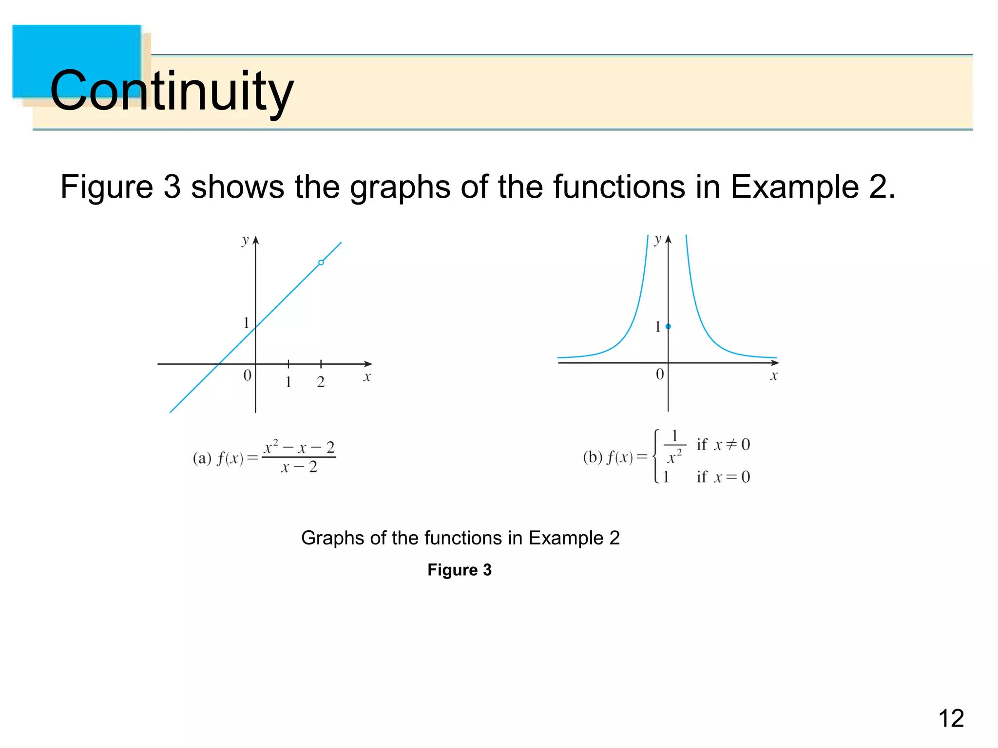
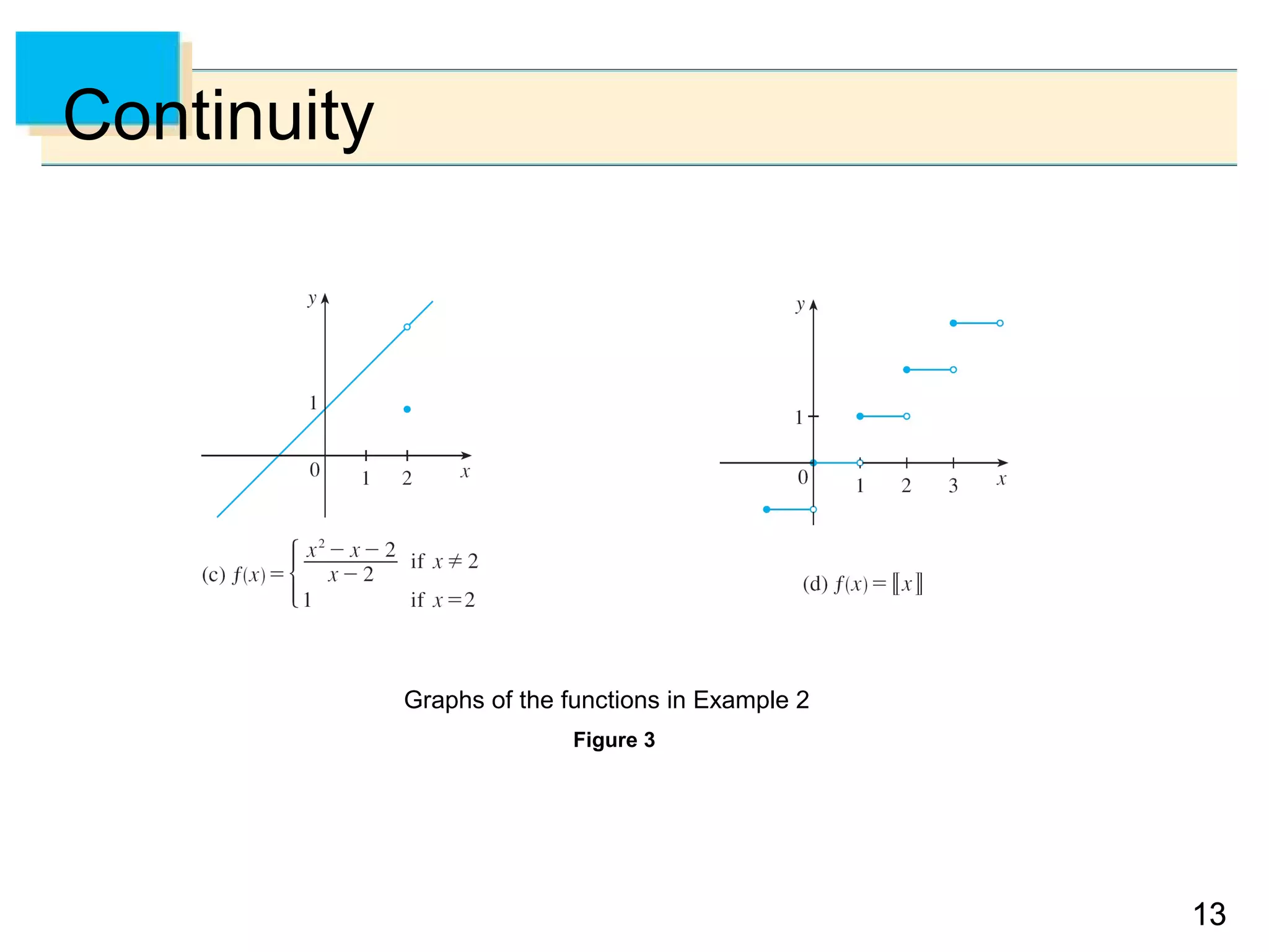
In each case the graph can’t be drawn without lifting the
pen from the paper because a hole or break or jump occurs
in the graph.
The kind of discontinuity illustrated in parts (a) and (c) is
called removable because we could remove the
discontinuity by redefining f at just the single number 2.
[The function g(x) = x + 1 is continuous.]
The discontinuity in part (b) is called an infinite
discontinuity. The discontinuities in part (d) are called
jump discontinuities because the function “jumps” from
one value to another.](https://image.slidesharecdn.com/stewartcalc7e0108-140926231135-phpapp02/75/Stewart-calc7e-01_08-14-2048.jpg)
![2424
Continuity
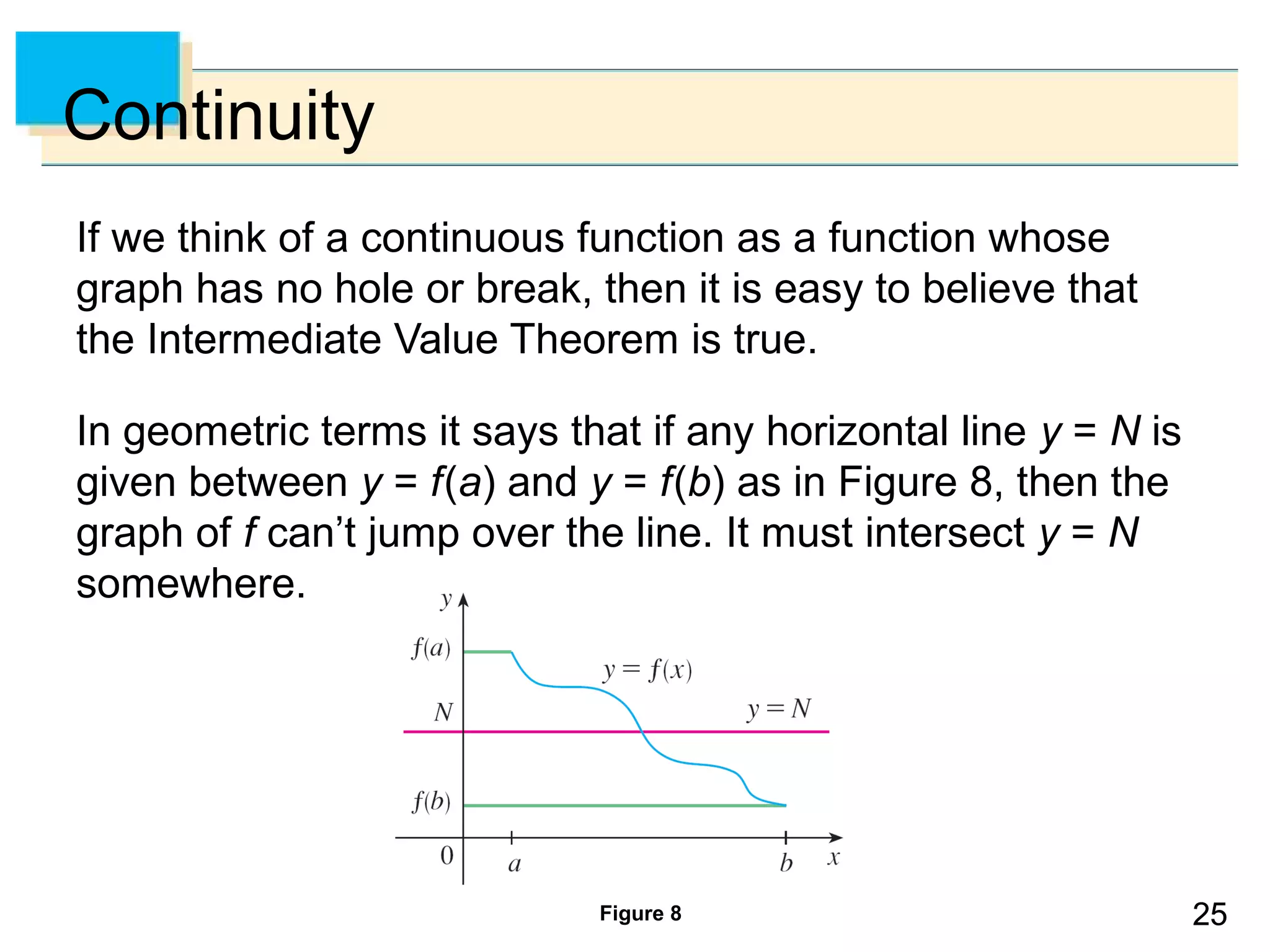
The Intermediate Value Theorem states that a continuous
function takes on every intermediate value between the
function values f(a) and f(b). It is illustrated by Figure 7.
Note that the value N can be taken on once [as in part (a)]
or more than once [as in part (b)].
Figure 7](https://image.slidesharecdn.com/stewartcalc7e0108-140926231135-phpapp02/75/Stewart-calc7e-01_08-24-2048.jpg)
![2626
Continuity
It is important that the function f in Theorem 10 be
continuous. The Intermediate Value Theorem is not true in
general for discontinuous functions.
We can use a graphing calculator or computer to illustrate
the use of the Intermediate Value Theorem.
Figure 9 shows the graph of f in the
viewing rectangle [–1, 3] by [–3, 3] and
you can see that the graph crosses the
x-axis between 1 and 2.
Figure 9](https://image.slidesharecdn.com/stewartcalc7e0108-140926231135-phpapp02/75/Stewart-calc7e-01_08-26-2048.jpg)
![2727
Continuity
Figure 10 shows the result of zooming in to the viewing
rectangle [1.2, 1.3] by [–0.2, 0.2].
In fact, the Intermediate Value Theorem plays a role in the
very way these graphing devices work.
Figure 10](https://image.slidesharecdn.com/stewartcalc7e0108-140926231135-phpapp02/75/Stewart-calc7e-01_08-27-2048.jpg)


![1414
Continuity
In each case the graph can’t be drawn without lifting the
pen from the paper because a hole or break or jump occurs
in the graph.
The kind of discontinuity illustrated in parts (a) and (c) is
called removable because we could remove the
discontinuity by redefining f at just the single number 2.
[The function g(x) = x + 1 is continuous.]
The discontinuity in part (b) is called an infinite
discontinuity. The discontinuities in part (d) are called
jump discontinuities because the function “jumps” from
one value to another.](https://crownmelresort.com/image.slidesharecdn.com/stewartcalc7e0108-140926231135-phpapp02/75/Stewart-calc7e-01_08-14-2048.jpg)


![2424
Continuity
The Intermediate Value Theorem states that a continuous
function takes on every intermediate value between the
function values f(a) and f(b). It is illustrated by Figure 7.
Note that the value N can be taken on once [as in part (a)]
or more than once [as in part (b)].
Figure 7](https://crownmelresort.com/image.slidesharecdn.com/stewartcalc7e0108-140926231135-phpapp02/75/Stewart-calc7e-01_08-24-2048.jpg)

![2626
Continuity
It is important that the function f in Theorem 10 be
continuous. The Intermediate Value Theorem is not true in
general for discontinuous functions.
We can use a graphing calculator or computer to illustrate
the use of the Intermediate Value Theorem.
Figure 9 shows the graph of f in the
viewing rectangle [–1, 3] by [–3, 3] and
you can see that the graph crosses the
x-axis between 1 and 2.
Figure 9](https://crownmelresort.com/image.slidesharecdn.com/stewartcalc7e0108-140926231135-phpapp02/75/Stewart-calc7e-01_08-26-2048.jpg)
![2727
Continuity
Figure 10 shows the result of zooming in to the viewing
rectangle [1.2, 1.3] by [–0.2, 0.2].
In fact, the Intermediate Value Theorem plays a role in the
very way these graphing devices work.
Figure 10](https://crownmelresort.com/image.slidesharecdn.com/stewartcalc7e0108-140926231135-phpapp02/75/Stewart-calc7e-01_08-27-2048.jpg)


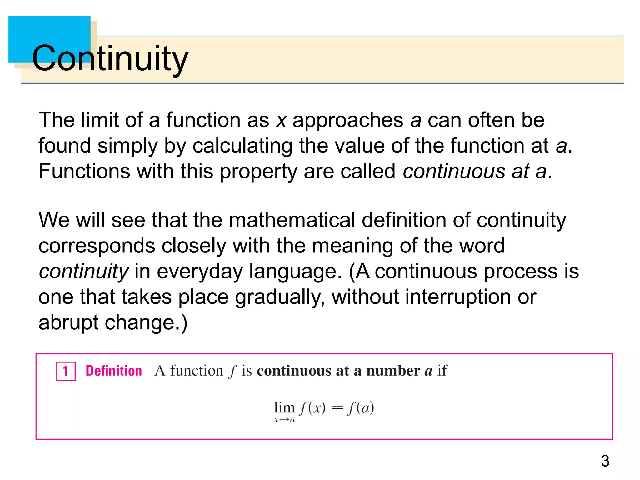
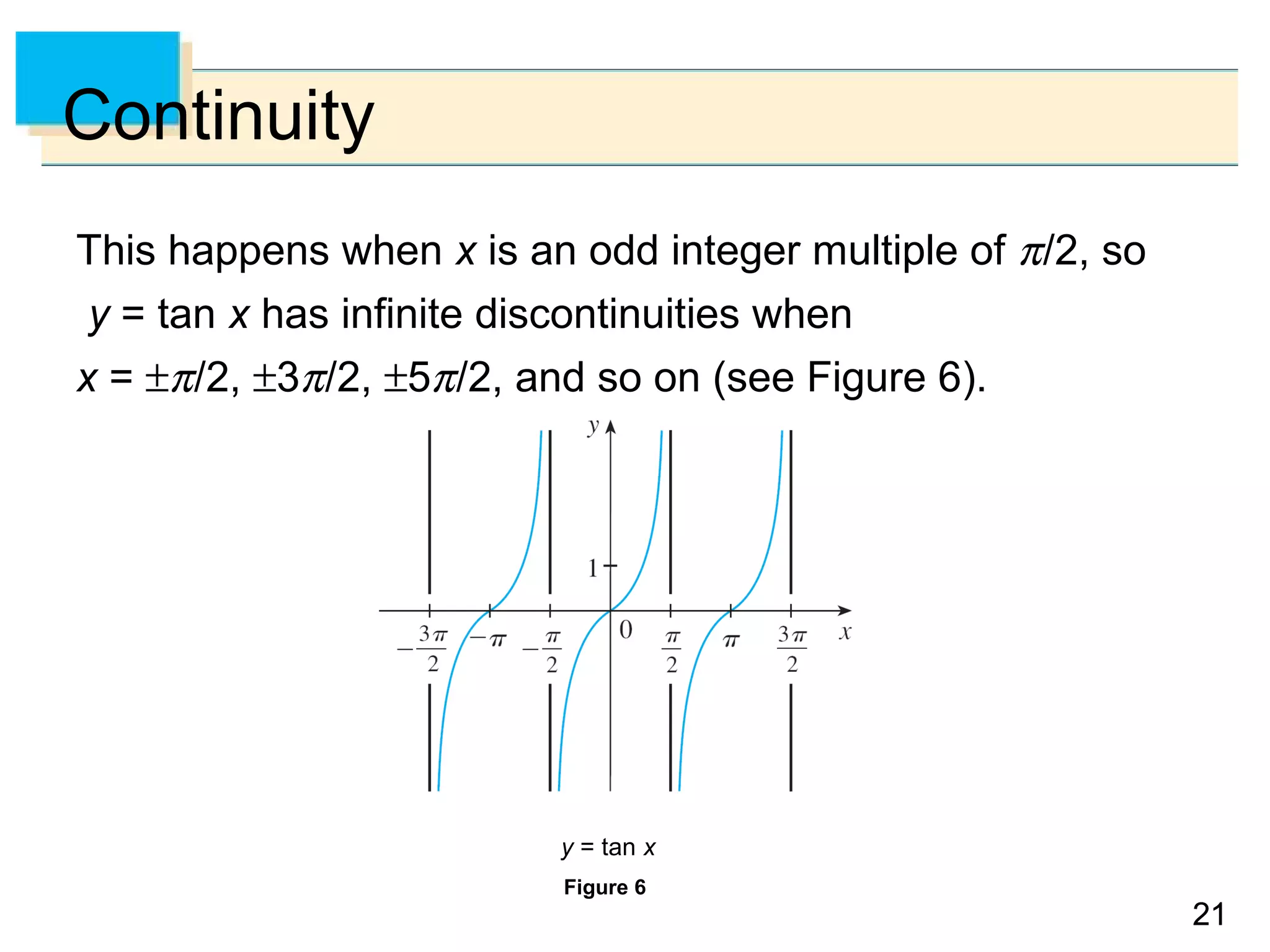
The document discusses continuity of functions. It defines a continuous function as one where the limit of the function as x approaches a number a equals the value of the function at a. A function is discontinuous if this is not true. Continuous functions have graphs that can be drawn without lifting the pen, while discontinuous functions have breaks. The intermediate value theorem states that a continuous function takes on all intermediate values between two function values.


![Limits and continuity[1]](https://cdn.slidesharecdn.com/ss_thumbnails/limitsandcontinuity1-110816105053-phpapp01-thumbnail.jpg?width=640&height=640&fit=bounds)