This document provides an overview of Python for data analysis using the pandas library. It discusses key pandas concepts like Series and DataFrames for working with one-dimensional and multi-dimensional labeled data structures. It also covers common data analysis tasks in pandas such as data loading, aggregation, grouping, pivoting, filtering, handling time series data, and plotting.
• Python forData
Analysis
• Wes McKinney
• Lead developer of
pandas
• Quantitative Financial
Analyst
4.
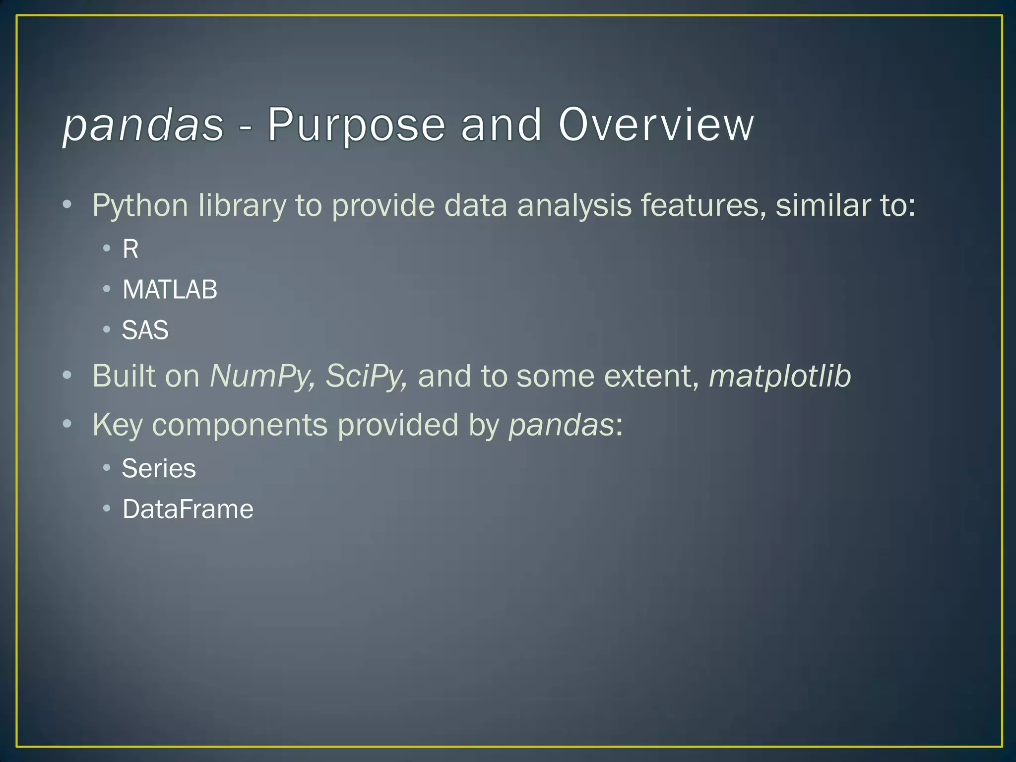
• Python libraryto provide data analysis features, similar to:
• R
• MATLAB
• SAS
• Built on NumPy, SciPy, and to some extent, matplotlib
• Key components provided by pandas:
• Series
• DataFrame
5.
• One-dimensional
array-like object
containingdata
and labels (or
index)
• Lots of ways to
build a Series
>>> import pandas as pd
>>> s = pd.Series(list('abcdef'))
>>> s
0 a
1 b
2 c
3 d
4 e
5 f
>>> s = pd.Series([2, 4, 6, 8])
>>> s
0 2
1 4
2 6
3 8
6.
• A Seriesindex can be
specified
• Single values can be
selected by index
• Multiple values can be
selected with multiple
indexes
>>> s = pd.Series([2, 4, 6, 8],
index = ['f', 'a', 'c', 'e'])
>>>
>>> s
f 2
a 4
c 6
e 8
>>> s['a']
4
>>> s[['a', 'c']]
a 4
c 6
7.
• Think ofa Series as a
fixed-length, ordered
dict
• However, unlike a dict,
index items don't have
to be unique
>>> s2 = pd.Series(range(4),
index = list('abab'))
>>> s2
a 0
b 1
a 2
b 3
>>> s['a]
>>>
>>> s['a']
4
>>> s2['a']
a 0
a 2
>>> s2['a'][0]
0
8.
• Filtering
• NumPy-typeoperations
on data
>>> s
f 2
a 4
c 6
e 8
>>> s[s > 4]
c 6
e 8
>>> s>4
f False
a False
c True
e True
>>> s*2
f 4
a 8
c 12
e 16
9.
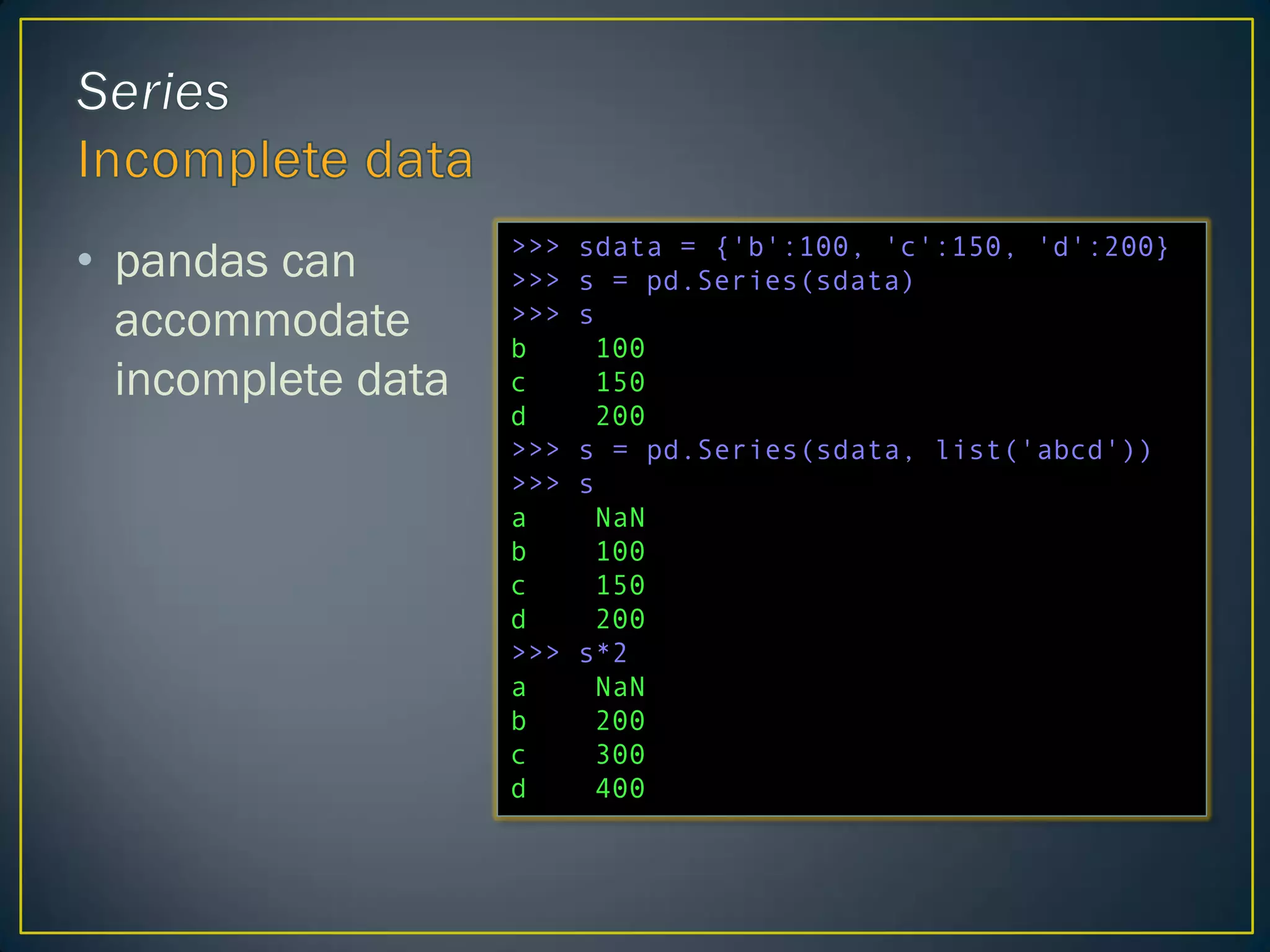
• pandas can
accommodate
incompletedata
>>> sdata = {'b':100, 'c':150, 'd':200}
>>> s = pd.Series(sdata)
>>> s
b 100
c 150
d 200
>>> s = pd.Series(sdata, list('abcd'))
>>> s
a NaN
b 100
c 150
d 200
>>> s*2
a NaN
b 200
c 300
d 400
10.
• Unlike ina NumPy
ndarray, data is
automatically aligned
>>> s2 = pd.Series([1, 2, 3],
index = ['c', 'b', 'a'])
>>> s2
c 1
b 2
a 3
>>> s
a NaN
b 100
c 150
d 200
>>> s*s2
a NaN
b 200
c 150
d NaN
11.
• Spreadsheet-like datastructure containing an
ordered collection of columns
• Has both a row and column index
• Consider as dict of Series (with shared index)
12.
>>> data ={'state': ['FL', 'FL', 'GA', 'GA', 'GA'],
'year': [2010, 2011, 2008, 2010, 2011],
'pop': [18.8, 19.1, 9.7, 9.7, 9.8]}
>>> frame = pd.DataFrame(data)
>>> frame
pop state year
0 18.8 FL 2010
1 19.1 FL 2011
2 9.7 GA 2008
3 9.7 GA 2010
4 9.8 GA 2011
13.
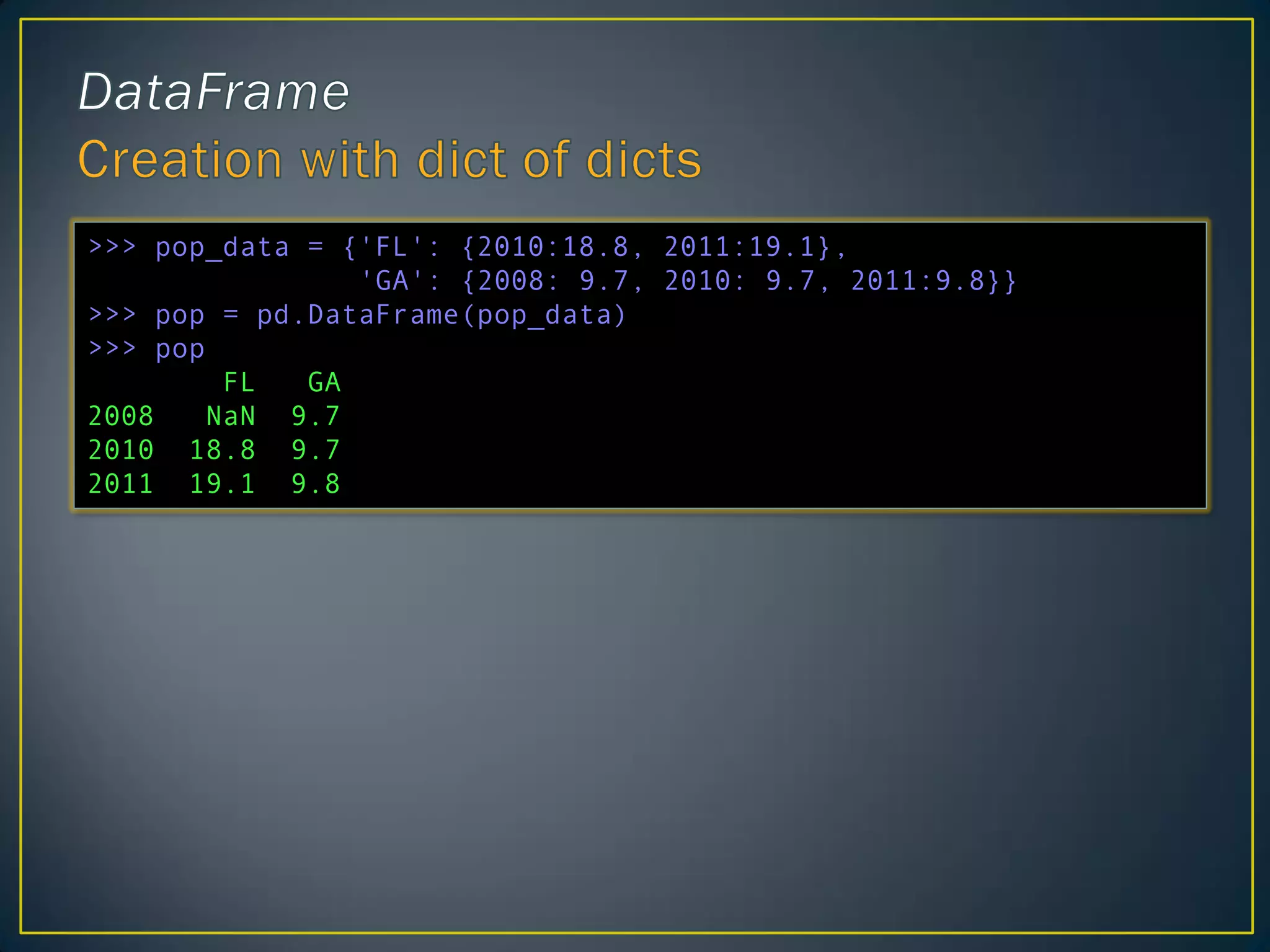
>>> pop_data ={'FL': {2010:18.8, 2011:19.1},
'GA': {2008: 9.7, 2010: 9.7, 2011:9.8}}
>>> pop = pd.DataFrame(pop_data)
>>> pop
FL GA
2008 NaN 9.7
2010 18.8 9.7
2011 19.1 9.8
14.
• Columns canbe retrieved
as a Series
• dict notation
• attribute notation
• Rows can retrieved by
position or by name (using
ix attribute)
>>> frame['state']
0 FL
1 FL
2 GA
3 GA
4 GA
Name: state
>>> frame.describe
<bound method DataFrame.describe
of pop state year
0 18.8 FL 2010
1 19.1 FL 2011
2 9.7 GA 2008
3 9.7 GA 2010
4 9.8 GA 2011>
15.
• New columnscan be
added (by computation
or direct assignment)
>>> frame['other'] = NaN
>>> frame
pop state year other
0 18.8 FL 2010 NaN
1 19.1 FL 2011 NaN
2 9.7 GA 2008 NaN
3 9.7 GA 2010 NaN
4 9.8 GA 2011 NaN
>>> frame['calc'] = frame['pop'] * 2
>>> frame
pop state year other calc
0 18.8 FL 2010 NaN 37.6
1 19.1 FL 2011 NaN 38.2
2 9.7 GA 2008 NaN 19.4
3 9.7 GA 2010 NaN 19.4
4 9.8 GA 2011 NaN 19.6
16.
>>> obj =pd.Series(['blue', 'purple', 'red'],
index=[0,2,4])
>>> obj
0 blue
2 purple
4 red
>>> obj.reindex(range(4))
0 blue
1 NaN
2 purple
3 NaN
>>> obj.reindex(range(5), fill_value='black')
0 blue
1 black
2 purple
3 black
4 red
>>> obj.reindex(range(5), method='ffill')
0 blue
1 blue
2 purple
3 purple
4 red
• Creation of new
object with the
data conformed
to a new index
17.
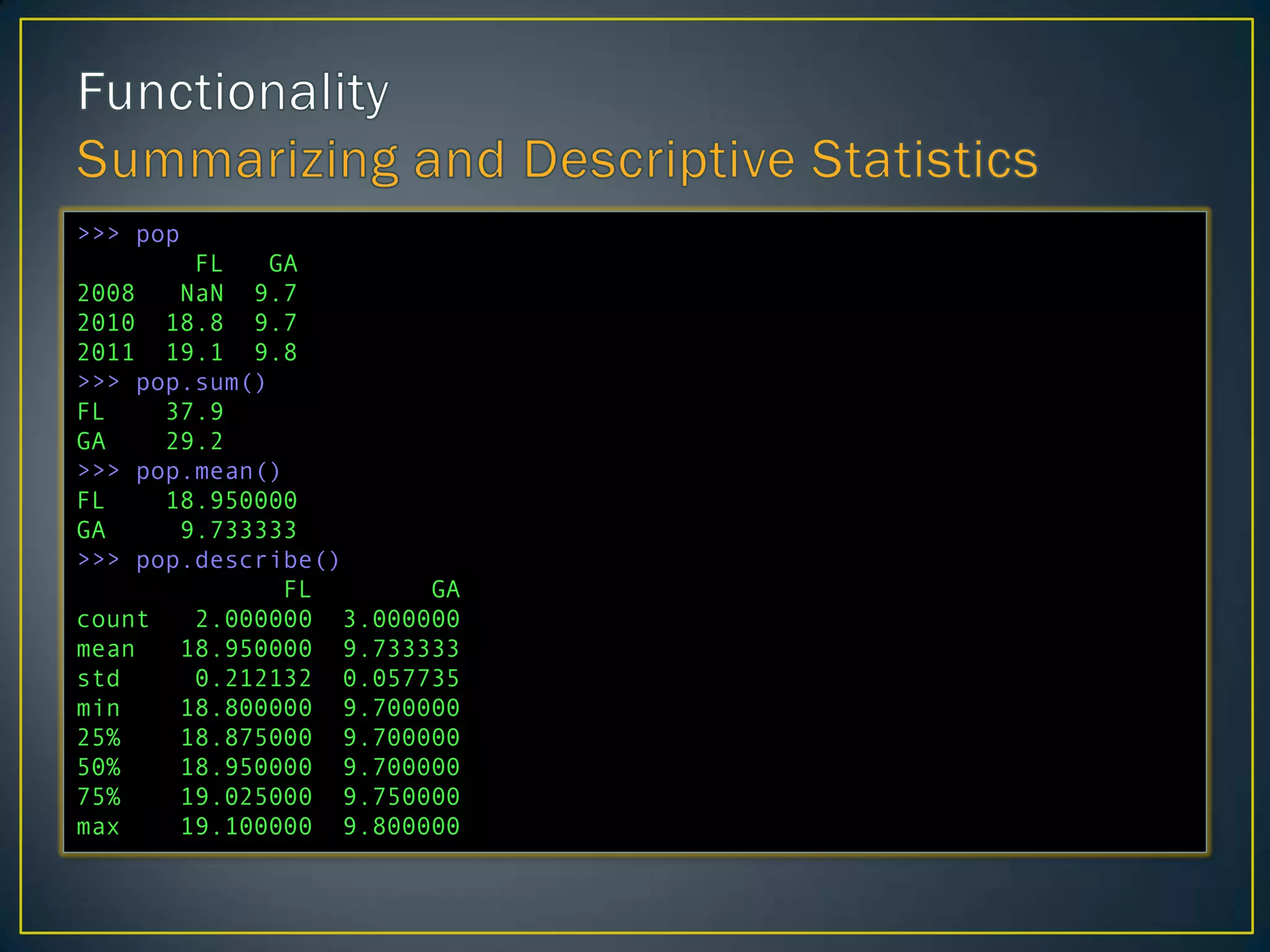
>>> pop
FL GA
2008NaN 9.7
2010 18.8 9.7
2011 19.1 9.8
>>> pop.sum()
FL 37.9
GA 29.2
>>> pop.mean()
FL 18.950000
GA 9.733333
>>> pop.describe()
FL GA
count 2.000000 3.000000
mean 18.950000 9.733333
std 0.212132 0.057735
min 18.800000 9.700000
25% 18.875000 9.700000
50% 18.950000 9.700000
75% 19.025000 9.750000
max 19.100000 9.800000
18.
>>> pop
FL GA
2008NaN 9.7
2010 18.8 9.7
2011 19.1 9.8
>>> pop < 9.8
FL GA
2008 False True
2010 False True
2011 False False
>>> pop[pop < 9.8] = 0
>>> pop
FL GA
2008 NaN 0.0
2010 18.8 0.0
2011 19.1 9.8
19.
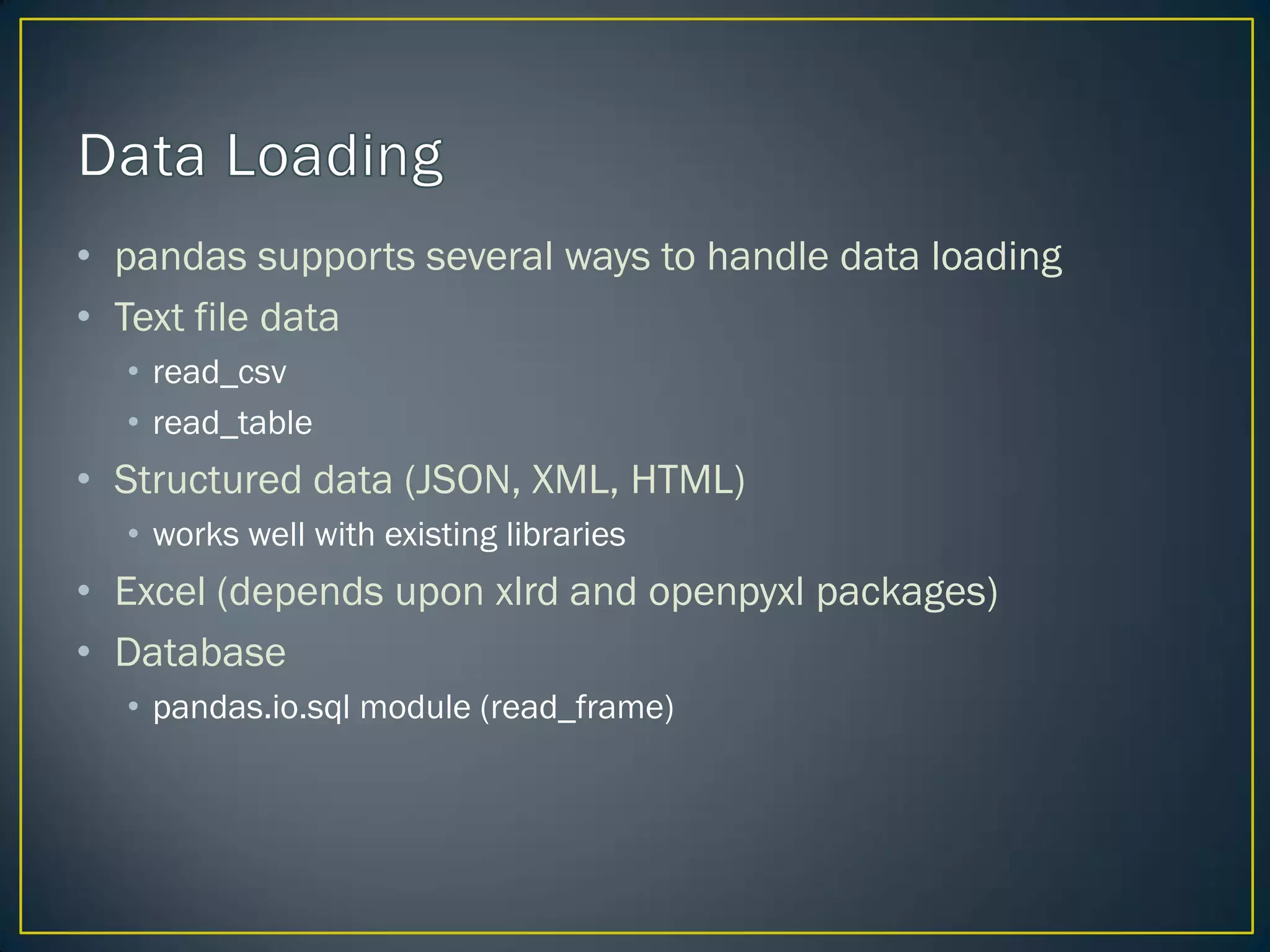
• pandas supportsseveral ways to handle data loading
• Text file data
• read_csv
• read_table
• Structured data (JSON, XML, HTML)
• works well with existing libraries
• Excel (depends upon xlrd and openpyxl packages)
• Database
• pandas.io.sql module (read_frame)
20.
>>> tips =pd.read_csv('/users/ah6/Desktop/pandas
talk/data/tips.csv')
>>> tips.ix[:2]
total_bill tip sex smoker day time size
0 16.99 1.01 Female No Sun Dinner 2
1 10.34 1.66 Male No Sun Dinner 3
2 21.01 3.50 Male No Sun Dinner 3
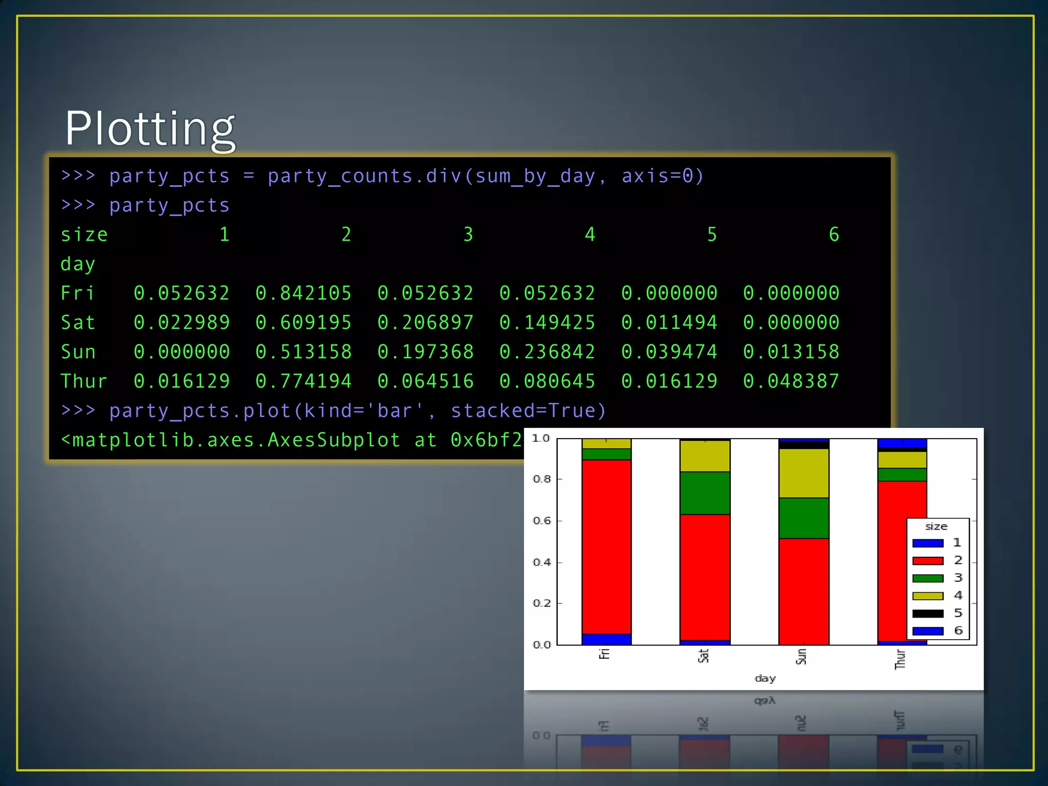
>>> party_counts = pd.crosstab(tips.day, tips.size)
>>> party_counts
size 1 2 3 4 5 6
day
Fri 1 16 1 1 0 0
Sat 2 53 18 13 1 0
Sun 0 39 15 18 3 1
Thur 1 48 4 5 1 3
>>> sum_by_day = party_counts.sum(1).astype(float)
>>> tips['tip_pct'] =tips['tip'] / tips['total_bill']
>>> tips['tip_pct'].hist(bins=50)
<matplotlib.axes.AxesSubplot at 0x6c10d30>
>>> tips['tip_pct'].describe()
count 244.000000
mean 0.160803
std 0.061072
min 0.035638
25% 0.129127
50% 0.154770
75% 0.191475
max 0.710345
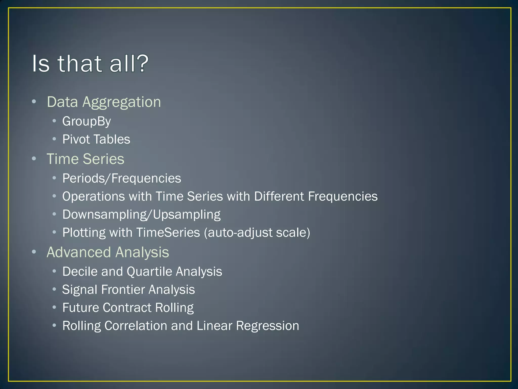
23.
• Data Aggregation
•GroupBy
• Pivot Tables
• Time Series
• Periods/Frequencies
• Operations with Time Series with Different Frequencies
• Downsampling/Upsampling
• Plotting with TimeSeries (auto-adjust scale)
• Advanced Analysis
• Decile and Quartile Analysis
• Signal Frontier Analysis
• Future Contract Rolling
• Rolling Correlation and Linear Regression


![• One-dimensional
array-like object
containing data
and labels (or
index)
• Lots of ways to
build a Series
>>> import pandas as pd
>>> s = pd.Series(list('abcdef'))
>>> s
0 a
1 b
2 c
3 d
4 e
5 f
>>> s = pd.Series([2, 4, 6, 8])
>>> s
0 2
1 4
2 6
3 8](https://image.slidesharecdn.com/pandas-130614111704-phpapp01/75/pandas-Python-Data-Analysis-5-2048.jpg)
![• A Series index can be
specified
• Single values can be
selected by index
• Multiple values can be
selected with multiple
indexes
>>> s = pd.Series([2, 4, 6, 8],
index = ['f', 'a', 'c', 'e'])
>>>
>>> s
f 2
a 4
c 6
e 8
>>> s['a']
4
>>> s[['a', 'c']]
a 4
c 6](https://image.slidesharecdn.com/pandas-130614111704-phpapp01/75/pandas-Python-Data-Analysis-6-2048.jpg)
![• Think of a Series as a
fixed-length, ordered
dict
• However, unlike a dict,
index items don't have
to be unique
>>> s2 = pd.Series(range(4),
index = list('abab'))
>>> s2
a 0
b 1
a 2
b 3
>>> s['a]
>>>
>>> s['a']
4
>>> s2['a']
a 0
a 2
>>> s2['a'][0]
0](https://image.slidesharecdn.com/pandas-130614111704-phpapp01/75/pandas-Python-Data-Analysis-7-2048.jpg)
![• Filtering
• NumPy-type operations
on data
>>> s
f 2
a 4
c 6
e 8
>>> s[s > 4]
c 6
e 8
>>> s>4
f False
a False
c True
e True
>>> s*2
f 4
a 8
c 12
e 16](https://image.slidesharecdn.com/pandas-130614111704-phpapp01/75/pandas-Python-Data-Analysis-8-2048.jpg)
![• Unlike in a NumPy
ndarray, data is
automatically aligned
>>> s2 = pd.Series([1, 2, 3],
index = ['c', 'b', 'a'])
>>> s2
c 1
b 2
a 3
>>> s
a NaN
b 100
c 150
d 200
>>> s*s2
a NaN
b 200
c 150
d NaN](https://image.slidesharecdn.com/pandas-130614111704-phpapp01/75/pandas-Python-Data-Analysis-10-2048.jpg)
![>>> data = {'state': ['FL', 'FL', 'GA', 'GA', 'GA'],
'year': [2010, 2011, 2008, 2010, 2011],
'pop': [18.8, 19.1, 9.7, 9.7, 9.8]}
>>> frame = pd.DataFrame(data)
>>> frame
pop state year
0 18.8 FL 2010
1 19.1 FL 2011
2 9.7 GA 2008
3 9.7 GA 2010
4 9.8 GA 2011](https://image.slidesharecdn.com/pandas-130614111704-phpapp01/75/pandas-Python-Data-Analysis-12-2048.jpg)
![• Columns can be retrieved
as a Series
• dict notation
• attribute notation
• Rows can retrieved by
position or by name (using
ix attribute)
>>> frame['state']
0 FL
1 FL
2 GA
3 GA
4 GA
Name: state
>>> frame.describe
<bound method DataFrame.describe
of pop state year
0 18.8 FL 2010
1 19.1 FL 2011
2 9.7 GA 2008
3 9.7 GA 2010
4 9.8 GA 2011>](https://image.slidesharecdn.com/pandas-130614111704-phpapp01/75/pandas-Python-Data-Analysis-14-2048.jpg)
![• New columns can be
added (by computation
or direct assignment)
>>> frame['other'] = NaN
>>> frame
pop state year other
0 18.8 FL 2010 NaN
1 19.1 FL 2011 NaN
2 9.7 GA 2008 NaN
3 9.7 GA 2010 NaN
4 9.8 GA 2011 NaN
>>> frame['calc'] = frame['pop'] * 2
>>> frame
pop state year other calc
0 18.8 FL 2010 NaN 37.6
1 19.1 FL 2011 NaN 38.2
2 9.7 GA 2008 NaN 19.4
3 9.7 GA 2010 NaN 19.4
4 9.8 GA 2011 NaN 19.6](https://image.slidesharecdn.com/pandas-130614111704-phpapp01/75/pandas-Python-Data-Analysis-15-2048.jpg)
![>>> obj = pd.Series(['blue', 'purple', 'red'],
index=[0,2,4])
>>> obj
0 blue
2 purple
4 red
>>> obj.reindex(range(4))
0 blue
1 NaN
2 purple
3 NaN
>>> obj.reindex(range(5), fill_value='black')
0 blue
1 black
2 purple
3 black
4 red
>>> obj.reindex(range(5), method='ffill')
0 blue
1 blue
2 purple
3 purple
4 red
• Creation of new
object with the
data conformed
to a new index](https://image.slidesharecdn.com/pandas-130614111704-phpapp01/75/pandas-Python-Data-Analysis-16-2048.jpg)
![>>> pop
FL GA
2008 NaN 9.7
2010 18.8 9.7
2011 19.1 9.8
>>> pop < 9.8
FL GA
2008 False True
2010 False True
2011 False False
>>> pop[pop < 9.8] = 0
>>> pop
FL GA
2008 NaN 0.0
2010 18.8 0.0
2011 19.1 9.8](https://image.slidesharecdn.com/pandas-130614111704-phpapp01/75/pandas-Python-Data-Analysis-18-2048.jpg)
![>>> tips = pd.read_csv('/users/ah6/Desktop/pandas
talk/data/tips.csv')
>>> tips.ix[:2]
total_bill tip sex smoker day time size
0 16.99 1.01 Female No Sun Dinner 2
1 10.34 1.66 Male No Sun Dinner 3
2 21.01 3.50 Male No Sun Dinner 3
>>> party_counts = pd.crosstab(tips.day, tips.size)
>>> party_counts
size 1 2 3 4 5 6
day
Fri 1 16 1 1 0 0
Sat 2 53 18 13 1 0
Sun 0 39 15 18 3 1
Thur 1 48 4 5 1 3
>>> sum_by_day = party_counts.sum(1).astype(float)](https://image.slidesharecdn.com/pandas-130614111704-phpapp01/75/pandas-Python-Data-Analysis-20-2048.jpg)
![>>> tips['tip_pct'] = tips['tip'] / tips['total_bill']
>>> tips['tip_pct'].hist(bins=50)
<matplotlib.axes.AxesSubplot at 0x6c10d30>
>>> tips['tip_pct'].describe()
count 244.000000
mean 0.160803
std 0.061072
min 0.035638
25% 0.129127
50% 0.154770
75% 0.191475
max 0.710345](https://image.slidesharecdn.com/pandas-130614111704-phpapp01/75/pandas-Python-Data-Analysis-22-2048.jpg)


![• One-dimensional
array-like object
containing data
and labels (or
index)
• Lots of ways to
build a Series
>>> import pandas as pd
>>> s = pd.Series(list('abcdef'))
>>> s
0 a
1 b
2 c
3 d
4 e
5 f
>>> s = pd.Series([2, 4, 6, 8])
>>> s
0 2
1 4
2 6
3 8](https://crownmelresort.com/image.slidesharecdn.com/pandas-130614111704-phpapp01/75/pandas-Python-Data-Analysis-5-2048.jpg)
![• A Series index can be
specified
• Single values can be
selected by index
• Multiple values can be
selected with multiple
indexes
>>> s = pd.Series([2, 4, 6, 8],
index = ['f', 'a', 'c', 'e'])
>>>
>>> s
f 2
a 4
c 6
e 8
>>> s['a']
4
>>> s[['a', 'c']]
a 4
c 6](https://crownmelresort.com/image.slidesharecdn.com/pandas-130614111704-phpapp01/75/pandas-Python-Data-Analysis-6-2048.jpg)
![• Think of a Series as a
fixed-length, ordered
dict
• However, unlike a dict,
index items don't have
to be unique
>>> s2 = pd.Series(range(4),
index = list('abab'))
>>> s2
a 0
b 1
a 2
b 3
>>> s['a]
>>>
>>> s['a']
4
>>> s2['a']
a 0
a 2
>>> s2['a'][0]
0](https://crownmelresort.com/image.slidesharecdn.com/pandas-130614111704-phpapp01/75/pandas-Python-Data-Analysis-7-2048.jpg)
![• Filtering
• NumPy-type operations
on data
>>> s
f 2
a 4
c 6
e 8
>>> s[s > 4]
c 6
e 8
>>> s>4
f False
a False
c True
e True
>>> s*2
f 4
a 8
c 12
e 16](https://crownmelresort.com/image.slidesharecdn.com/pandas-130614111704-phpapp01/75/pandas-Python-Data-Analysis-8-2048.jpg)

![• Unlike in a NumPy
ndarray, data is
automatically aligned
>>> s2 = pd.Series([1, 2, 3],
index = ['c', 'b', 'a'])
>>> s2
c 1
b 2
a 3
>>> s
a NaN
b 100
c 150
d 200
>>> s*s2
a NaN
b 200
c 150
d NaN](https://crownmelresort.com/image.slidesharecdn.com/pandas-130614111704-phpapp01/75/pandas-Python-Data-Analysis-10-2048.jpg)

![>>> data = {'state': ['FL', 'FL', 'GA', 'GA', 'GA'],
'year': [2010, 2011, 2008, 2010, 2011],
'pop': [18.8, 19.1, 9.7, 9.7, 9.8]}
>>> frame = pd.DataFrame(data)
>>> frame
pop state year
0 18.8 FL 2010
1 19.1 FL 2011
2 9.7 GA 2008
3 9.7 GA 2010
4 9.8 GA 2011](https://crownmelresort.com/image.slidesharecdn.com/pandas-130614111704-phpapp01/75/pandas-Python-Data-Analysis-12-2048.jpg)

![• Columns can be retrieved
as a Series
• dict notation
• attribute notation
• Rows can retrieved by
position or by name (using
ix attribute)
>>> frame['state']
0 FL
1 FL
2 GA
3 GA
4 GA
Name: state
>>> frame.describe
<bound method DataFrame.describe
of pop state year
0 18.8 FL 2010
1 19.1 FL 2011
2 9.7 GA 2008
3 9.7 GA 2010
4 9.8 GA 2011>](https://crownmelresort.com/image.slidesharecdn.com/pandas-130614111704-phpapp01/75/pandas-Python-Data-Analysis-14-2048.jpg)
![• New columns can be
added (by computation
or direct assignment)
>>> frame['other'] = NaN
>>> frame
pop state year other
0 18.8 FL 2010 NaN
1 19.1 FL 2011 NaN
2 9.7 GA 2008 NaN
3 9.7 GA 2010 NaN
4 9.8 GA 2011 NaN
>>> frame['calc'] = frame['pop'] * 2
>>> frame
pop state year other calc
0 18.8 FL 2010 NaN 37.6
1 19.1 FL 2011 NaN 38.2
2 9.7 GA 2008 NaN 19.4
3 9.7 GA 2010 NaN 19.4
4 9.8 GA 2011 NaN 19.6](https://crownmelresort.com/image.slidesharecdn.com/pandas-130614111704-phpapp01/75/pandas-Python-Data-Analysis-15-2048.jpg)
![>>> obj = pd.Series(['blue', 'purple', 'red'],
index=[0,2,4])
>>> obj
0 blue
2 purple
4 red
>>> obj.reindex(range(4))
0 blue
1 NaN
2 purple
3 NaN
>>> obj.reindex(range(5), fill_value='black')
0 blue
1 black
2 purple
3 black
4 red
>>> obj.reindex(range(5), method='ffill')
0 blue
1 blue
2 purple
3 purple
4 red
• Creation of new
object with the
data conformed
to a new index](https://crownmelresort.com/image.slidesharecdn.com/pandas-130614111704-phpapp01/75/pandas-Python-Data-Analysis-16-2048.jpg)

![>>> pop
FL GA
2008 NaN 9.7
2010 18.8 9.7
2011 19.1 9.8
>>> pop < 9.8
FL GA
2008 False True
2010 False True
2011 False False
>>> pop[pop < 9.8] = 0
>>> pop
FL GA
2008 NaN 0.0
2010 18.8 0.0
2011 19.1 9.8](https://crownmelresort.com/image.slidesharecdn.com/pandas-130614111704-phpapp01/75/pandas-Python-Data-Analysis-18-2048.jpg)

![>>> tips = pd.read_csv('/users/ah6/Desktop/pandas
talk/data/tips.csv')
>>> tips.ix[:2]
total_bill tip sex smoker day time size
0 16.99 1.01 Female No Sun Dinner 2
1 10.34 1.66 Male No Sun Dinner 3
2 21.01 3.50 Male No Sun Dinner 3
>>> party_counts = pd.crosstab(tips.day, tips.size)
>>> party_counts
size 1 2 3 4 5 6
day
Fri 1 16 1 1 0 0
Sat 2 53 18 13 1 0
Sun 0 39 15 18 3 1
Thur 1 48 4 5 1 3
>>> sum_by_day = party_counts.sum(1).astype(float)](https://crownmelresort.com/image.slidesharecdn.com/pandas-130614111704-phpapp01/75/pandas-Python-Data-Analysis-20-2048.jpg)

![>>> tips['tip_pct'] = tips['tip'] / tips['total_bill']
>>> tips['tip_pct'].hist(bins=50)
<matplotlib.axes.AxesSubplot at 0x6c10d30>
>>> tips['tip_pct'].describe()
count 244.000000
mean 0.160803
std 0.061072
min 0.035638
25% 0.129127
50% 0.154770
75% 0.191475
max 0.710345](https://crownmelresort.com/image.slidesharecdn.com/pandas-130614111704-phpapp01/75/pandas-Python-Data-Analysis-22-2048.jpg)


![Introduction to Pandas and Time Series Analysis [PyCon DE]](https://cdn.slidesharecdn.com/ss_thumbnails/introductiontopandasandtimeseriesanalysispyconde-170617163724-thumbnail.jpg?width=640&height=640&fit=bounds)