Download to read offline


![Vectors
[2,3] = + 3 x [0,1]
2 x [1,0]
2 x + 3 x
e1 e2
2 x + 3 x
x = [2,3] Can be arbitrary # of
dimensions
(typically denoted Rn
)](https://image.slidesharecdn.com/04math-241123011744-b40b74c3/75/Numerical-Linear-Algebra-in-digital-image-processing-26-2048.jpg)
![Vectors
x = [2,3]
𝒙 =
[2
3]
𝒙1=2
𝒙2=3
Just an array!
Get in the habit of thinking of
them as columns.](https://image.slidesharecdn.com/04math-241123011744-b40b74c3/75/Numerical-Linear-Algebra-in-digital-image-processing-27-2048.jpg)
![Scaling Vectors
x = [2,3]
2x = [4,6] • Can scale vector by a scalar
• Scalar = single number
• Dimensions changed
independently
• Changes magnitude / length,
does not change direction.](https://image.slidesharecdn.com/04math-241123011744-b40b74c3/75/Numerical-Linear-Algebra-in-digital-image-processing-28-2048.jpg)
![Adding Vectors
y = [3,1]
x+y = [5,4]
x = [2,3]
• Can add vectors
• Dimensions changed independently
• Order irrelevant
• Can change direction and magnitude](https://image.slidesharecdn.com/04math-241123011744-b40b74c3/75/Numerical-Linear-Algebra-in-digital-image-processing-29-2048.jpg)
![Scaling and Adding
y = [3,1]
2x+y = [7,7]
Can do both at the same
time
x = [2,3]](https://image.slidesharecdn.com/04math-241123011744-b40b74c3/75/Numerical-Linear-Algebra-in-digital-image-processing-30-2048.jpg)
![Measuring Length
y = [3,1]
x = [2,3]
Magnitude / length / (L2) norm of vector
‖𝒙‖=‖𝒙‖2=
(∑
𝑖
𝑛
𝑥𝑖
2
)
1/2
There are other norms; assume L2
unless told otherwise
‖𝒙‖2=√13
‖𝒚‖2 =√10
Why?](https://image.slidesharecdn.com/04math-241123011744-b40b74c3/75/Numerical-Linear-Algebra-in-digital-image-processing-31-2048.jpg)
![Normalizing a Vector
x = [2,3]
y = [3,1]
𝒙′
=𝒙 /‖𝒙‖𝟐
𝒚′
= 𝒚 /‖𝒚‖𝟐
Diving by norm gives
something on the unit
sphere (all vectors with
length 1)](https://image.slidesharecdn.com/04math-241123011744-b40b74c3/75/Numerical-Linear-Algebra-in-digital-image-processing-32-2048.jpg)
![Dot Products
𝒆𝟏
𝒆𝟐
𝒙⋅𝒚 =∑
𝑖
𝑛
𝑥𝑖 𝑦𝑖
𝒙=[2,3]
What’s , ?
Ans: ;
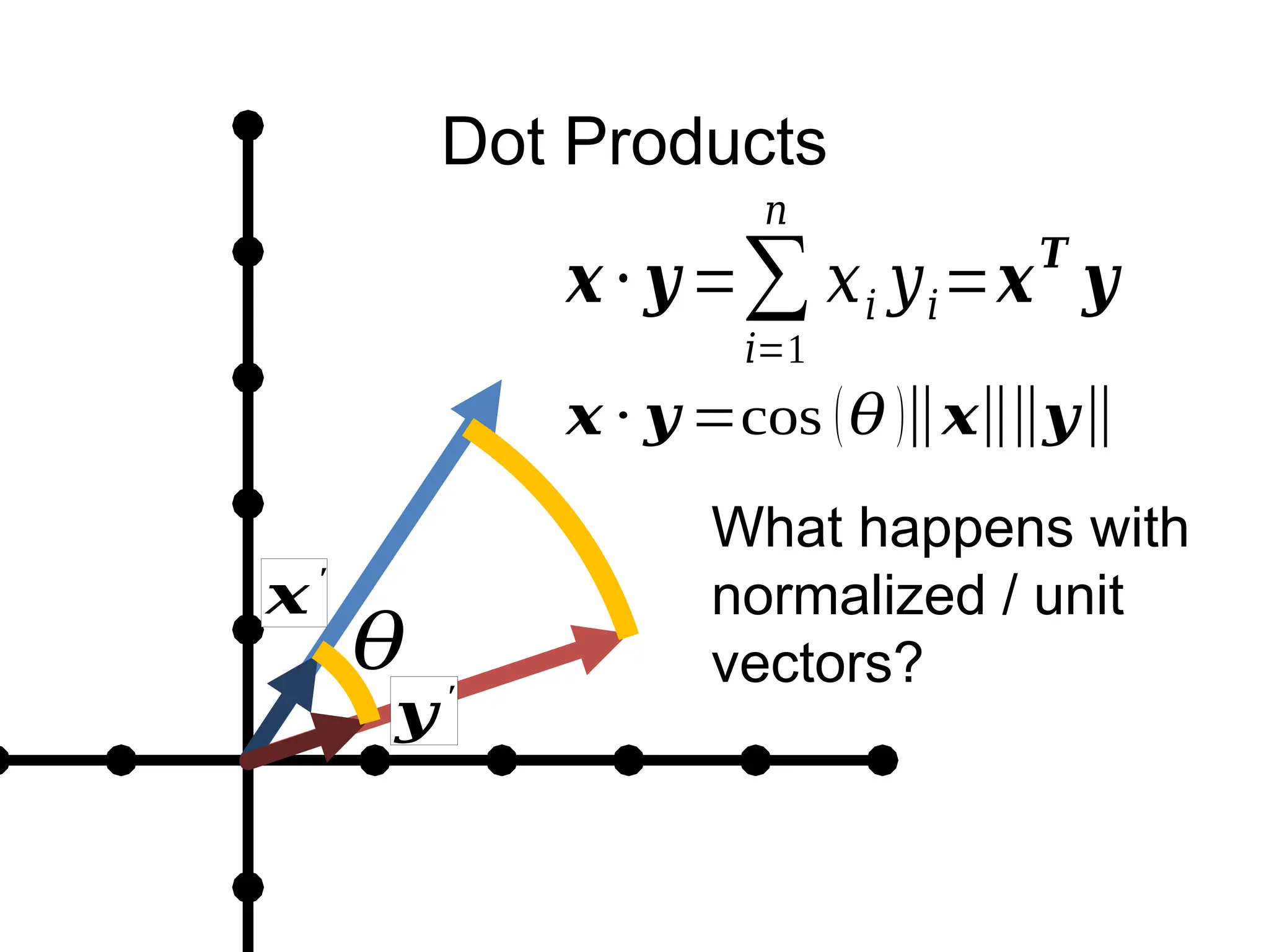
• Dot product is projection
• Amount of x that’s also
pointing in direction of y](https://image.slidesharecdn.com/04math-241123011744-b40b74c3/75/Numerical-Linear-Algebra-in-digital-image-processing-34-2048.jpg)
![Dot Products
What’s ?
Ans:
𝒙⋅𝒚 =∑
𝑖
𝑛
𝑥𝑖 𝑦𝑖
𝒙=[2,3]](https://image.slidesharecdn.com/04math-241123011744-b40b74c3/75/Numerical-Linear-Algebra-in-digital-image-processing-35-2048.jpg)
![Special Angles
𝒙′
𝒚′
𝜃
[1
0 ]⋅[0
1 ]=0 ∗1+ 1∗ 0=0
Perpendicular /
orthogonal vectors
have dot product 0
irrespective of their
magnitude
𝒙
𝒚](https://image.slidesharecdn.com/04math-241123011744-b40b74c3/75/Numerical-Linear-Algebra-in-digital-image-processing-36-2048.jpg)
![Special Angles
[𝑥1
𝑥2
]⋅
[𝑦1
𝑦2
]=𝑥1 𝑦 1+ 𝑥2 𝑦2=0
Perpendicular /
orthogonal vectors
have dot product 0
irrespective of their
magnitude
𝒙′
𝒚′
𝜃
𝒙
𝒚](https://image.slidesharecdn.com/04math-241123011744-b40b74c3/75/Numerical-Linear-Algebra-in-digital-image-processing-37-2048.jpg)
![Orthogonal Vectors
𝒙=[2,3]
• Geometrically,
what’s the set of
vectors that are
orthogonal to x?
• A line [3,-2]](https://image.slidesharecdn.com/04math-241123011744-b40b74c3/75/Numerical-Linear-Algebra-in-digital-image-processing-38-2048.jpg)
![Orthogonal Vectors
• What’s the set of vectors that are
orthogonal to x = [5,0,0]?
• A plane/2D space of vectors/any
vector
• What’s the set of vectors that are
orthogonal to x and y = [0,5,0]?
• A line/1D space of vectors/any
vector
• Ambiguity in sign and magnitude
𝒙
𝒙
𝒚](https://image.slidesharecdn.com/04math-241123011744-b40b74c3/75/Numerical-Linear-Algebra-in-digital-image-processing-39-2048.jpg)
![Matrices
Horizontally concatenate n, m-dim column vectors
and you get a mxn matrix A (here 2x3)
𝑨=[ 𝒗1 ,⋯ , 𝒗 𝑛]=
[𝑣11
𝑣21
𝑣31
𝑣12
𝑣22
𝑣32
]
a
(scalar)
lowercase
undecorated
a
(vector)
lowercase
bold or arrow
A
(matrix)
uppercase
bold](https://image.slidesharecdn.com/04math-241123011744-b40b74c3/75/Numerical-Linear-Algebra-in-digital-image-processing-42-2048.jpg)
![Matrices
Vertically concatenate m, n-dim row vectors
and you get a mxn matrix A (here 2x3)
𝐴=
[
𝒖1
𝑇
⋮
𝒖𝑛
𝑇 ]=
[𝑢11
𝑢12
𝑢13
𝑢21
𝑢22
𝑢23
]
Transpose: flip
rows / columns [
𝑎
𝑏
𝑐 ]
𝑇
=[𝑎 𝑏 𝑐 ] (3x1)T
= 1x3](https://image.slidesharecdn.com/04math-241123011744-b40b74c3/75/Numerical-Linear-Algebra-in-digital-image-processing-43-2048.jpg)
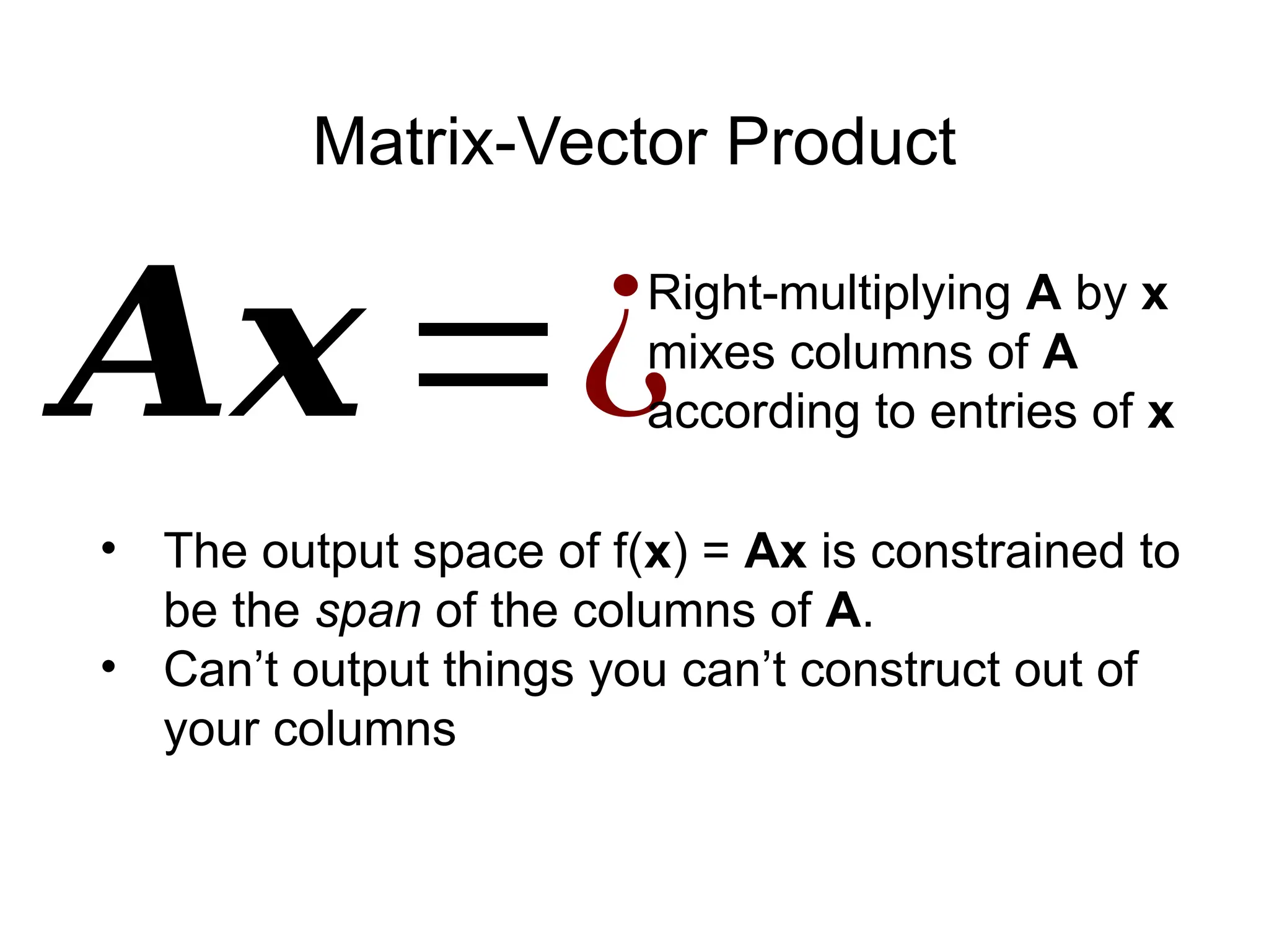
![Matrix-Vector Product
𝒚2 𝑥1= 𝑨2 𝑥3 𝒙3 𝑥 1
𝒚 =𝑥1 𝒗𝟏 +𝑥2 𝒗𝟐 +𝑥3 𝒗𝟑
Linear combination of columns of A
[𝑦1
𝑦2
]=¿[𝒗𝟏 𝒗𝟐 𝒗𝟑 ][
𝑥1
𝑥2
𝑥3
]](https://image.slidesharecdn.com/04math-241123011744-b40b74c3/75/Numerical-Linear-Algebra-in-digital-image-processing-44-2048.jpg)
![Matrix-Vector Product
𝒚2 𝑥1= 𝑨2 𝑥3 𝒙3 𝑥 1
𝑦 1=𝒖𝟏
𝑻
𝒙
Dot product between rows of A and x
𝑦 2=𝒖𝟐
𝑻
𝒙
[𝒖𝟏
𝑻
𝒖𝟐
𝑻
]
[𝑦1
𝑦2
]=¿ 𝒙
3
3](https://image.slidesharecdn.com/04math-241123011744-b40b74c3/75/Numerical-Linear-Algebra-in-digital-image-processing-45-2048.jpg)
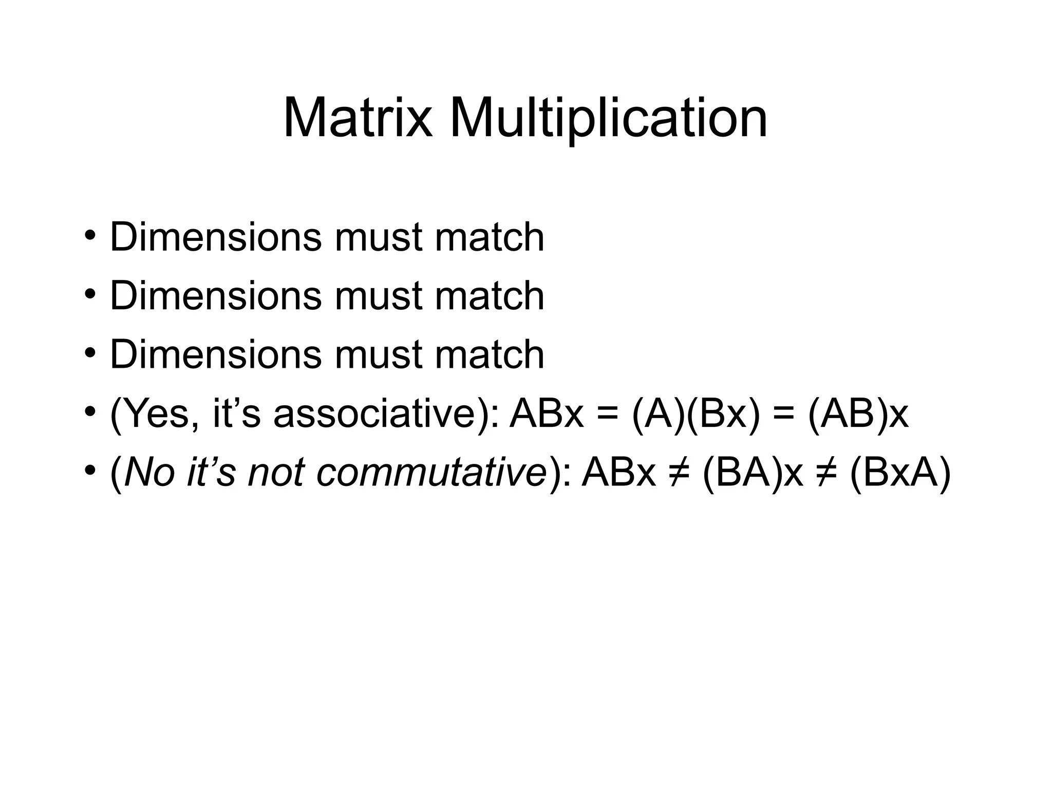
![Matrix Multiplication
[− 𝒂𝟏
𝑻
−
¿⋮ ¿− ¿
−¿
]¿
𝑨𝑩=¿
Generally: Amn and Bnp yield product (AB)mp
Yes – in A, I’m referring to the rows, and in B,
I’m referring to the columns](https://image.slidesharecdn.com/04math-241123011744-b40b74c3/75/Numerical-Linear-Algebra-in-digital-image-processing-46-2048.jpg)
![Matrix Multiplication
[− 𝒂𝟏
𝑻
−
¿⋮ ¿− ¿
−¿
]
¿
𝑨𝑩=¿
[
𝒂𝟏
𝑻
𝒃𝟏 ⋯ 𝒂𝟏
𝑻
𝒃𝒑
⋮ ⋱ ⋮
𝒂𝒎
𝑻
𝒃𝟏 ⋯ 𝒂𝒎
𝑻
𝒃𝒑
]
𝑨 𝑩𝑖𝑗=𝒂𝒊
𝑻
𝒃𝒋
Generally: Amn and Bnp yield product (AB)mp](https://image.slidesharecdn.com/04math-241123011744-b40b74c3/75/Numerical-Linear-Algebra-in-digital-image-processing-47-2048.jpg)
![Operations They Don’t Teach
[𝑎+𝑒 𝑏+𝑒
𝑐 +𝑒 𝑑+𝑒]
[𝑎 𝑏
𝑐 𝑑]+
[𝑒 𝑓
𝑔 h]=¿
[𝑎+𝑒 𝑏+ 𝑓
𝑐+𝑔 𝑑+h ]
You Probably Saw Matrix Addition
[𝑎 𝑏
𝑐 𝑑]+𝑒=¿
What is this? FYI: e is a scalar](https://image.slidesharecdn.com/04math-241123011744-b40b74c3/75/Numerical-Linear-Algebra-in-digital-image-processing-49-2048.jpg)
![Broadcasting
[𝑎 𝑏
𝑐 𝑑]+𝑒
¿
[𝑎 𝑏
𝑐 𝑑 ]+
[𝑒 𝑒
𝑒 𝑒]
¿
[𝑎 𝑏
𝑐 𝑑 ]+𝟏2 𝑥 2 𝑒
If you want to be pedantic and proper, you expand
e by multiplying a matrix of 1s (denoted 1)
Many smart matrix libraries do this automatically.
This is the source of many bugs.](https://image.slidesharecdn.com/04math-241123011744-b40b74c3/75/Numerical-Linear-Algebra-in-digital-image-processing-50-2048.jpg)
![Broadcasting Example
𝑷 =
[
𝑥1 𝑦1
⋮ ⋮
𝑥𝑛 𝑦𝑛
] 𝒗 =
[𝑎
𝑏]
Given: a nx2 matrix P and a 2D column vector v,
Want: nx2 difference matrix D
𝑫=
[
𝑥1 − 𝑎 𝑦1 − 𝑏
⋮ ⋮
𝑥𝑛 − 𝑎 𝑦𝑛 − 𝑏]
𝑷 −𝒗𝑇
=¿
[
𝑥1 𝑦1
⋮ ⋮
𝑥𝑛 𝑦𝑛
]−
[𝑎 𝑏]
[𝑎 𝑏]
⋮
Blue stuff is
assumed /
broadcast](https://image.slidesharecdn.com/04math-241123011744-b40b74c3/75/Numerical-Linear-Algebra-in-digital-image-processing-51-2048.jpg)
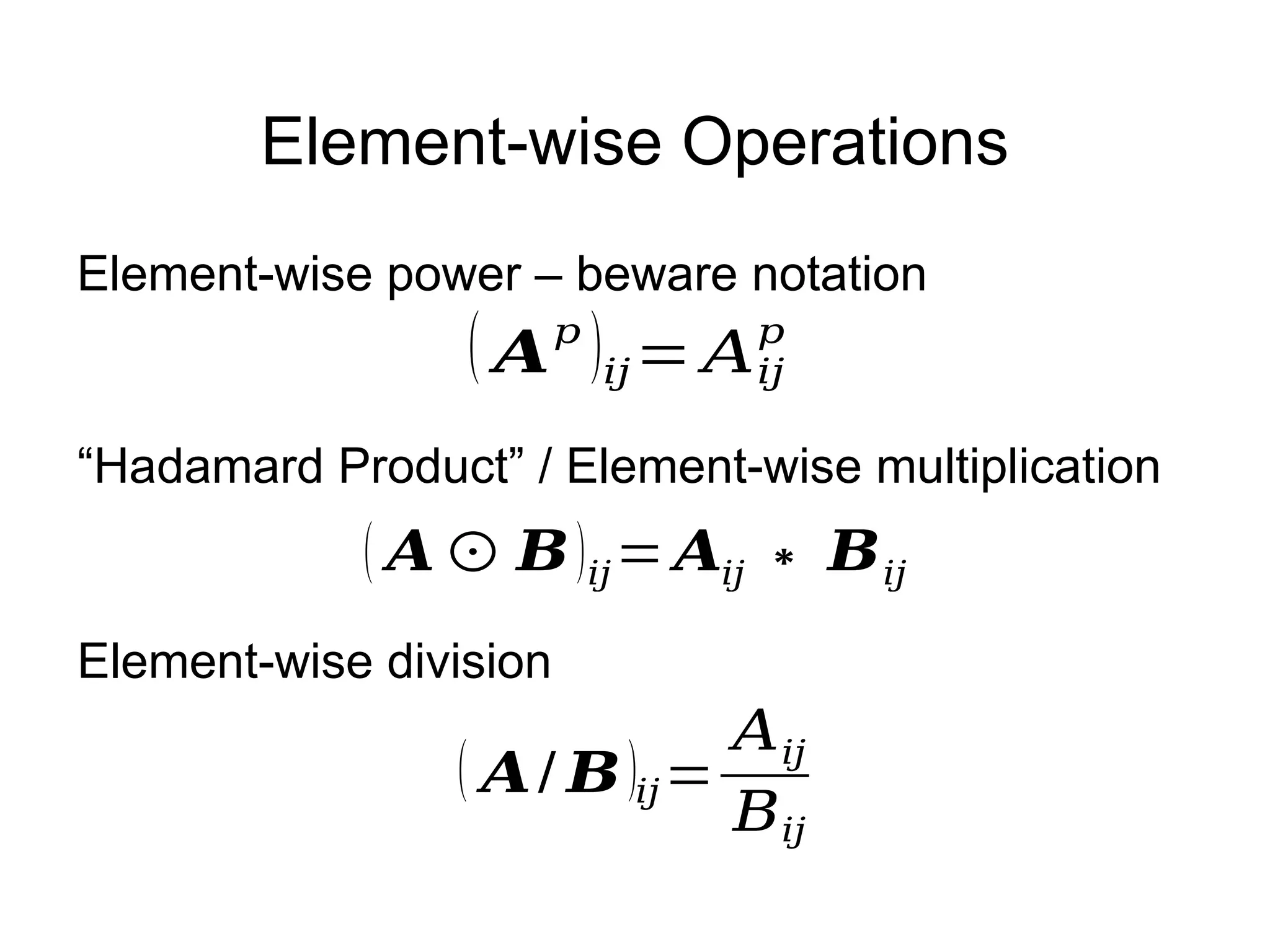
![Implementation
imNew = im**4
Python+Numpy (right way):
Python+Numpy (slow way – why? ):
imNew = np.zeros(im.shape)
for y in range(im.shape[0]):
for x in range(im.shape[1]):
imNew[y,x] = im[y,x]**expFactor](https://image.slidesharecdn.com/04math-241123011744-b40b74c3/75/Numerical-Linear-Algebra-in-digital-image-processing-56-2048.jpg)
![Implementation
imNew = im**4
Python+Numpy (right way):
Python+Numpy (slow way – why? ):
imNew = np.zeros(im.shape)
for y in range(im.shape[0]):
for x in range(im.shape[1]):
imNew[y,x] = im[y,x]**expFactor](https://image.slidesharecdn.com/04math-241123011744-b40b74c3/75/Numerical-Linear-Algebra-in-digital-image-processing-60-2048.jpg)
![Sums Across Axes
𝑨=
[
𝑥1 𝑦1
⋮ ⋮
𝑥𝑛 𝑦𝑛
]
Suppose have
Nx2 matrix A
Σ( 𝑨 ,1)=
[
𝑥1 +𝑦1
⋮
𝑥𝑛 +𝑦𝑛
]
ND col. vec.
Σ( 𝑨 ,0)=
[∑
𝑖=1
𝑛
𝑥𝑖 ,∑
𝑖=1
𝑛
𝑦𝑖
]
2D row vec
Note – libraries distinguish between N-D column vector and Nx1 matrix.](https://image.slidesharecdn.com/04math-241123011744-b40b74c3/75/Numerical-Linear-Algebra-in-digital-image-processing-62-2048.jpg)
![Vectorizing Example
𝑿=
[− 𝒙1 −
¿⋮ ¿− ¿
−¿]𝒀=
[− 𝒚1 −
¿⋮ ¿− ¿
−¿]
(𝑿 𝒀𝑻
)𝑖𝑗=𝒙𝒊
𝑻
𝒚 𝒋
𝒀 𝑻
=¿
𝚺( 𝑿
𝟐
,𝟏)=
[
‖𝒙𝟏‖
𝟐
⋮
‖𝒙𝑵‖
𝟐 ]
Compute a Nx1
vector of norms
(can also do Mx1)
Compute a NxM
matrix of dot products](https://image.slidesharecdn.com/04math-241123011744-b40b74c3/75/Numerical-Linear-Algebra-in-digital-image-processing-64-2048.jpg)
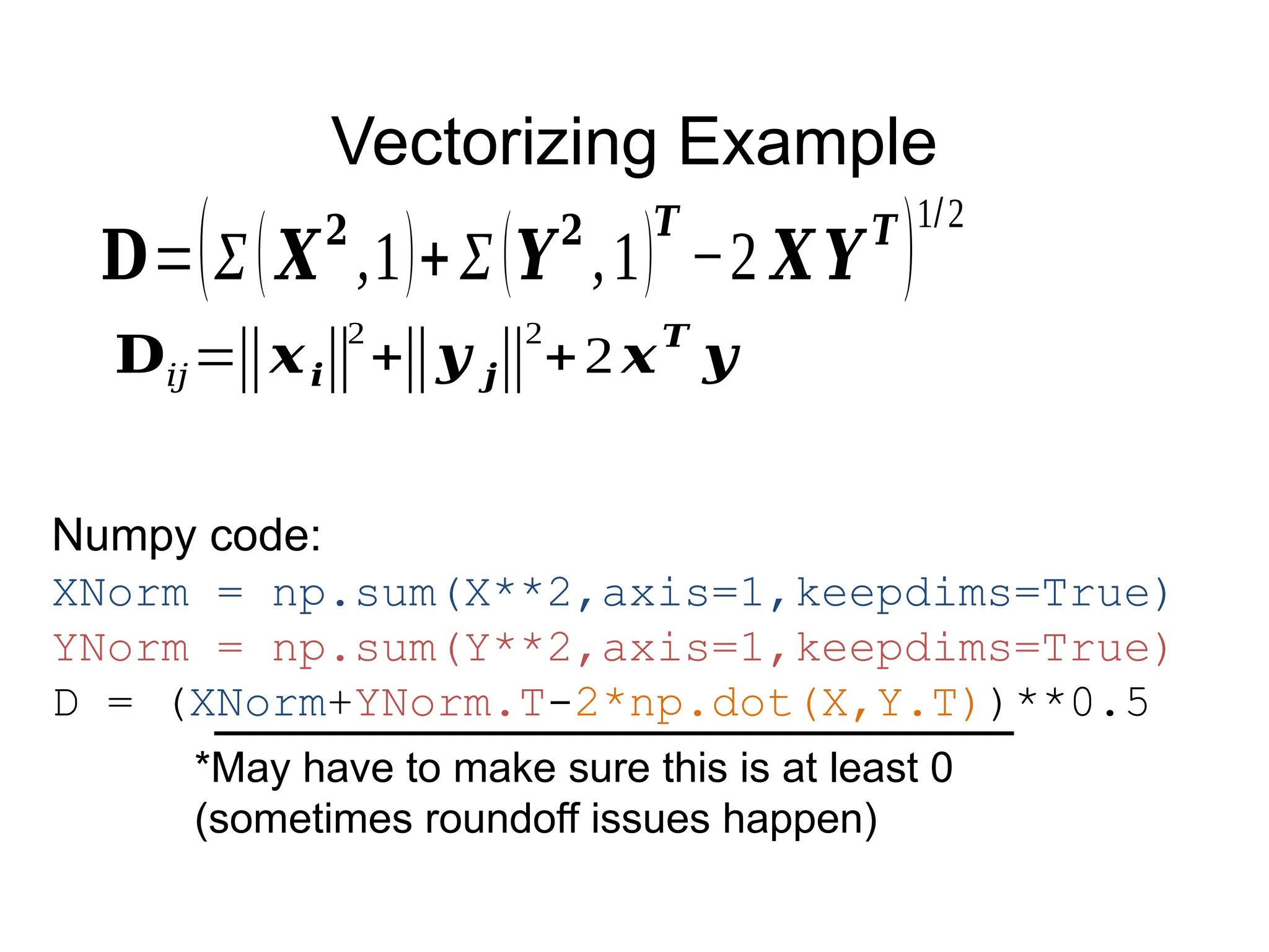
![Vectorizing Example
𝐃=(Σ(𝑿
𝟐
,1)+Σ(𝒀
𝟐
,1)
𝑻
−2 𝑿𝒀
𝑻
)
1/2
[
‖𝒙𝟏‖
𝟐
⋮
‖𝒙 𝑵‖
𝟐 ]+[‖𝒚 1‖
𝟐
⋯ ‖𝒚 𝑀‖
𝟐
]
(Σ( 𝑿
2
, 1)+Σ (𝒀
2
,1)
𝑇
)𝑖𝑗=‖𝒙𝑖‖
2
+‖𝒚 𝑗‖
2
[
‖𝒙𝟏‖
2
+‖𝒚 𝟏‖
2
⋯ ‖𝒙𝟏‖
2
+‖𝒚 𝑴‖
2
⋮ ⋱ ⋮
‖𝒙 𝑵‖
2
+‖𝒚 𝟏‖
2
⋯ ‖𝒙 𝑵‖
2
+‖𝒚 𝑴‖
2 ] Why?](https://image.slidesharecdn.com/04math-241123011744-b40b74c3/75/Numerical-Linear-Algebra-in-digital-image-processing-65-2048.jpg)
![Linear Independence
𝒚 =
[
0
− 2
1 ]=¿
1
2
𝒂−
1
3
𝒃
𝒙 =
[
0
0
4 ]=¿
2𝒂
• Is the set {a,b,c} linearly independent?
• Is the set {a,b,x} linearly independent?
• Max # of independent 3D vectors?
𝒂=
[
0
0
2 ]𝒃=
[
0
6
0]𝒄=
[
5
0
0]
Suppose:
A set of vectors is linearly independent if you can’t
write one as a linear combination of the others.](https://image.slidesharecdn.com/04math-241123011744-b40b74c3/75/Numerical-Linear-Algebra-in-digital-image-processing-68-2048.jpg)
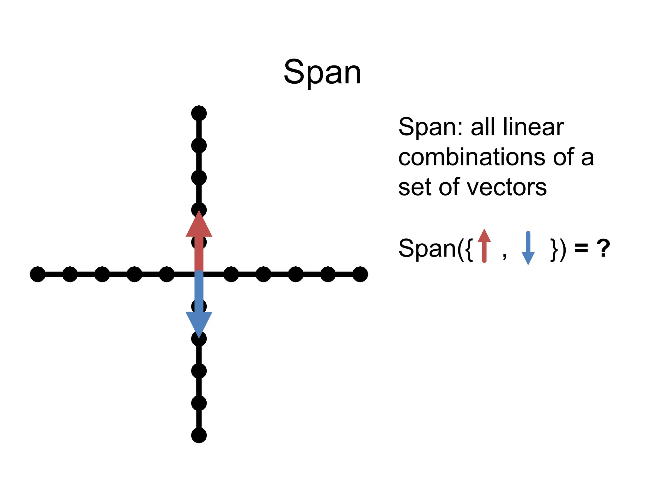
![Span
Span: all linear
combinations of a
set of vectors
Span({ }) =
Span({[0,2]}) = ?
All vertical lines
through origin =
Is blue in {red}’s
span?](https://image.slidesharecdn.com/04math-241123011744-b40b74c3/75/Numerical-Linear-Algebra-in-digital-image-processing-69-2048.jpg)

![An Intuition
x
Ax
y1
y2
y3
x1 x2 x3
y
𝒚 = 𝑨𝒙=
[
¿ ¿ ¿
𝒄𝟏 𝒄𝟐 𝒄𝒏
¿ ¿ ¿
][
𝑥1
𝑥2
𝑥3
]
x – knobs on machine (e.g., fuel, brakes)
y – state of the world (e.g., where you are)
A – machine (e.g., your car)](https://image.slidesharecdn.com/04math-241123011744-b40b74c3/75/Numerical-Linear-Algebra-in-digital-image-processing-73-2048.jpg)
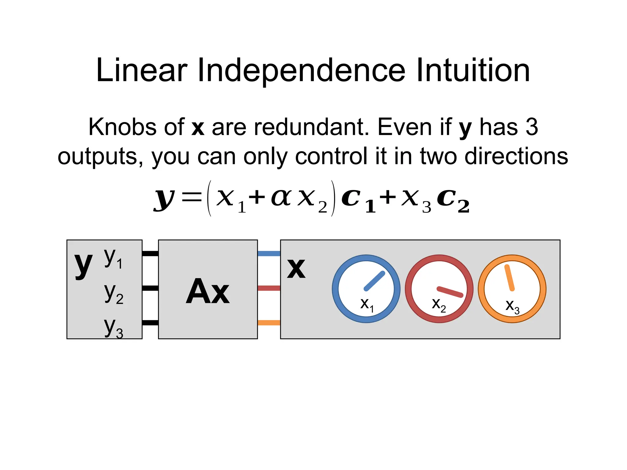
![Linear Independence
𝒚 = 𝑨𝒙=
[
¿ ¿ ¿
𝒄𝟏 𝛼 𝒄𝟏 𝒄𝟐
¿ ¿ ¿
][
𝑥1
𝑥2
𝑥3
]
Suppose the columns of 3x3 matrix A are not
linearly independent (c1, αc1, c2 for instance)
𝒚 =𝑥1 𝒄𝟏+𝛼 𝑥2 𝒄𝟏+𝑥3 𝒄𝟐
𝒚 =(𝑥1+𝛼 𝑥2)𝒄𝟏+𝑥3 𝒄𝟐](https://image.slidesharecdn.com/04math-241123011744-b40b74c3/75/Numerical-Linear-Algebra-in-digital-image-processing-74-2048.jpg)
![Linear Independence
𝑨𝒙 =( 𝑥1 + 𝛼 𝑥 2 ) 𝒄 𝟏+ 𝑥 3 𝒄𝟐
• Or, given a vector y there’s not a unique
vector x s.t. y =Ax
• Not all y have a corresponding x s.t. y=Ax
𝒚 = 𝑨
[
𝑥1+ 𝛽
𝑥2 − 𝛽 /𝛼
𝑥3
]
• Can write y an infinite number of ways by
adding to x1 and subtracting from x2
Recall:
¿(𝑥1+ 𝛽+𝛼 𝑥2− 𝛼
𝛽
𝛼 )𝑐1+𝑥3 𝑐2](https://image.slidesharecdn.com/04math-241123011744-b40b74c3/75/Numerical-Linear-Algebra-in-digital-image-processing-76-2048.jpg)
![Linear Independence
𝑨𝒙 =( 𝑥1 + 𝛼 𝑥 2 ) 𝒄 𝟏+ 𝑥 3 𝒄𝟐
• An infinite number of non-zero vectors x can
map to a zero-vector y
• Called the right null-space of A.
𝒚 = 𝑨
[
𝛽
− 𝛽 / 𝛼
0 ]
¿(𝛽− 𝛼
𝛽
𝛼)𝒄𝟏+0𝒄𝟐
• What else can we cancel out?](https://image.slidesharecdn.com/04math-241123011744-b40b74c3/75/Numerical-Linear-Algebra-in-digital-image-processing-77-2048.jpg)
![Symmetric Matrices
• Symmetric: or
• Have lots of special
properties [
𝑎11 𝑎12 𝑎13
𝑎21 𝑎22 𝑎23
𝑎31 𝑎32 𝑎33
]
Any matrix of the form is symmetric.
Quick check: 𝑨
𝑻
=(𝑿
𝑻
𝑿)𝑻
𝑨
𝑻
=𝑿
𝑻
(𝑿
𝑻
)𝑻
𝑨𝑻
=𝑿𝑻
𝑿](https://image.slidesharecdn.com/04math-241123011744-b40b74c3/75/Numerical-Linear-Algebra-in-digital-image-processing-80-2048.jpg)
![Special Matrices – Rotations
[
𝑟1 1 𝑟12 𝑟 13
𝑟 21 𝑟22 𝑟 23
𝑟 31 𝑟32 𝑟 33
]
• Rotation matrices rotate vectors and do not
change vector L2 norms ()
• Every row/column is unit norm
• Every row is linearly independent
• Transpose is inverse
• Determinant is 1 (otherwise it’s also a coordinate
flip/reflection), eigenvalues are 1](https://image.slidesharecdn.com/04math-241123011744-b40b74c3/75/Numerical-Linear-Algebra-in-digital-image-processing-81-2048.jpg)
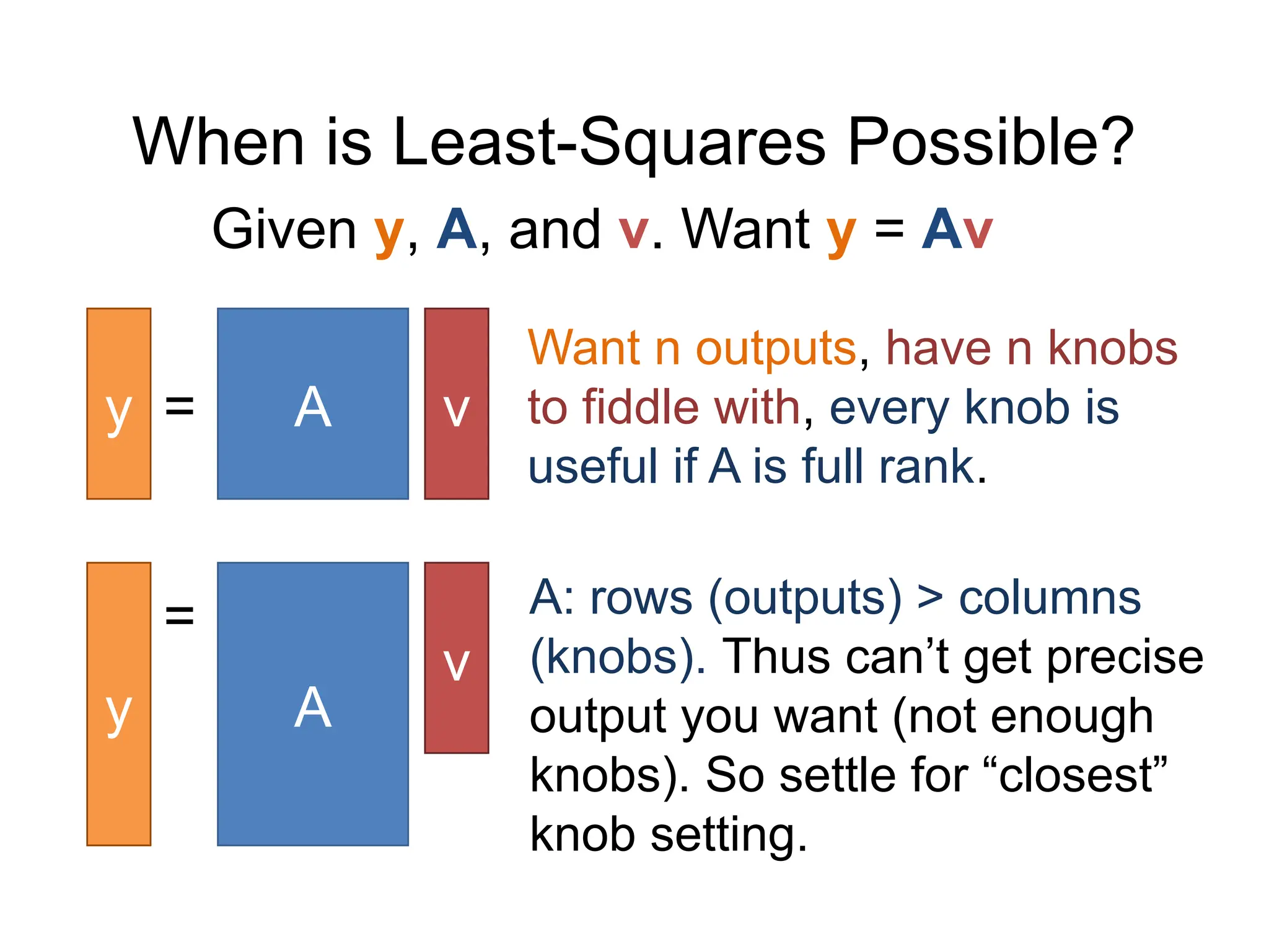
![Red box – unit square, Blue box – after f(x) = Ax.
What are the yellow lines and why?
𝑨=¿
[1.1 0
0 1.1]](https://image.slidesharecdn.com/04math-241123011744-b40b74c3/75/Numerical-Linear-Algebra-in-digital-image-processing-85-2048.jpg)
![𝑨=¿
[0 .8 0
0 1.25]
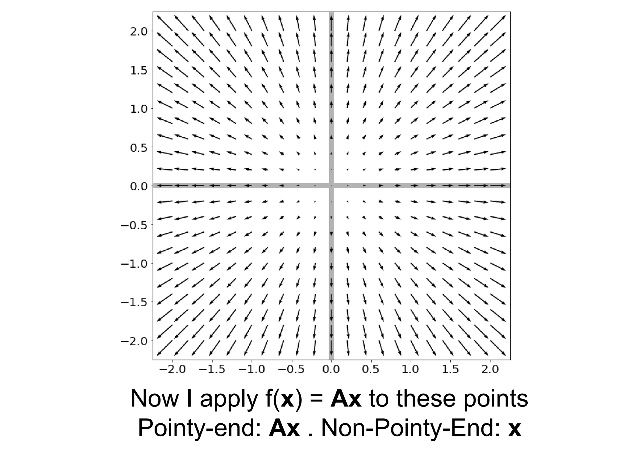
Now I apply f(x) = Ax to these points
Pointy-end: Ax . Non-Pointy-End: x](https://image.slidesharecdn.com/04math-241123011744-b40b74c3/75/Numerical-Linear-Algebra-in-digital-image-processing-86-2048.jpg)
![Red box – unit square, Blue box – after f(x) = Ax.
What are the yellow lines and why?
𝑨=¿
[0 .8 0
0 1.25]](https://image.slidesharecdn.com/04math-241123011744-b40b74c3/75/Numerical-Linear-Algebra-in-digital-image-processing-87-2048.jpg)
![Red box – unit square, Blue box – after f(x) = Ax.
Can we draw any yellow lines?
𝑨=¿
[c os (𝑡) − sin (𝑡)
sin (𝑡) cos (𝑡) ]](https://image.slidesharecdn.com/04math-241123011744-b40b74c3/75/Numerical-Linear-Algebra-in-digital-image-processing-88-2048.jpg)

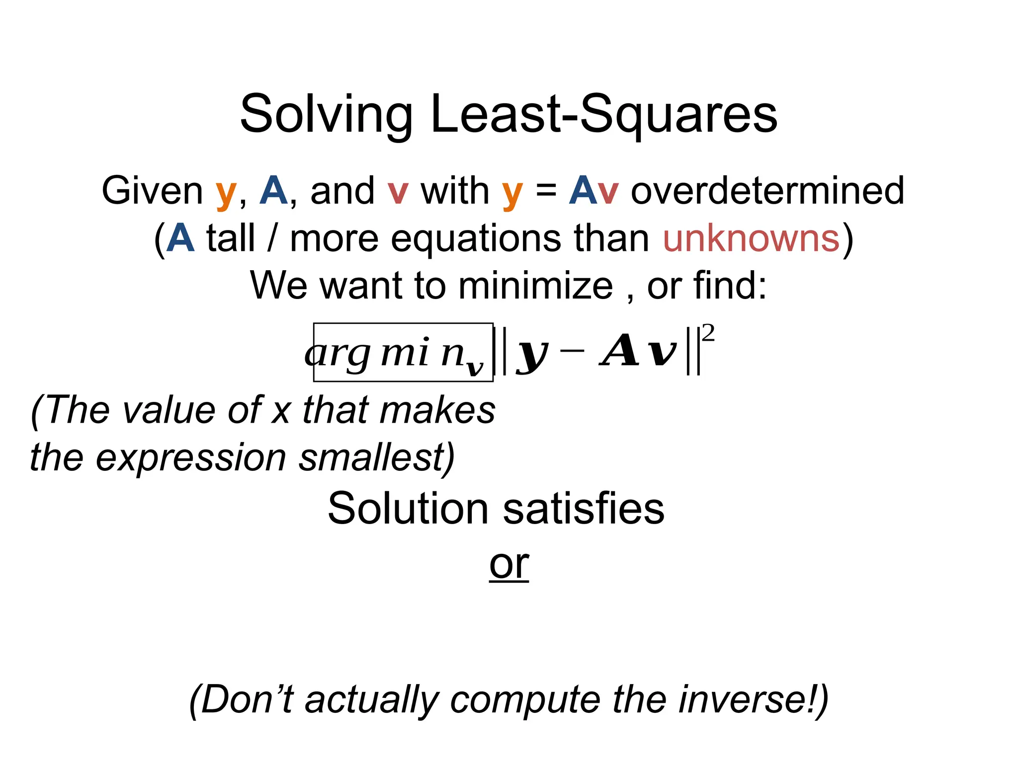
![Solving Least-Squares
Start with two points (xi,yi)
[𝑦1
𝑦2
]=
[𝑥1 1
𝑥2 1 ][𝑚
𝑏 ]
𝒚 =𝑨𝒗
[𝑦1
𝑦2
]=
[𝑚 𝑥1 +𝑏
𝑚 𝑥2 +𝑏 ]
We know how to solve this –
invert A and find v (i.e., (m,b)
that fits points)
(x1,y1)
(x2,y2)](https://image.slidesharecdn.com/04math-241123011744-b40b74c3/75/Numerical-Linear-Algebra-in-digital-image-processing-95-2048.jpg)
![Solving Least-Squares
Start with two points (xi,yi)
[𝑦1
𝑦2
]=
[𝑥1 1
𝑥2 1 ][𝑚
𝑏 ]
𝒚 =𝑨𝒗
‖[𝑦1
𝑦 2
]−
[𝑚 𝑥1 +𝑏
𝑚 𝑥2+ 𝑏]‖
2
‖𝒚 − 𝑨𝒗‖
2
=¿
¿ ( 𝑦1 −(𝑚 𝑥1 +𝑏))
2
+( 𝑦2 − (𝑚 𝑥2 +𝑏))
2
(x1,y1)
(x2,y2)
The sum of squared differences between
the actual value of y and
what the model says y should be.](https://image.slidesharecdn.com/04math-241123011744-b40b74c3/75/Numerical-Linear-Algebra-in-digital-image-processing-96-2048.jpg)
![Solving Least-Squares
Suppose there are n > 2 points
[
𝑦1
⋮
𝑦 𝑁
]=
[
𝑥1 1
⋮ ⋮
𝑥𝑁 1][𝑚
𝑏 ]
𝒚 =𝑨𝒗
Compute again
‖𝒚 − 𝑨𝒗‖
2
=∑
𝑖=1
𝑛
(𝑦𝑖 −(𝑚 𝑥𝑖+𝑏))
2](https://image.slidesharecdn.com/04math-241123011744-b40b74c3/75/Numerical-Linear-Algebra-in-digital-image-processing-97-2048.jpg)
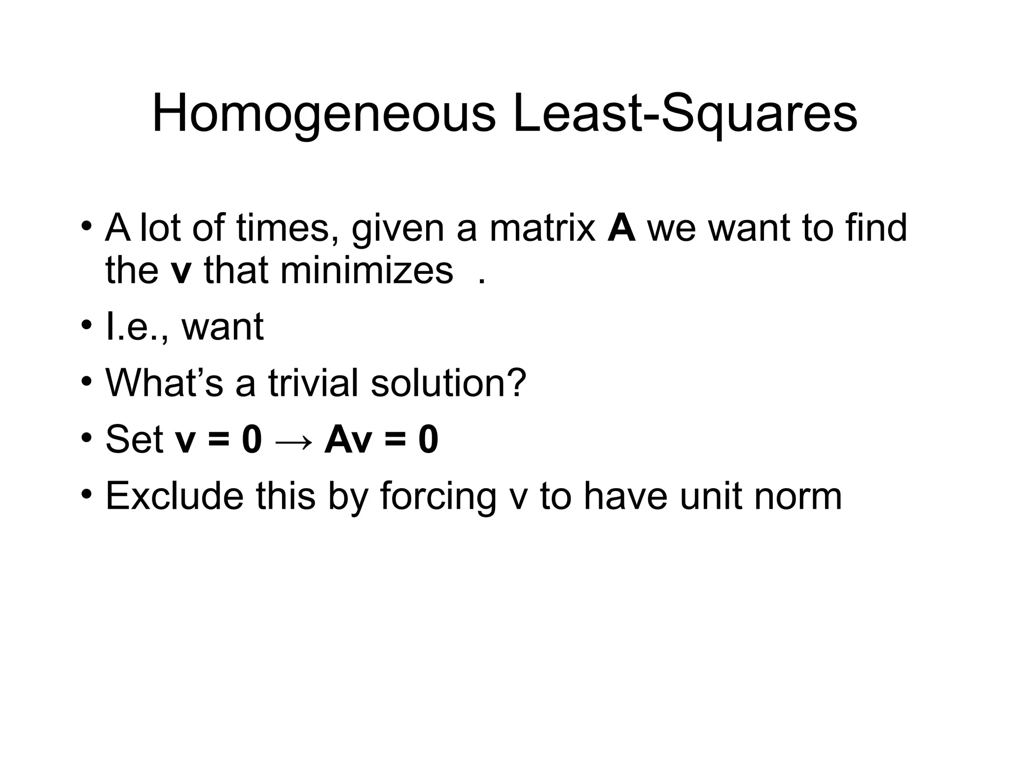
![Homogeneous Least-Squares
Given a set of unit vectors (aka directions) and I
want vector that is as orthogonal to all the as
possible (for some definition of orthogonal)
𝑨𝒗=
[− 𝒙𝟏
𝑻
−
¿⋮ ¿− ¿
−¿
]𝒗
Stack into A, compute Av
¿
[
𝒙𝟏
𝑻
𝒗
⋮
𝒙𝒏
𝑻
𝒗]
𝒙𝟏
𝒙𝟐
𝒙𝒏
…
𝒗
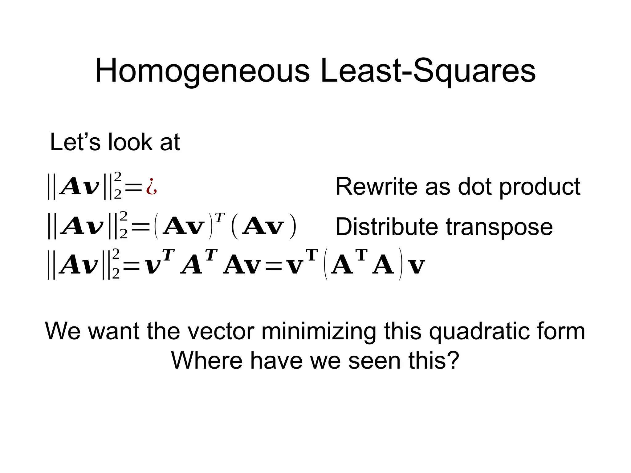
‖𝑨𝒗‖
𝟐
=∑
𝒊
𝒏
(𝒙𝒊
𝑻
𝒗 )
𝟐
Compute
0 if
orthog
Sum of how orthog. v is to each x](https://image.slidesharecdn.com/04math-241123011744-b40b74c3/75/Numerical-Linear-Algebra-in-digital-image-processing-101-2048.jpg)


![Vectors
[2,3] = + 3 x [0,1]
2 x [1,0]
2 x + 3 x
e1 e2
2 x + 3 x
x = [2,3] Can be arbitrary # of
dimensions
(typically denoted Rn
)](https://crownmelresort.com/image.slidesharecdn.com/04math-241123011744-b40b74c3/75/Numerical-Linear-Algebra-in-digital-image-processing-26-2048.jpg)
![Vectors
x = [2,3]
𝒙 =
[2
3]
𝒙1=2
𝒙2=3
Just an array!
Get in the habit of thinking of
them as columns.](https://crownmelresort.com/image.slidesharecdn.com/04math-241123011744-b40b74c3/75/Numerical-Linear-Algebra-in-digital-image-processing-27-2048.jpg)
![Scaling Vectors
x = [2,3]
2x = [4,6] • Can scale vector by a scalar
• Scalar = single number
• Dimensions changed
independently
• Changes magnitude / length,
does not change direction.](https://crownmelresort.com/image.slidesharecdn.com/04math-241123011744-b40b74c3/75/Numerical-Linear-Algebra-in-digital-image-processing-28-2048.jpg)
![Adding Vectors
y = [3,1]
x+y = [5,4]
x = [2,3]
• Can add vectors
• Dimensions changed independently
• Order irrelevant
• Can change direction and magnitude](https://crownmelresort.com/image.slidesharecdn.com/04math-241123011744-b40b74c3/75/Numerical-Linear-Algebra-in-digital-image-processing-29-2048.jpg)
![Scaling and Adding
y = [3,1]
2x+y = [7,7]
Can do both at the same
time
x = [2,3]](https://crownmelresort.com/image.slidesharecdn.com/04math-241123011744-b40b74c3/75/Numerical-Linear-Algebra-in-digital-image-processing-30-2048.jpg)
![Measuring Length
y = [3,1]
x = [2,3]
Magnitude / length / (L2) norm of vector
‖𝒙‖=‖𝒙‖2=
(∑
𝑖
𝑛
𝑥𝑖
2
)
1/2
There are other norms; assume L2
unless told otherwise
‖𝒙‖2=√13
‖𝒚‖2 =√10
Why?](https://crownmelresort.com/image.slidesharecdn.com/04math-241123011744-b40b74c3/75/Numerical-Linear-Algebra-in-digital-image-processing-31-2048.jpg)
![Normalizing a Vector
x = [2,3]
y = [3,1]
𝒙′
=𝒙 /‖𝒙‖𝟐
𝒚′
= 𝒚 /‖𝒚‖𝟐
Diving by norm gives
something on the unit
sphere (all vectors with
length 1)](https://crownmelresort.com/image.slidesharecdn.com/04math-241123011744-b40b74c3/75/Numerical-Linear-Algebra-in-digital-image-processing-32-2048.jpg)

![Dot Products
𝒆𝟏
𝒆𝟐
𝒙⋅𝒚 =∑
𝑖
𝑛
𝑥𝑖 𝑦𝑖
𝒙=[2,3]
What’s , ?
Ans: ;
• Dot product is projection
• Amount of x that’s also
pointing in direction of y](https://crownmelresort.com/image.slidesharecdn.com/04math-241123011744-b40b74c3/75/Numerical-Linear-Algebra-in-digital-image-processing-34-2048.jpg)
![Dot Products
What’s ?
Ans:
𝒙⋅𝒚 =∑
𝑖
𝑛
𝑥𝑖 𝑦𝑖
𝒙=[2,3]](https://crownmelresort.com/image.slidesharecdn.com/04math-241123011744-b40b74c3/75/Numerical-Linear-Algebra-in-digital-image-processing-35-2048.jpg)
![Special Angles
𝒙′
𝒚′
𝜃
[1
0 ]⋅[0
1 ]=0 ∗1+ 1∗ 0=0
Perpendicular /
orthogonal vectors
have dot product 0
irrespective of their
magnitude
𝒙
𝒚](https://crownmelresort.com/image.slidesharecdn.com/04math-241123011744-b40b74c3/75/Numerical-Linear-Algebra-in-digital-image-processing-36-2048.jpg)
![Special Angles
[𝑥1
𝑥2
]⋅
[𝑦1
𝑦2
]=𝑥1 𝑦 1+ 𝑥2 𝑦2=0
Perpendicular /
orthogonal vectors
have dot product 0
irrespective of their
magnitude
𝒙′
𝒚′
𝜃
𝒙
𝒚](https://crownmelresort.com/image.slidesharecdn.com/04math-241123011744-b40b74c3/75/Numerical-Linear-Algebra-in-digital-image-processing-37-2048.jpg)
![Orthogonal Vectors
𝒙=[2,3]
• Geometrically,
what’s the set of
vectors that are
orthogonal to x?
• A line [3,-2]](https://crownmelresort.com/image.slidesharecdn.com/04math-241123011744-b40b74c3/75/Numerical-Linear-Algebra-in-digital-image-processing-38-2048.jpg)
![Orthogonal Vectors
• What’s the set of vectors that are
orthogonal to x = [5,0,0]?
• A plane/2D space of vectors/any
vector
• What’s the set of vectors that are
orthogonal to x and y = [0,5,0]?
• A line/1D space of vectors/any
vector
• Ambiguity in sign and magnitude
𝒙
𝒙
𝒚](https://crownmelresort.com/image.slidesharecdn.com/04math-241123011744-b40b74c3/75/Numerical-Linear-Algebra-in-digital-image-processing-39-2048.jpg)


![Matrices
Horizontally concatenate n, m-dim column vectors
and you get a mxn matrix A (here 2x3)
𝑨=[ 𝒗1 ,⋯ , 𝒗 𝑛]=
[𝑣11
𝑣21
𝑣31
𝑣12
𝑣22
𝑣32
]
a
(scalar)
lowercase
undecorated
a
(vector)
lowercase
bold or arrow
A
(matrix)
uppercase
bold](https://crownmelresort.com/image.slidesharecdn.com/04math-241123011744-b40b74c3/75/Numerical-Linear-Algebra-in-digital-image-processing-42-2048.jpg)
![Matrices
Vertically concatenate m, n-dim row vectors
and you get a mxn matrix A (here 2x3)
𝐴=
[
𝒖1
𝑇
⋮
𝒖𝑛
𝑇 ]=
[𝑢11
𝑢12
𝑢13
𝑢21
𝑢22
𝑢23
]
Transpose: flip
rows / columns [
𝑎
𝑏
𝑐 ]
𝑇
=[𝑎 𝑏 𝑐 ] (3x1)T
= 1x3](https://crownmelresort.com/image.slidesharecdn.com/04math-241123011744-b40b74c3/75/Numerical-Linear-Algebra-in-digital-image-processing-43-2048.jpg)
![Matrix-Vector Product
𝒚2 𝑥1= 𝑨2 𝑥3 𝒙3 𝑥 1
𝒚 =𝑥1 𝒗𝟏 +𝑥2 𝒗𝟐 +𝑥3 𝒗𝟑
Linear combination of columns of A
[𝑦1
𝑦2
]=¿[𝒗𝟏 𝒗𝟐 𝒗𝟑 ][
𝑥1
𝑥2
𝑥3
]](https://crownmelresort.com/image.slidesharecdn.com/04math-241123011744-b40b74c3/75/Numerical-Linear-Algebra-in-digital-image-processing-44-2048.jpg)
![Matrix-Vector Product
𝒚2 𝑥1= 𝑨2 𝑥3 𝒙3 𝑥 1
𝑦 1=𝒖𝟏
𝑻
𝒙
Dot product between rows of A and x
𝑦 2=𝒖𝟐
𝑻
𝒙
[𝒖𝟏
𝑻
𝒖𝟐
𝑻
]
[𝑦1
𝑦2
]=¿ 𝒙
3
3](https://crownmelresort.com/image.slidesharecdn.com/04math-241123011744-b40b74c3/75/Numerical-Linear-Algebra-in-digital-image-processing-45-2048.jpg)
![Matrix Multiplication
[− 𝒂𝟏
𝑻
−
¿⋮ ¿− ¿
−¿
]¿
𝑨𝑩=¿
Generally: Amn and Bnp yield product (AB)mp
Yes – in A, I’m referring to the rows, and in B,
I’m referring to the columns](https://crownmelresort.com/image.slidesharecdn.com/04math-241123011744-b40b74c3/75/Numerical-Linear-Algebra-in-digital-image-processing-46-2048.jpg)
![Matrix Multiplication
[− 𝒂𝟏
𝑻
−
¿⋮ ¿− ¿
−¿
]
¿
𝑨𝑩=¿
[
𝒂𝟏
𝑻
𝒃𝟏 ⋯ 𝒂𝟏
𝑻
𝒃𝒑
⋮ ⋱ ⋮
𝒂𝒎
𝑻
𝒃𝟏 ⋯ 𝒂𝒎
𝑻
𝒃𝒑
]
𝑨 𝑩𝑖𝑗=𝒂𝒊
𝑻
𝒃𝒋
Generally: Amn and Bnp yield product (AB)mp](https://crownmelresort.com/image.slidesharecdn.com/04math-241123011744-b40b74c3/75/Numerical-Linear-Algebra-in-digital-image-processing-47-2048.jpg)

![Operations They Don’t Teach
[𝑎+𝑒 𝑏+𝑒
𝑐 +𝑒 𝑑+𝑒]
[𝑎 𝑏
𝑐 𝑑]+
[𝑒 𝑓
𝑔 h]=¿
[𝑎+𝑒 𝑏+ 𝑓
𝑐+𝑔 𝑑+h ]
You Probably Saw Matrix Addition
[𝑎 𝑏
𝑐 𝑑]+𝑒=¿
What is this? FYI: e is a scalar](https://crownmelresort.com/image.slidesharecdn.com/04math-241123011744-b40b74c3/75/Numerical-Linear-Algebra-in-digital-image-processing-49-2048.jpg)
![Broadcasting
[𝑎 𝑏
𝑐 𝑑]+𝑒
¿
[𝑎 𝑏
𝑐 𝑑 ]+
[𝑒 𝑒
𝑒 𝑒]
¿
[𝑎 𝑏
𝑐 𝑑 ]+𝟏2 𝑥 2 𝑒
If you want to be pedantic and proper, you expand
e by multiplying a matrix of 1s (denoted 1)
Many smart matrix libraries do this automatically.
This is the source of many bugs.](https://crownmelresort.com/image.slidesharecdn.com/04math-241123011744-b40b74c3/75/Numerical-Linear-Algebra-in-digital-image-processing-50-2048.jpg)
![Broadcasting Example
𝑷 =
[
𝑥1 𝑦1
⋮ ⋮
𝑥𝑛 𝑦𝑛
] 𝒗 =
[𝑎
𝑏]
Given: a nx2 matrix P and a 2D column vector v,
Want: nx2 difference matrix D
𝑫=
[
𝑥1 − 𝑎 𝑦1 − 𝑏
⋮ ⋮
𝑥𝑛 − 𝑎 𝑦𝑛 − 𝑏]
𝑷 −𝒗𝑇
=¿
[
𝑥1 𝑦1
⋮ ⋮
𝑥𝑛 𝑦𝑛
]−
[𝑎 𝑏]
[𝑎 𝑏]
⋮
Blue stuff is
assumed /
broadcast](https://crownmelresort.com/image.slidesharecdn.com/04math-241123011744-b40b74c3/75/Numerical-Linear-Algebra-in-digital-image-processing-51-2048.jpg)


![Implementation
imNew = im**4
Python+Numpy (right way):
Python+Numpy (slow way – why? ):
imNew = np.zeros(im.shape)
for y in range(im.shape[0]):
for x in range(im.shape[1]):
imNew[y,x] = im[y,x]**expFactor](https://crownmelresort.com/image.slidesharecdn.com/04math-241123011744-b40b74c3/75/Numerical-Linear-Algebra-in-digital-image-processing-56-2048.jpg)


![Implementation
imNew = im**4
Python+Numpy (right way):
Python+Numpy (slow way – why? ):
imNew = np.zeros(im.shape)
for y in range(im.shape[0]):
for x in range(im.shape[1]):
imNew[y,x] = im[y,x]**expFactor](https://crownmelresort.com/image.slidesharecdn.com/04math-241123011744-b40b74c3/75/Numerical-Linear-Algebra-in-digital-image-processing-60-2048.jpg)

![Sums Across Axes
𝑨=
[
𝑥1 𝑦1
⋮ ⋮
𝑥𝑛 𝑦𝑛
]
Suppose have
Nx2 matrix A
Σ( 𝑨 ,1)=
[
𝑥1 +𝑦1
⋮
𝑥𝑛 +𝑦𝑛
]
ND col. vec.
Σ( 𝑨 ,0)=
[∑
𝑖=1
𝑛
𝑥𝑖 ,∑
𝑖=1
𝑛
𝑦𝑖
]
2D row vec
Note – libraries distinguish between N-D column vector and Nx1 matrix.](https://crownmelresort.com/image.slidesharecdn.com/04math-241123011744-b40b74c3/75/Numerical-Linear-Algebra-in-digital-image-processing-62-2048.jpg)

![Vectorizing Example
𝑿=
[− 𝒙1 −
¿⋮ ¿− ¿
−¿]𝒀=
[− 𝒚1 −
¿⋮ ¿− ¿
−¿]
(𝑿 𝒀𝑻
)𝑖𝑗=𝒙𝒊
𝑻
𝒚 𝒋
𝒀 𝑻
=¿
𝚺( 𝑿
𝟐
,𝟏)=
[
‖𝒙𝟏‖
𝟐
⋮
‖𝒙𝑵‖
𝟐 ]
Compute a Nx1
vector of norms
(can also do Mx1)
Compute a NxM
matrix of dot products](https://crownmelresort.com/image.slidesharecdn.com/04math-241123011744-b40b74c3/75/Numerical-Linear-Algebra-in-digital-image-processing-64-2048.jpg)
![Vectorizing Example
𝐃=(Σ(𝑿
𝟐
,1)+Σ(𝒀
𝟐
,1)
𝑻
−2 𝑿𝒀
𝑻
)
1/2
[
‖𝒙𝟏‖
𝟐
⋮
‖𝒙 𝑵‖
𝟐 ]+[‖𝒚 1‖
𝟐
⋯ ‖𝒚 𝑀‖
𝟐
]
(Σ( 𝑿
2
, 1)+Σ (𝒀
2
,1)
𝑇
)𝑖𝑗=‖𝒙𝑖‖
2
+‖𝒚 𝑗‖
2
[
‖𝒙𝟏‖
2
+‖𝒚 𝟏‖
2
⋯ ‖𝒙𝟏‖
2
+‖𝒚 𝑴‖
2
⋮ ⋱ ⋮
‖𝒙 𝑵‖
2
+‖𝒚 𝟏‖
2
⋯ ‖𝒙 𝑵‖
2
+‖𝒚 𝑴‖
2 ] Why?](https://crownmelresort.com/image.slidesharecdn.com/04math-241123011744-b40b74c3/75/Numerical-Linear-Algebra-in-digital-image-processing-65-2048.jpg)


![Linear Independence
𝒚 =
[
0
− 2
1 ]=¿
1
2
𝒂−
1
3
𝒃
𝒙 =
[
0
0
4 ]=¿
2𝒂
• Is the set {a,b,c} linearly independent?
• Is the set {a,b,x} linearly independent?
• Max # of independent 3D vectors?
𝒂=
[
0
0
2 ]𝒃=
[
0
6
0]𝒄=
[
5
0
0]
Suppose:
A set of vectors is linearly independent if you can’t
write one as a linear combination of the others.](https://crownmelresort.com/image.slidesharecdn.com/04math-241123011744-b40b74c3/75/Numerical-Linear-Algebra-in-digital-image-processing-68-2048.jpg)
![Span
Span: all linear
combinations of a
set of vectors
Span({ }) =
Span({[0,2]}) = ?
All vertical lines
through origin =
Is blue in {red}’s
span?](https://crownmelresort.com/image.slidesharecdn.com/04math-241123011744-b40b74c3/75/Numerical-Linear-Algebra-in-digital-image-processing-69-2048.jpg)


![An Intuition
x
Ax
y1
y2
y3
x1 x2 x3
y
𝒚 = 𝑨𝒙=
[
¿ ¿ ¿
𝒄𝟏 𝒄𝟐 𝒄𝒏
¿ ¿ ¿
][
𝑥1
𝑥2
𝑥3
]
x – knobs on machine (e.g., fuel, brakes)
y – state of the world (e.g., where you are)
A – machine (e.g., your car)](https://crownmelresort.com/image.slidesharecdn.com/04math-241123011744-b40b74c3/75/Numerical-Linear-Algebra-in-digital-image-processing-73-2048.jpg)
![Linear Independence
𝒚 = 𝑨𝒙=
[
¿ ¿ ¿
𝒄𝟏 𝛼 𝒄𝟏 𝒄𝟐
¿ ¿ ¿
][
𝑥1
𝑥2
𝑥3
]
Suppose the columns of 3x3 matrix A are not
linearly independent (c1, αc1, c2 for instance)
𝒚 =𝑥1 𝒄𝟏+𝛼 𝑥2 𝒄𝟏+𝑥3 𝒄𝟐
𝒚 =(𝑥1+𝛼 𝑥2)𝒄𝟏+𝑥3 𝒄𝟐](https://crownmelresort.com/image.slidesharecdn.com/04math-241123011744-b40b74c3/75/Numerical-Linear-Algebra-in-digital-image-processing-74-2048.jpg)

![Linear Independence
𝑨𝒙 =( 𝑥1 + 𝛼 𝑥 2 ) 𝒄 𝟏+ 𝑥 3 𝒄𝟐
• Or, given a vector y there’s not a unique
vector x s.t. y =Ax
• Not all y have a corresponding x s.t. y=Ax
𝒚 = 𝑨
[
𝑥1+ 𝛽
𝑥2 − 𝛽 /𝛼
𝑥3
]
• Can write y an infinite number of ways by
adding to x1 and subtracting from x2
Recall:
¿(𝑥1+ 𝛽+𝛼 𝑥2− 𝛼
𝛽
𝛼 )𝑐1+𝑥3 𝑐2](https://crownmelresort.com/image.slidesharecdn.com/04math-241123011744-b40b74c3/75/Numerical-Linear-Algebra-in-digital-image-processing-76-2048.jpg)
![Linear Independence
𝑨𝒙 =( 𝑥1 + 𝛼 𝑥 2 ) 𝒄 𝟏+ 𝑥 3 𝒄𝟐
• An infinite number of non-zero vectors x can
map to a zero-vector y
• Called the right null-space of A.
𝒚 = 𝑨
[
𝛽
− 𝛽 / 𝛼
0 ]
¿(𝛽− 𝛼
𝛽
𝛼)𝒄𝟏+0𝒄𝟐
• What else can we cancel out?](https://crownmelresort.com/image.slidesharecdn.com/04math-241123011744-b40b74c3/75/Numerical-Linear-Algebra-in-digital-image-processing-77-2048.jpg)


![Symmetric Matrices
• Symmetric: or
• Have lots of special
properties [
𝑎11 𝑎12 𝑎13
𝑎21 𝑎22 𝑎23
𝑎31 𝑎32 𝑎33
]
Any matrix of the form is symmetric.
Quick check: 𝑨
𝑻
=(𝑿
𝑻
𝑿)𝑻
𝑨
𝑻
=𝑿
𝑻
(𝑿
𝑻
)𝑻
𝑨𝑻
=𝑿𝑻
𝑿](https://crownmelresort.com/image.slidesharecdn.com/04math-241123011744-b40b74c3/75/Numerical-Linear-Algebra-in-digital-image-processing-80-2048.jpg)
![Special Matrices – Rotations
[
𝑟1 1 𝑟12 𝑟 13
𝑟 21 𝑟22 𝑟 23
𝑟 31 𝑟32 𝑟 33
]
• Rotation matrices rotate vectors and do not
change vector L2 norms ()
• Every row/column is unit norm
• Every row is linearly independent
• Transpose is inverse
• Determinant is 1 (otherwise it’s also a coordinate
flip/reflection), eigenvalues are 1](https://crownmelresort.com/image.slidesharecdn.com/04math-241123011744-b40b74c3/75/Numerical-Linear-Algebra-in-digital-image-processing-81-2048.jpg)


![Red box – unit square, Blue box – after f(x) = Ax.
What are the yellow lines and why?
𝑨=¿
[1.1 0
0 1.1]](https://crownmelresort.com/image.slidesharecdn.com/04math-241123011744-b40b74c3/75/Numerical-Linear-Algebra-in-digital-image-processing-85-2048.jpg)
![𝑨=¿
[0 .8 0
0 1.25]
Now I apply f(x) = Ax to these points
Pointy-end: Ax . Non-Pointy-End: x](https://crownmelresort.com/image.slidesharecdn.com/04math-241123011744-b40b74c3/75/Numerical-Linear-Algebra-in-digital-image-processing-86-2048.jpg)
![Red box – unit square, Blue box – after f(x) = Ax.
What are the yellow lines and why?
𝑨=¿
[0 .8 0
0 1.25]](https://crownmelresort.com/image.slidesharecdn.com/04math-241123011744-b40b74c3/75/Numerical-Linear-Algebra-in-digital-image-processing-87-2048.jpg)
![Red box – unit square, Blue box – after f(x) = Ax.
Can we draw any yellow lines?
𝑨=¿
[c os (𝑡) − sin (𝑡)
sin (𝑡) cos (𝑡) ]](https://crownmelresort.com/image.slidesharecdn.com/04math-241123011744-b40b74c3/75/Numerical-Linear-Algebra-in-digital-image-processing-88-2048.jpg)


![Solving Least-Squares
Start with two points (xi,yi)
[𝑦1
𝑦2
]=
[𝑥1 1
𝑥2 1 ][𝑚
𝑏 ]
𝒚 =𝑨𝒗
[𝑦1
𝑦2
]=
[𝑚 𝑥1 +𝑏
𝑚 𝑥2 +𝑏 ]
We know how to solve this –
invert A and find v (i.e., (m,b)
that fits points)
(x1,y1)
(x2,y2)](https://crownmelresort.com/image.slidesharecdn.com/04math-241123011744-b40b74c3/75/Numerical-Linear-Algebra-in-digital-image-processing-95-2048.jpg)
![Solving Least-Squares
Start with two points (xi,yi)
[𝑦1
𝑦2
]=
[𝑥1 1
𝑥2 1 ][𝑚
𝑏 ]
𝒚 =𝑨𝒗
‖[𝑦1
𝑦 2
]−
[𝑚 𝑥1 +𝑏
𝑚 𝑥2+ 𝑏]‖
2
‖𝒚 − 𝑨𝒗‖
2
=¿
¿ ( 𝑦1 −(𝑚 𝑥1 +𝑏))
2
+( 𝑦2 − (𝑚 𝑥2 +𝑏))
2
(x1,y1)
(x2,y2)
The sum of squared differences between
the actual value of y and
what the model says y should be.](https://crownmelresort.com/image.slidesharecdn.com/04math-241123011744-b40b74c3/75/Numerical-Linear-Algebra-in-digital-image-processing-96-2048.jpg)
![Solving Least-Squares
Suppose there are n > 2 points
[
𝑦1
⋮
𝑦 𝑁
]=
[
𝑥1 1
⋮ ⋮
𝑥𝑁 1][𝑚
𝑏 ]
𝒚 =𝑨𝒗
Compute again
‖𝒚 − 𝑨𝒗‖
2
=∑
𝑖=1
𝑛
(𝑦𝑖 −(𝑚 𝑥𝑖+𝑏))
2](https://crownmelresort.com/image.slidesharecdn.com/04math-241123011744-b40b74c3/75/Numerical-Linear-Algebra-in-digital-image-processing-97-2048.jpg)


![Homogeneous Least-Squares
Given a set of unit vectors (aka directions) and I
want vector that is as orthogonal to all the as
possible (for some definition of orthogonal)
𝑨𝒗=
[− 𝒙𝟏
𝑻
−
¿⋮ ¿− ¿
−¿
]𝒗
Stack into A, compute Av
¿
[
𝒙𝟏
𝑻
𝒗
⋮
𝒙𝒏
𝑻
𝒗]
𝒙𝟏
𝒙𝟐
𝒙𝒏
…
𝒗
‖𝑨𝒗‖
𝟐
=∑
𝒊
𝒏
(𝒙𝒊
𝑻
𝒗 )
𝟐
Compute
0 if
orthog
Sum of how orthog. v is to each x](https://crownmelresort.com/image.slidesharecdn.com/04math-241123011744-b40b74c3/75/Numerical-Linear-Algebra-in-digital-image-processing-101-2048.jpg)


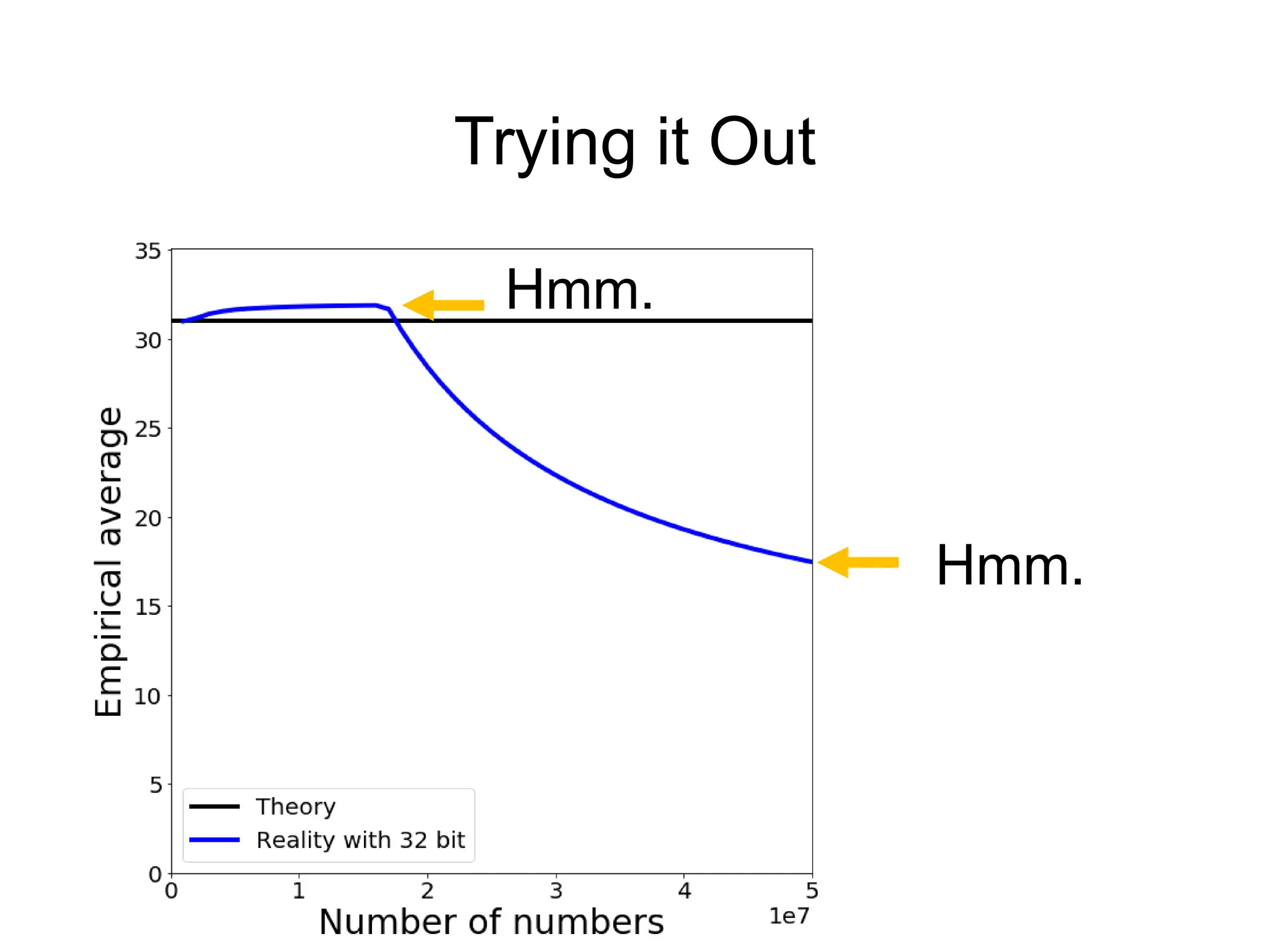
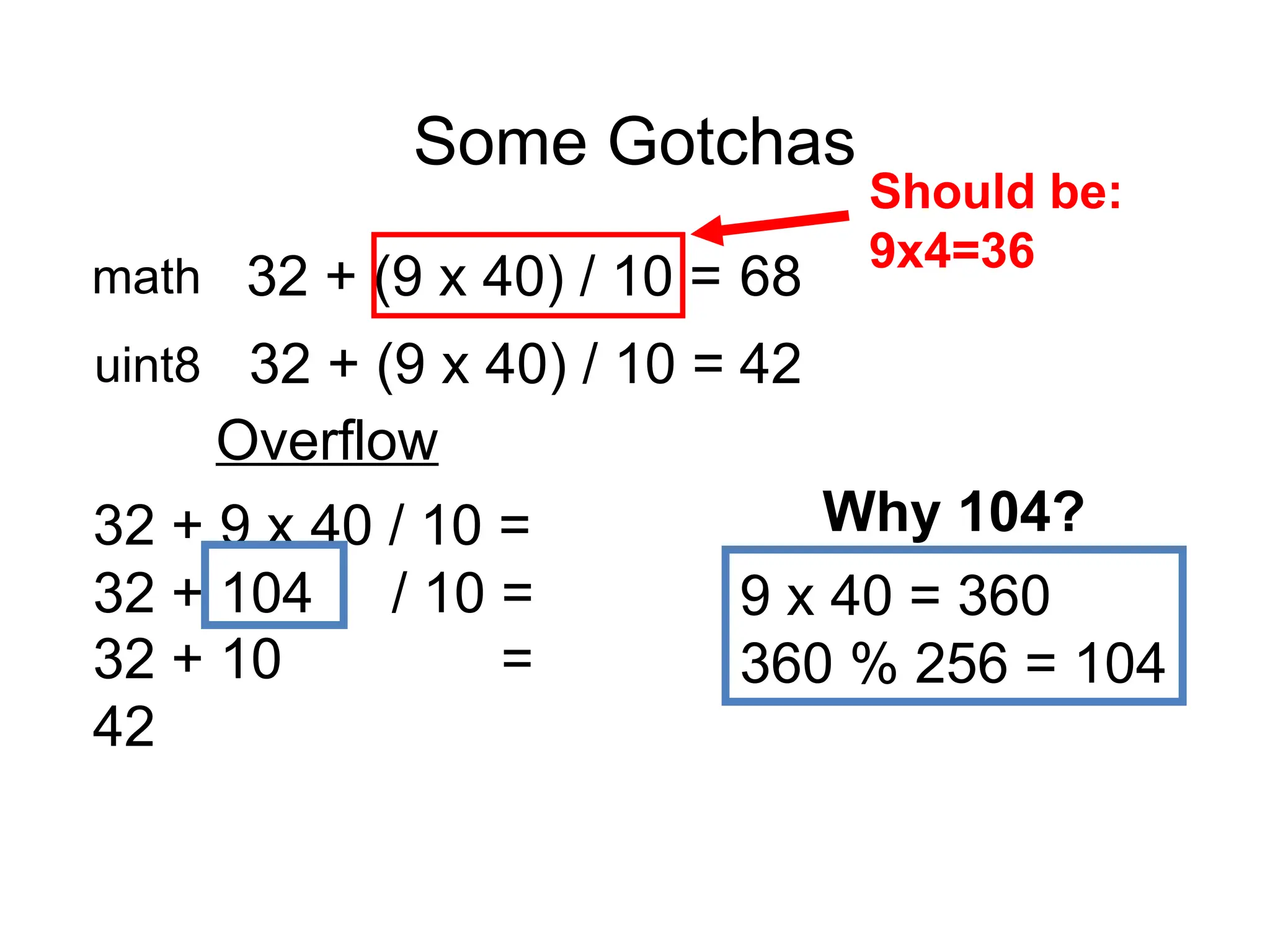
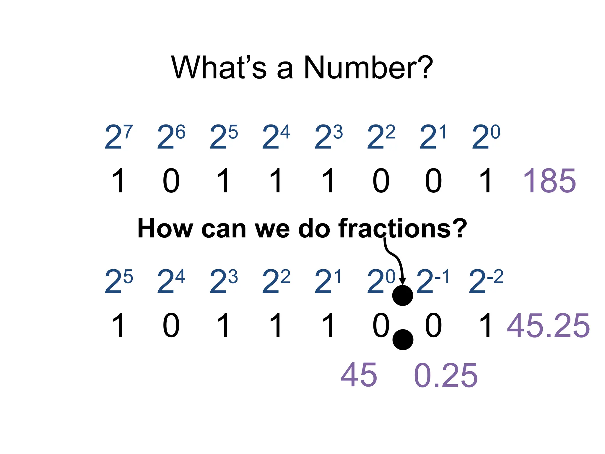
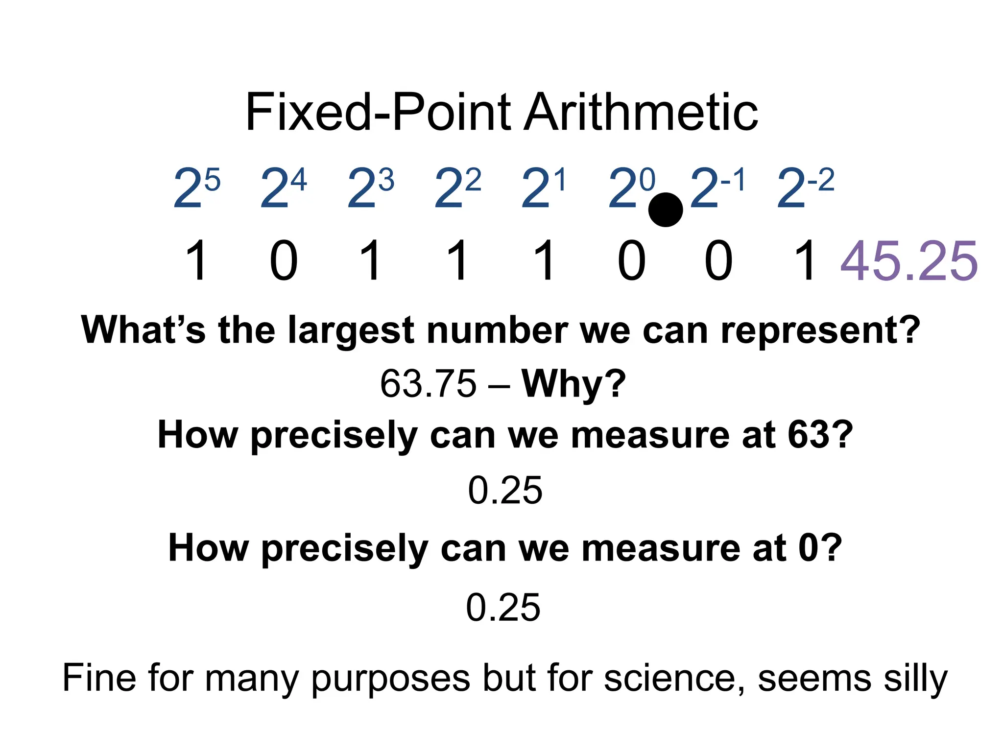
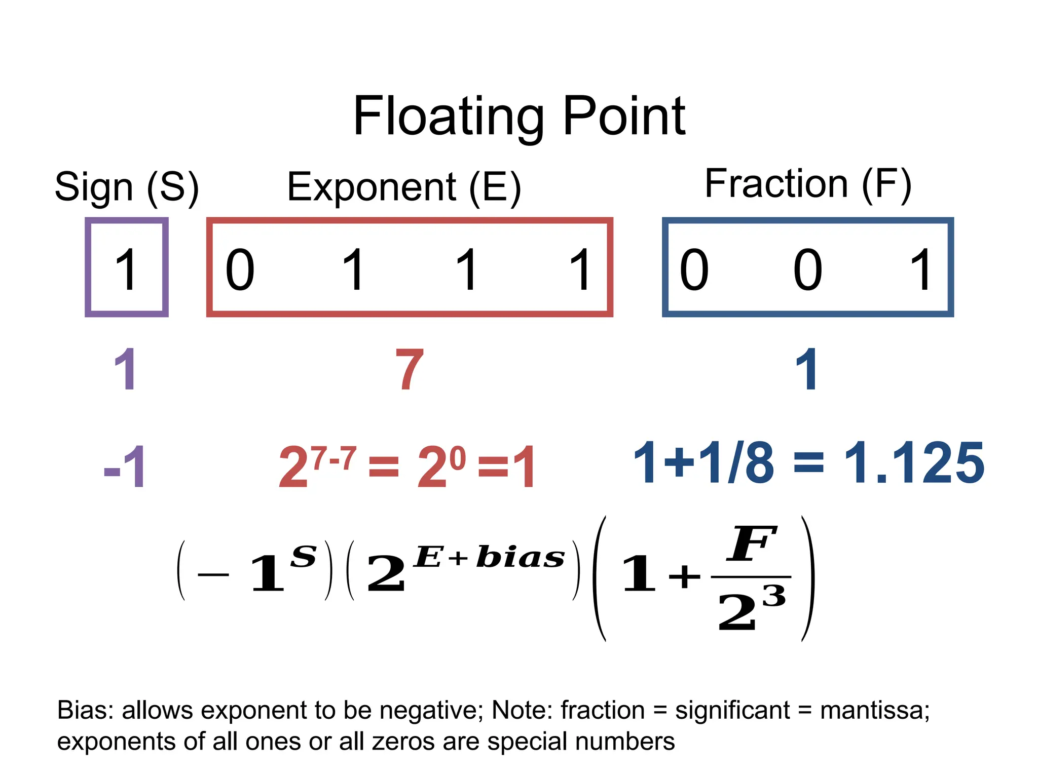
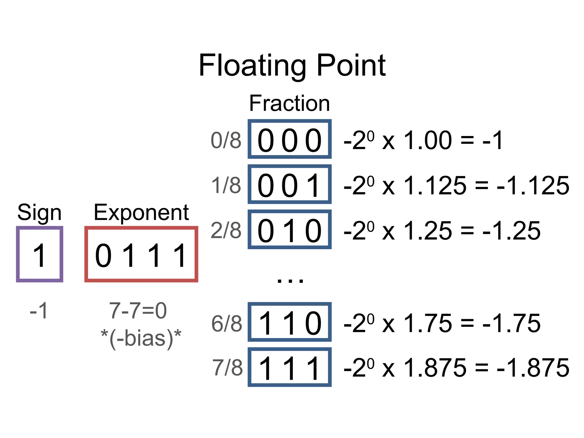
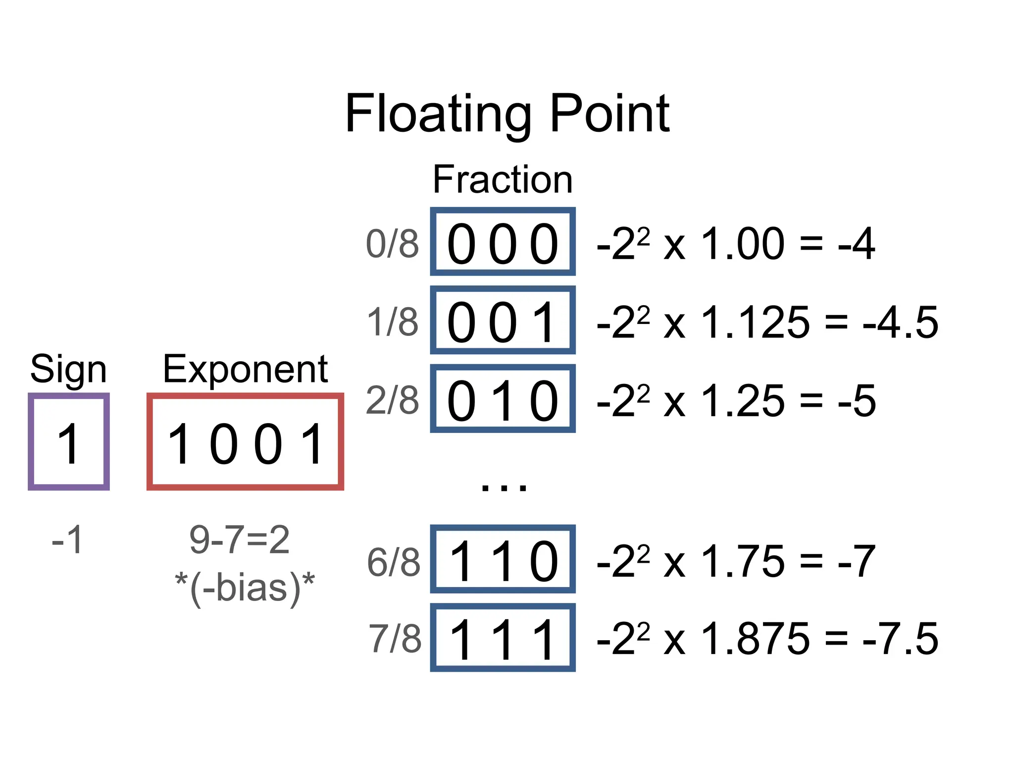
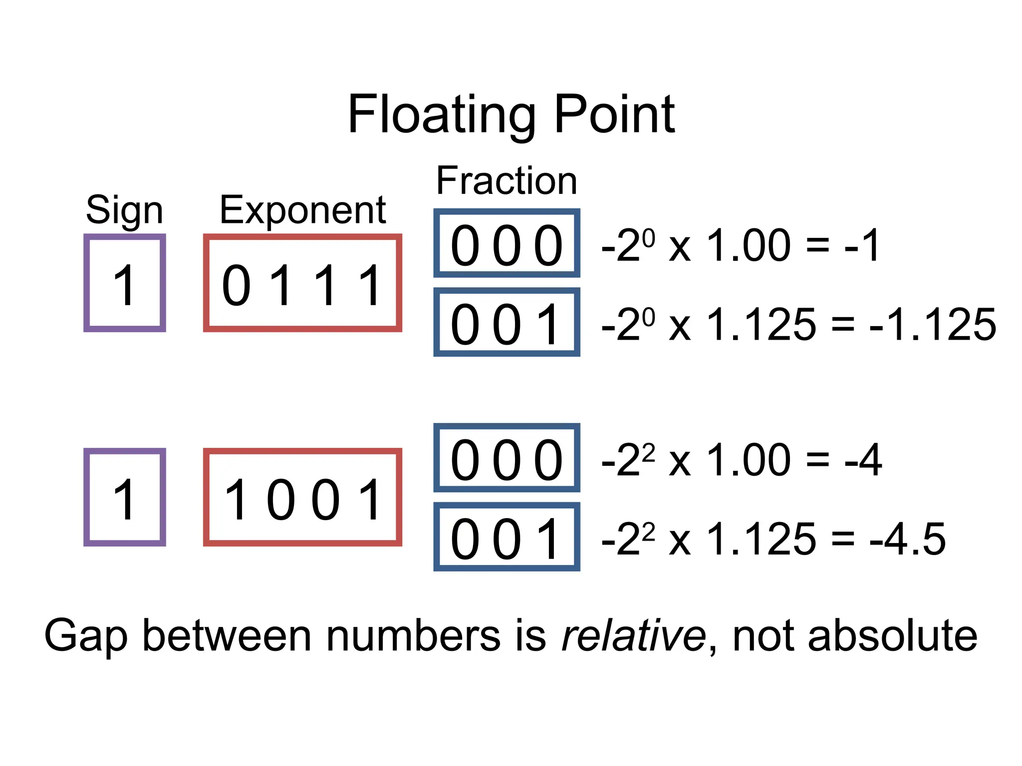
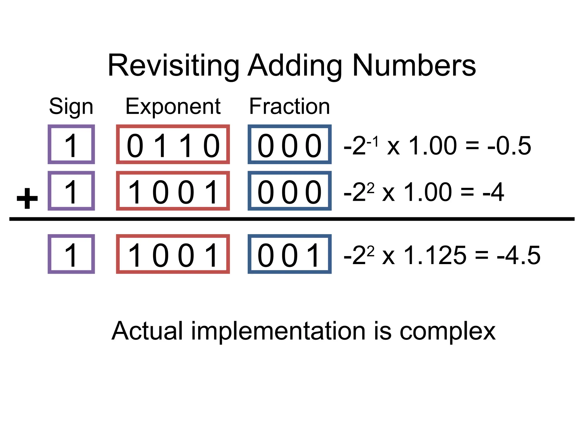
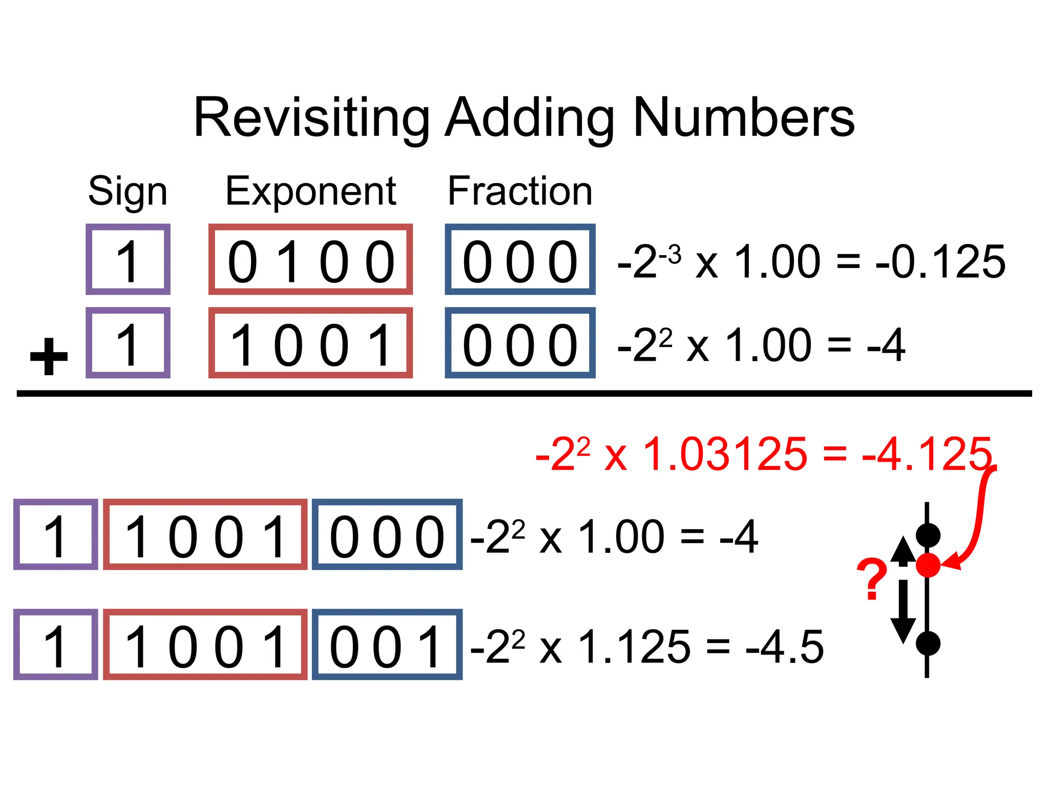
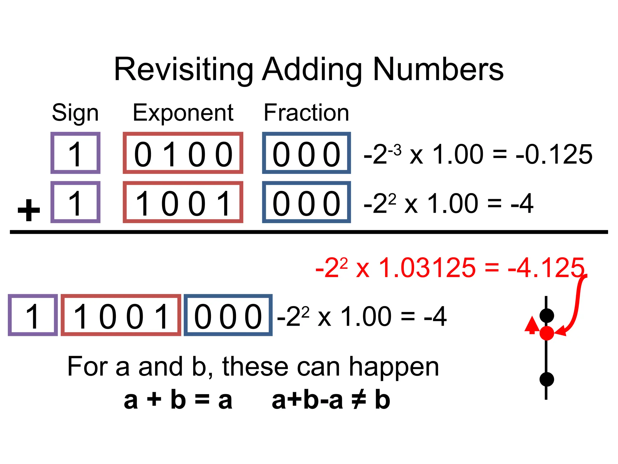
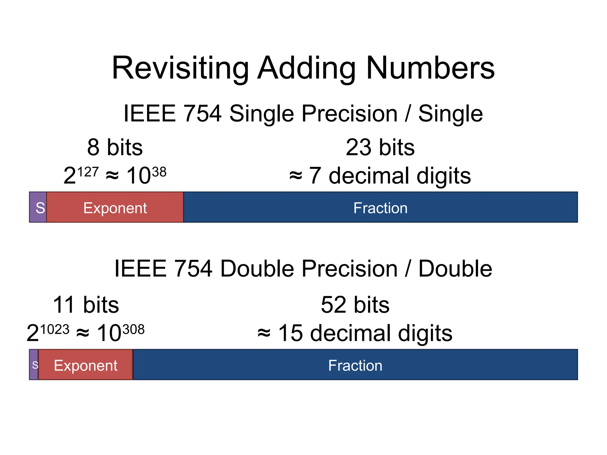
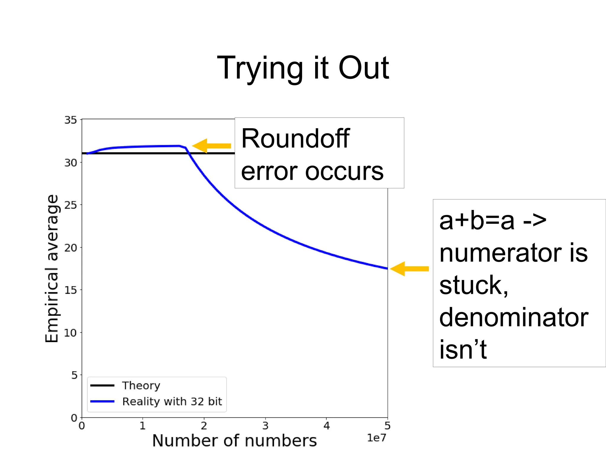
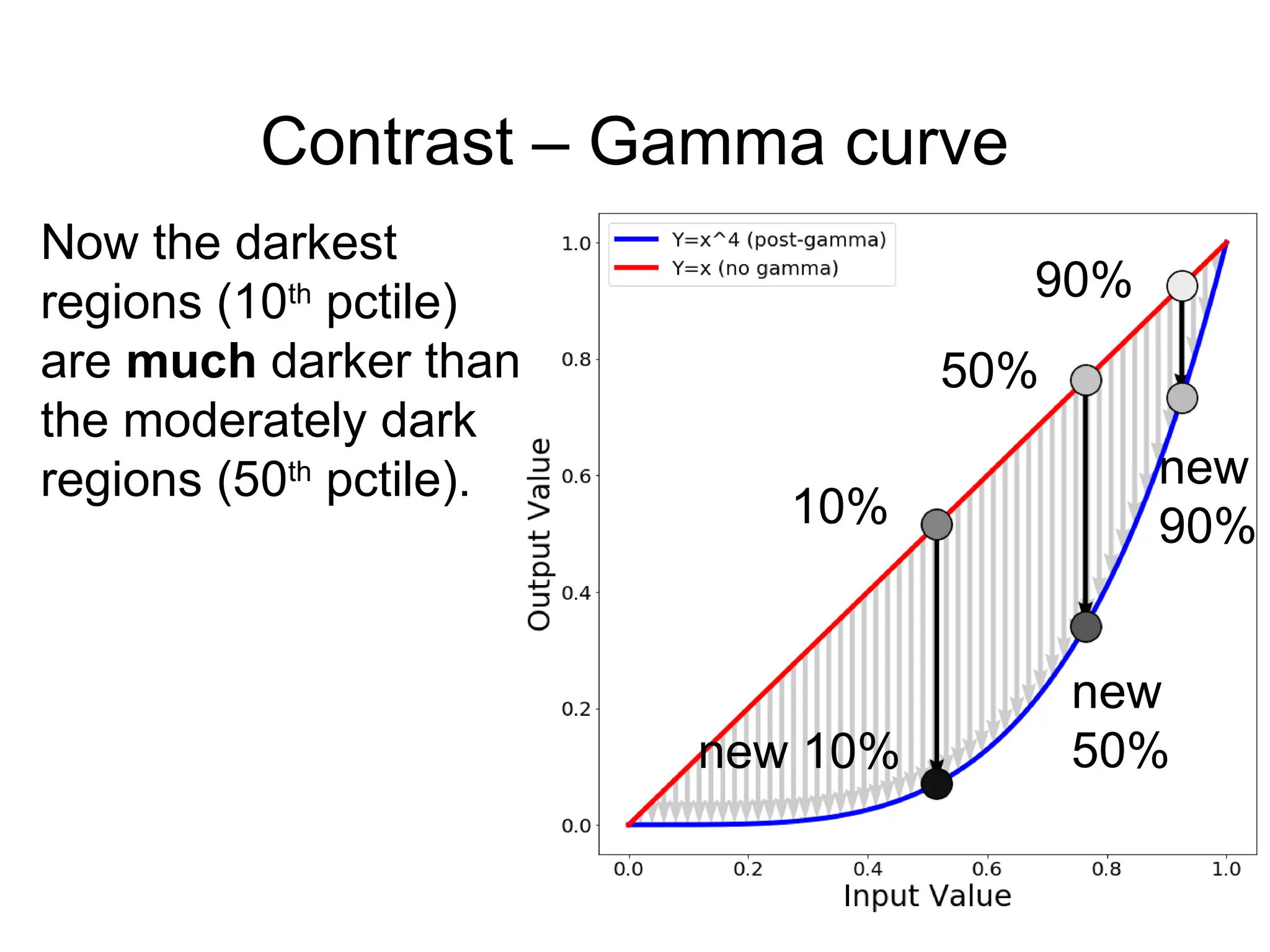
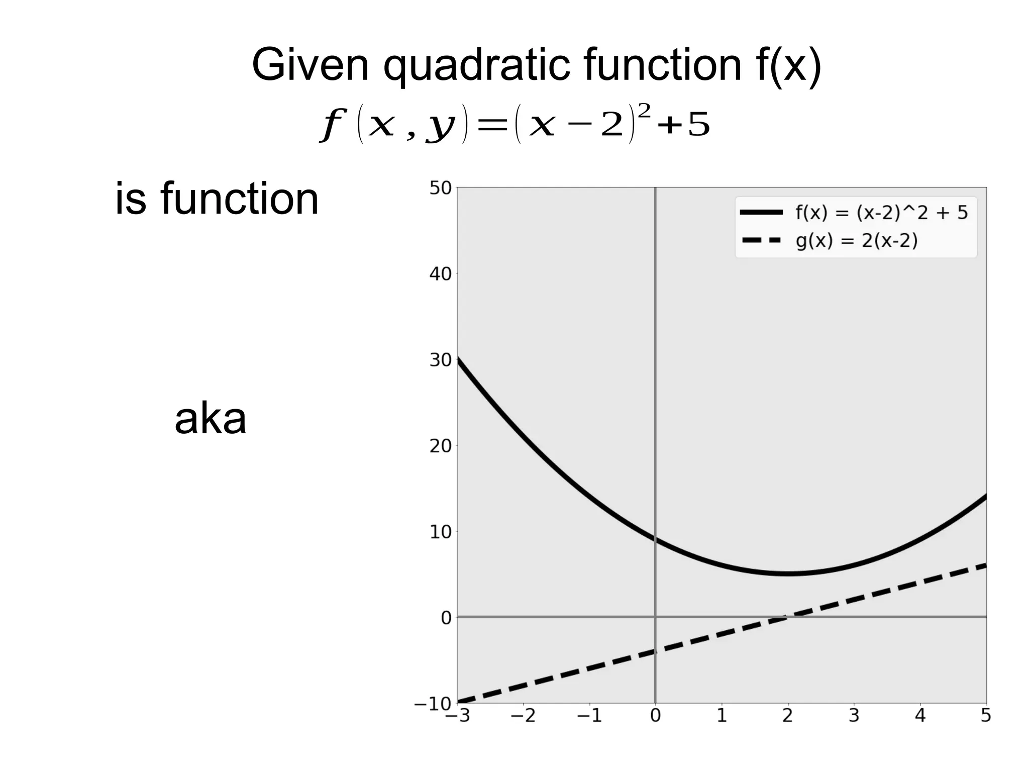
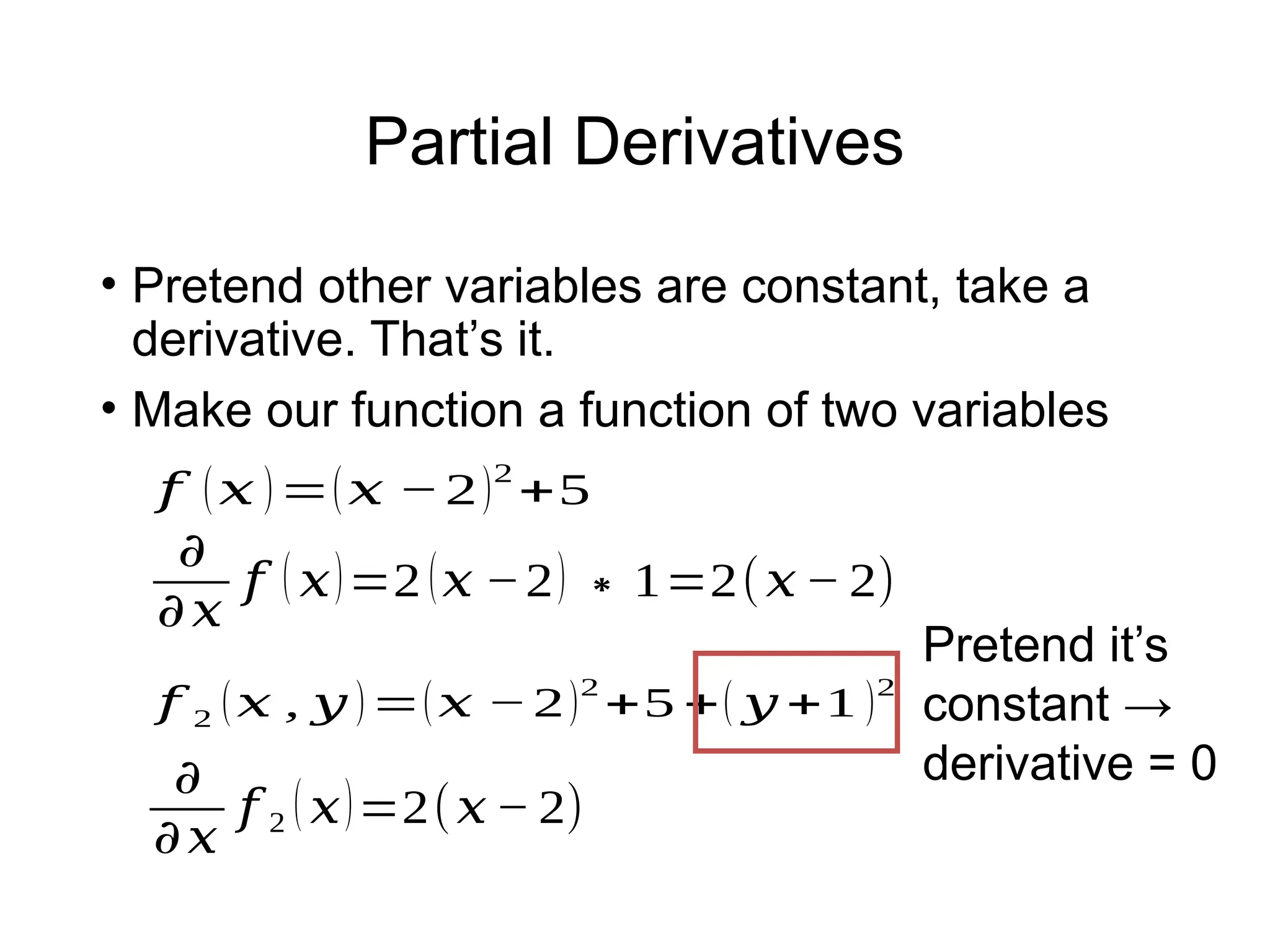
The document covers the topics for the Numerical Linear Algebra course (EECS 442) taught by David Fouhey at the University of Michigan during Fall 2019. It discusses administrative details, introduces key mathematical concepts, and emphasizes practical applications, including floating-point arithmetic, vectors, and matrices. The content aims to strengthen students' existing knowledge and addresses potential challenges in understanding numerical computations.