Downloaded 11 times
![Industrial Engineering Letters
ISSN 2224-6096 (Paper) ISSN 2225-0581 (online
Vol.3, No.7, 2013
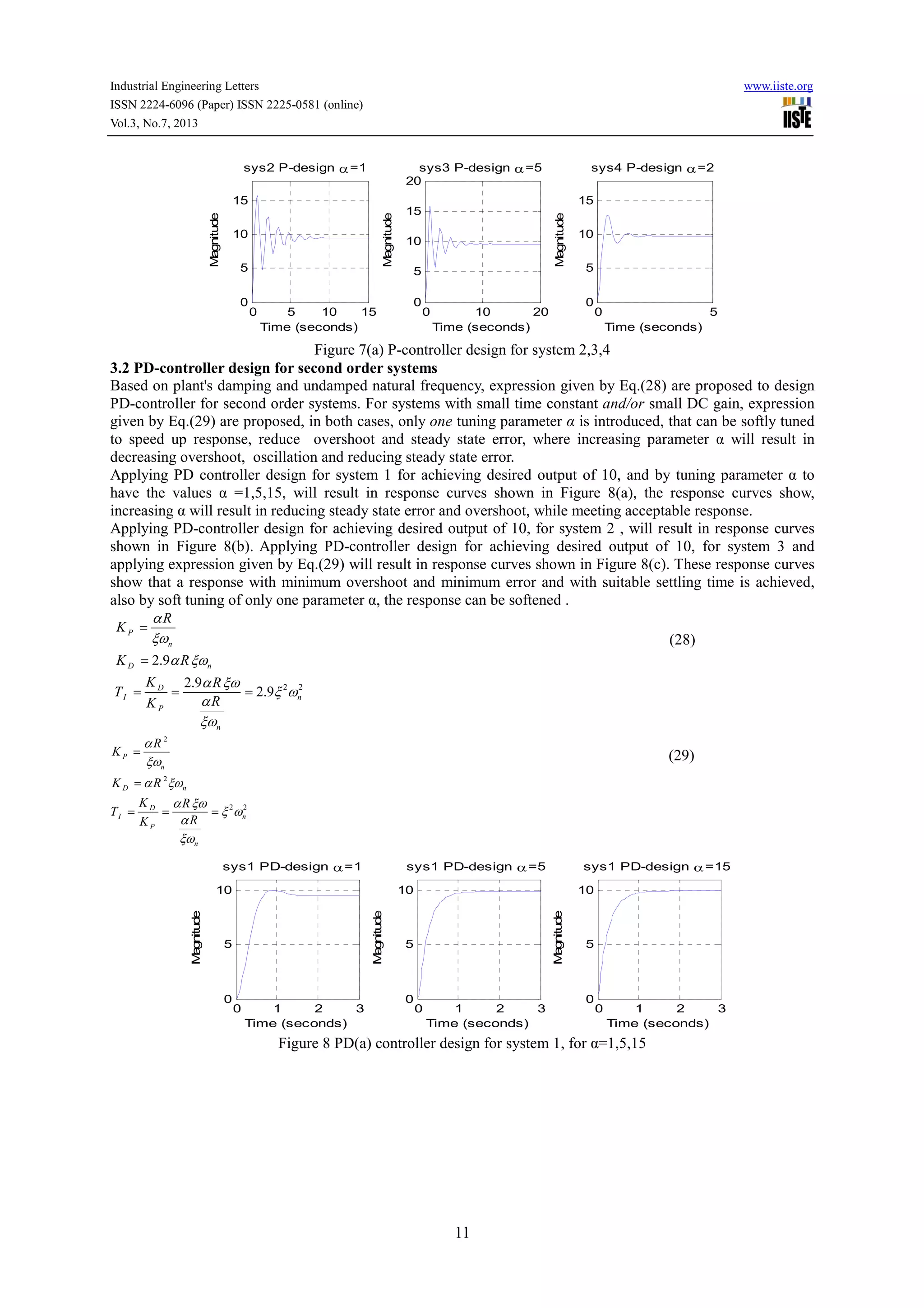
3.5 Summary: Controller design for second order systems
The proposed method for second order systems and expressions for controllers terms
summarized in Table 10
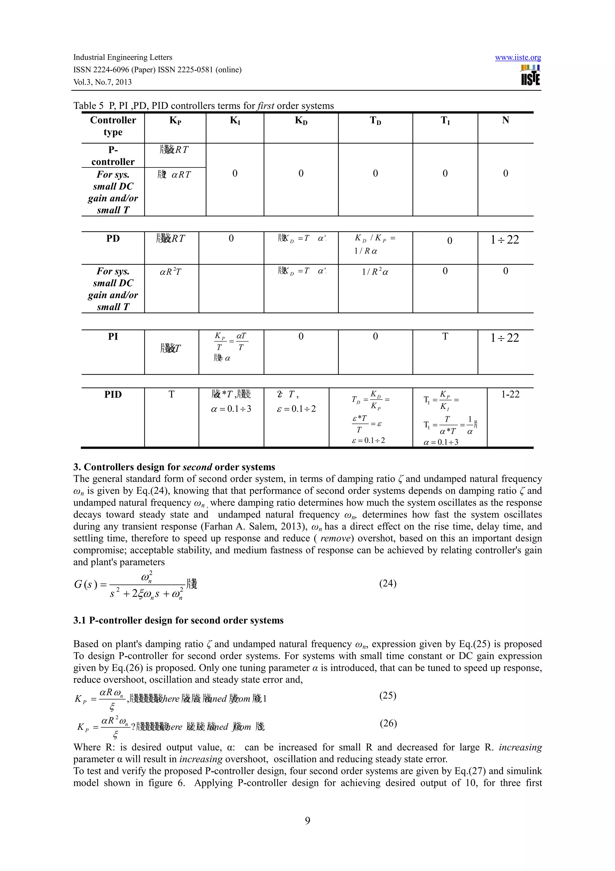
Table 10 P, PI , PD, PID controllers terms for
Controller
type
KP
P-controller nRα ω
ξ
For systems
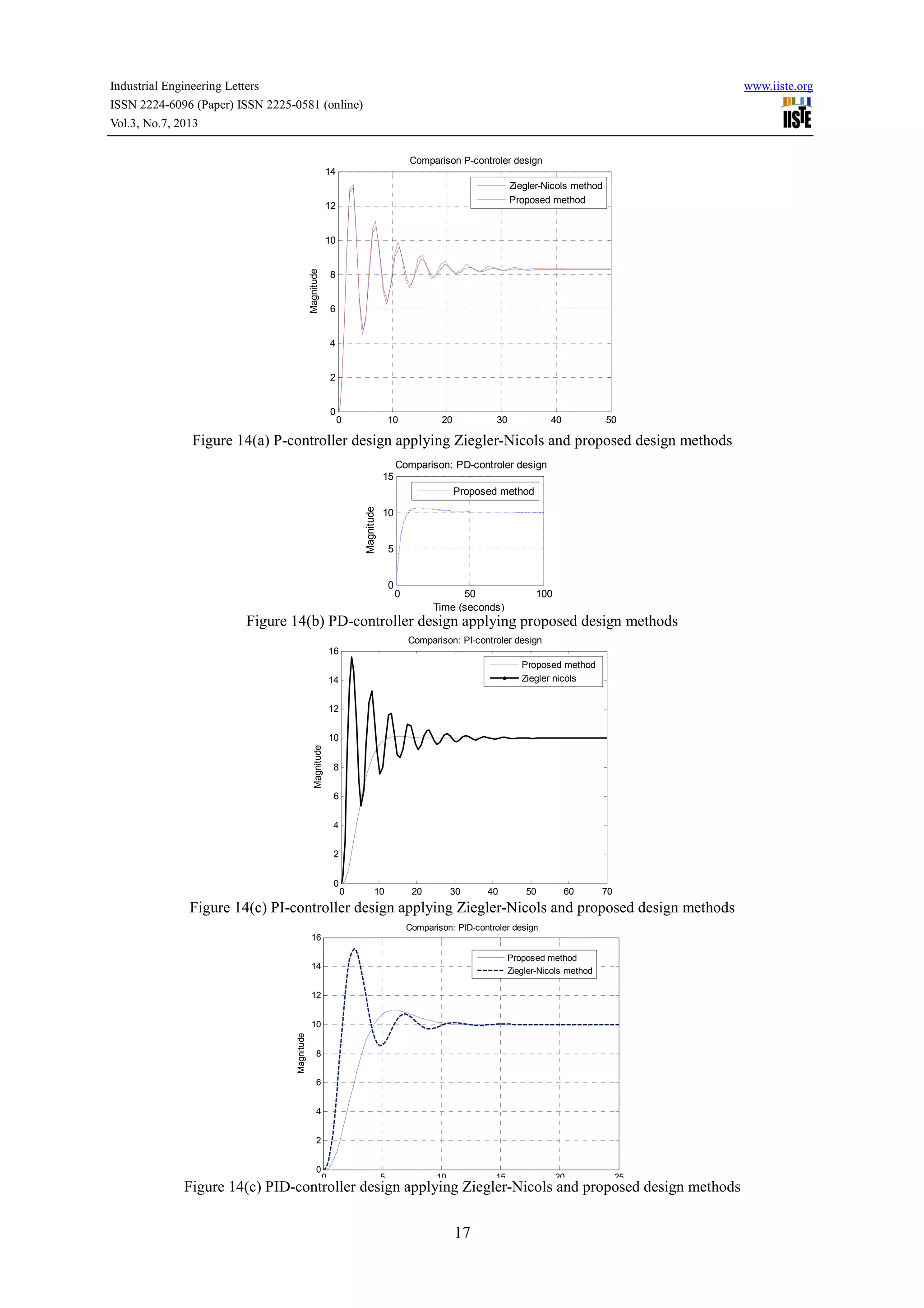
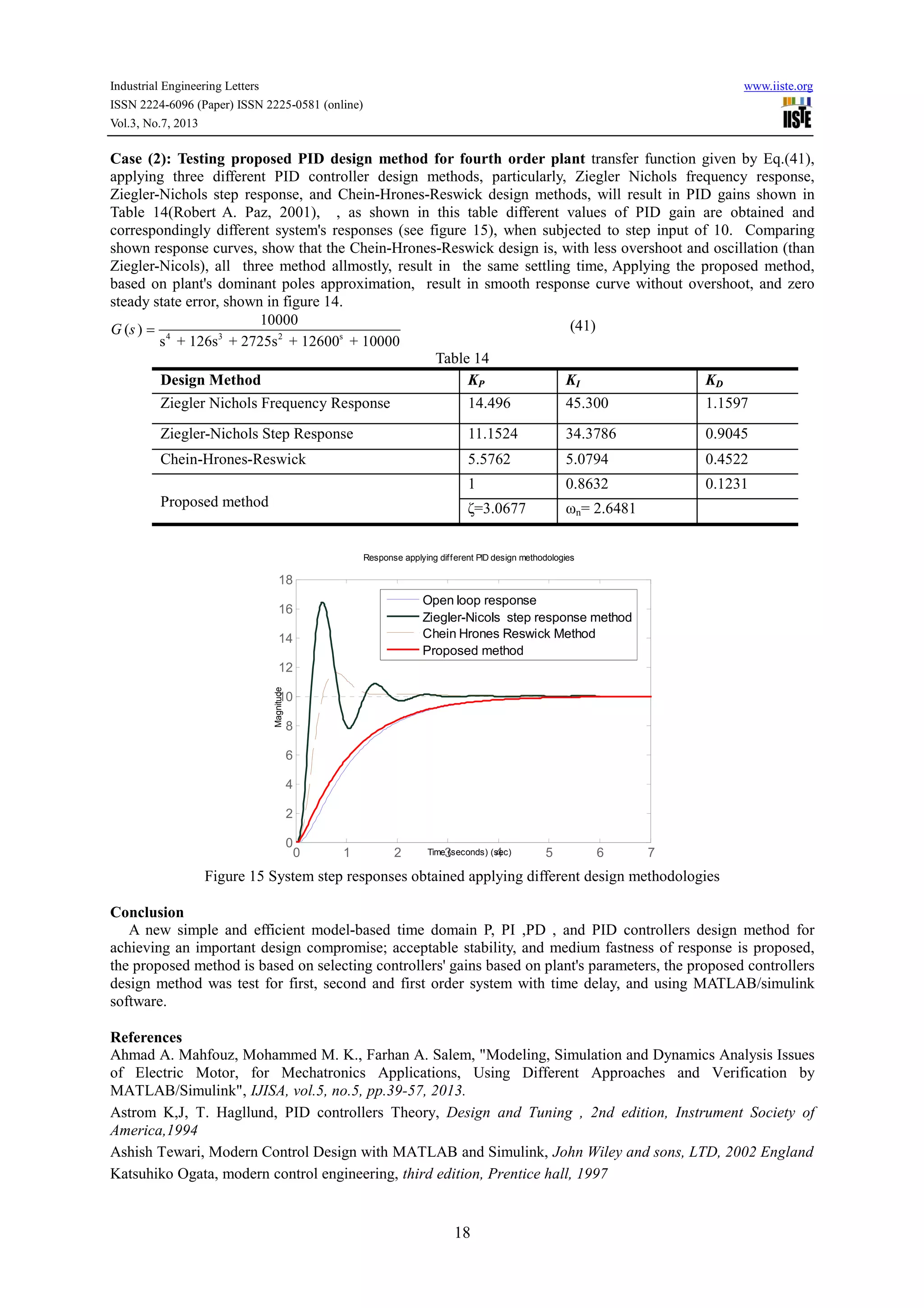
with small
DC gain
and/or small
T
2
nRα ω
ξ
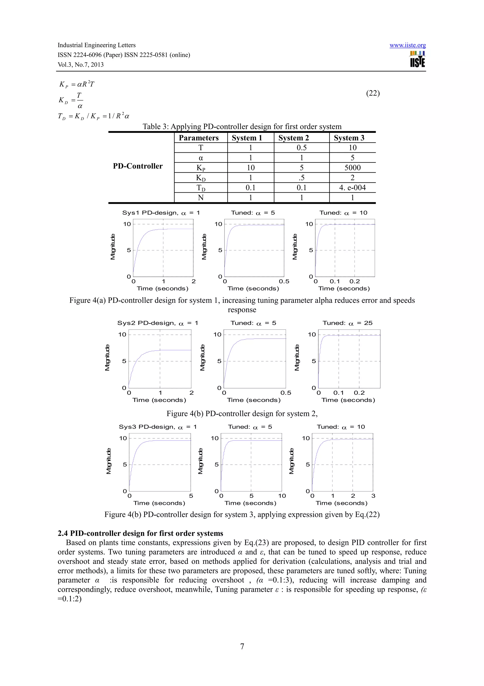
PD
n
Rα
ξω
Systems with
small DC
gain and/or
small T
2
n
Rα
ξω
PI
0.8 2
IKα
α = ÷
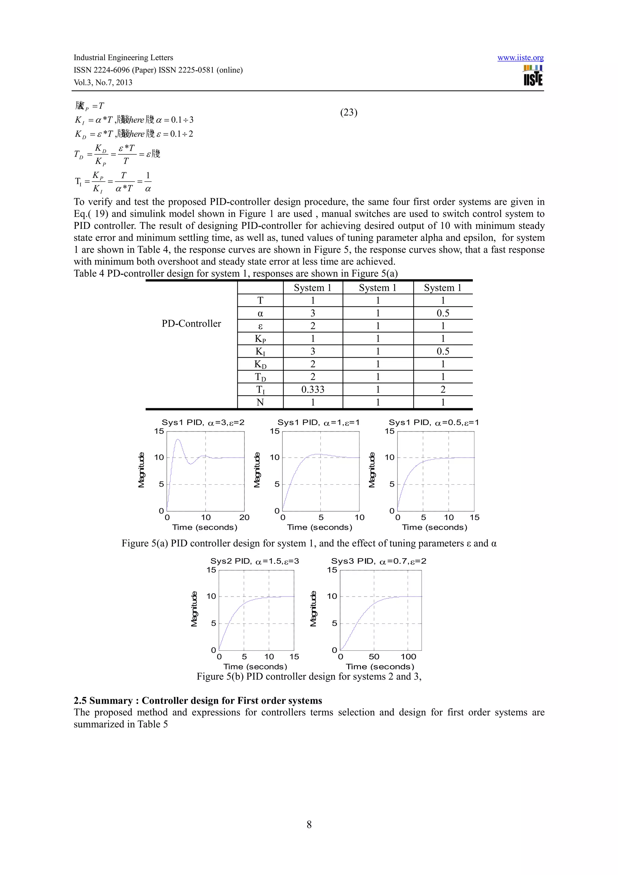
PID 1
,
2
nω
ε ε
ξ
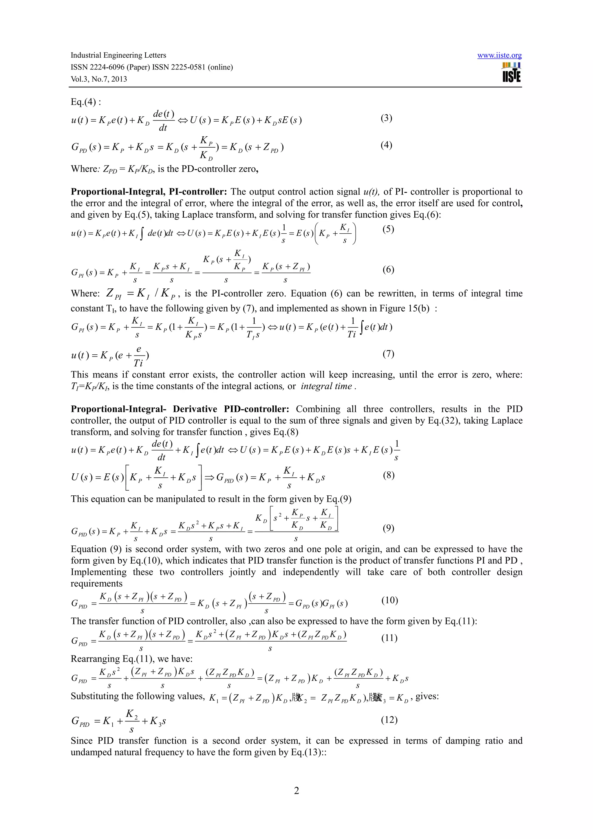
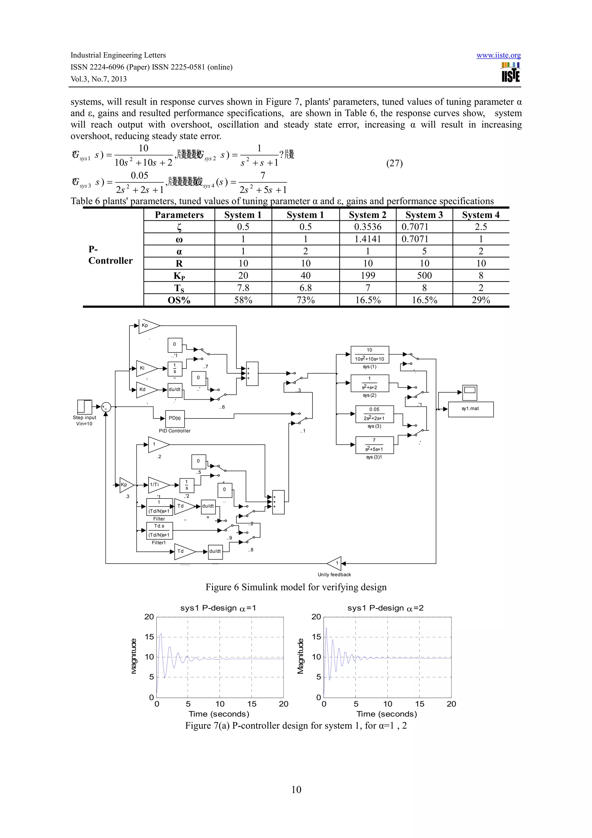
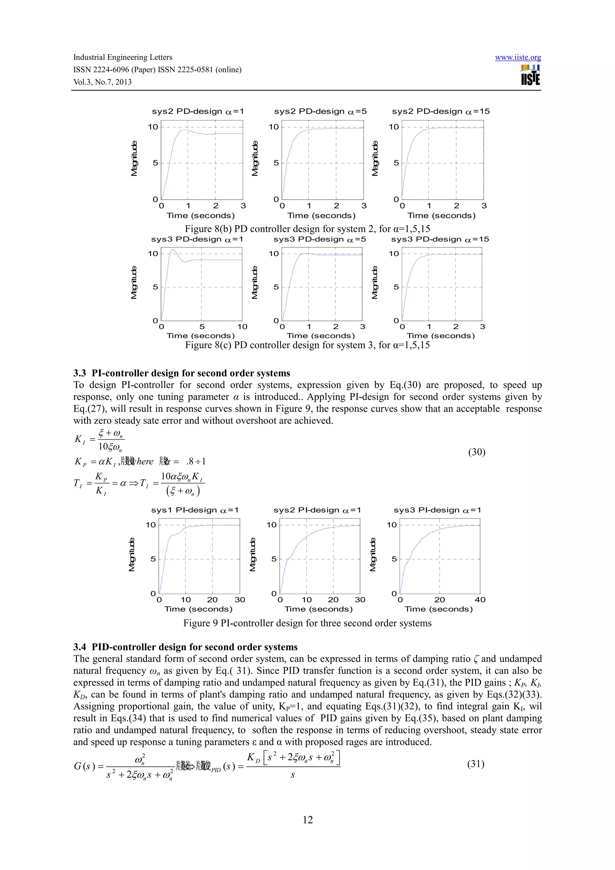
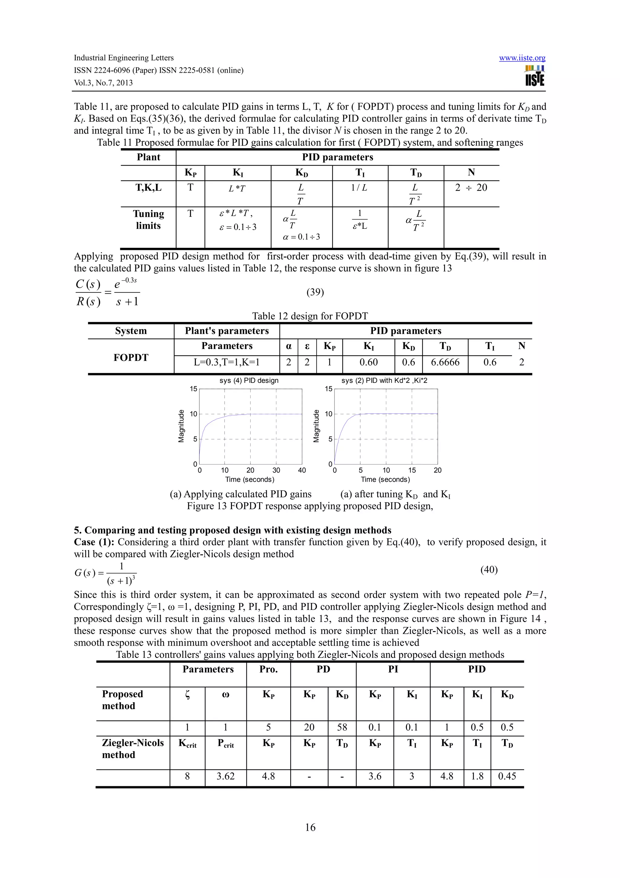
4. PID Controller for first order plus delay time
A large number of industrial plants can approximately be modeled by a first order plus time delay (FOPTD)
(Katsuhiko Ogata, 2010)(Saeed Tavakoli et al, 2003)
model with dead-time ,it transfer function is given by Eq.(38) and
s-shape curve with no overshoot is called
and time constant T, these two constants can be determined by drawing a tangent line at the infl
the s-shaped curve, and finding the intersection of the tangent line with time axis and steady state level
Figure 12), then the transfer function of these
transport lag and given by Eq.(38)[]:
( )
( ) 1
Ls
C s Ke
R s Ts
−
=
+
Figure 12 s-shaped curve with terminology (Farhan A. Salem, 2013)
Based on plant's delay time L, time constant T, and steady state level
0581 (online)
15
3.5 Summary: Controller design for second order systems
The proposed method for second order systems and expressions for controllers terms selection and design are
Table 10 P, PI , PD, PID controllers terms for second order systems
KI KD TD
0 0 0
0 2.9* nRα ξω 2 2
2.9 nξ ω
0 2
nRα ξω 2 2
nξ ω
10
n
n
ξ ω
ξω
+
0 0 I
I
T
T
,牋? .1 2
2
nω
ε ε
ξ
= ÷
1
?牋
2
? .58 1.5
n
α
ξω
α = ÷
2 n
α
ξω εω
4. PID Controller for first order plus delay time ( FOPDT) process
lants can approximately be modeled by a first order plus time delay (FOPTD)
(Katsuhiko Ogata, 2010)(Saeed Tavakoli et al, 2003). FOPDT models are a combination of a first
transfer function is given by Eq.(38) and it response curve is shown in Figure 12, this
is called reaction curve, it is characterized by two constants ; the delay time
, these two constants can be determined by drawing a tangent line at the infl
shaped curve, and finding the intersection of the tangent line with time axis and steady state level
Figure 12), then the transfer function of these-shaped curve can be approximated by first order system with
nd given by Eq.(38)[]:
shaped curve with terminology (Farhan A. Salem, 2013)
Based on plant's delay time L, time constant T, and steady state level K, ( see Eq. (12)). The formulae listed in
www.iiste.org
selection and design are
TI N
0 0
0 1-22
0 1-22
( )
10
P
I
I
n I
I
n
K
T
K
K
T
α
αξω
ξ ω
= = ⇒
=
+
1-22
2
n
ξ
εω
1-22
lants can approximately be modeled by a first order plus time delay (FOPTD)
. FOPDT models are a combination of a first-order process
esponse curve is shown in Figure 12, this
is characterized by two constants ; the delay time L,
, these two constants can be determined by drawing a tangent line at the inflection point of
shaped curve, and finding the intersection of the tangent line with time axis and steady state level K, (see
shaped curve can be approximated by first order system with
(38)
shaped curve with terminology (Farhan A. Salem, 2013)
, ( see Eq. (12)). The formulae listed in](https://image.slidesharecdn.com/newcontrollersefficientmodel-baseddesignmethod-130805072244-phpapp02/75/New-controllers-efficient-model-based-design-method-15-2048.jpg)


![Industrial Engineering Letters
ISSN 2224-6096 (Paper) ISSN 2225-0581 (online
Vol.3, No.7, 2013
3.5 Summary: Controller design for second order systems
The proposed method for second order systems and expressions for controllers terms
summarized in Table 10
Table 10 P, PI , PD, PID controllers terms for
Controller
type
KP
P-controller nRα ω
ξ
For systems
with small
DC gain
and/or small
T
2
nRα ω
ξ
PD
n
Rα
ξω
Systems with
small DC
gain and/or
small T
2
n
Rα
ξω
PI
0.8 2
IKα
α = ÷
PID 1
,
2
nω
ε ε
ξ
4. PID Controller for first order plus delay time
A large number of industrial plants can approximately be modeled by a first order plus time delay (FOPTD)
(Katsuhiko Ogata, 2010)(Saeed Tavakoli et al, 2003)
model with dead-time ,it transfer function is given by Eq.(38) and
s-shape curve with no overshoot is called
and time constant T, these two constants can be determined by drawing a tangent line at the infl
the s-shaped curve, and finding the intersection of the tangent line with time axis and steady state level
Figure 12), then the transfer function of these
transport lag and given by Eq.(38)[]:
( )
( ) 1
Ls
C s Ke
R s Ts
−
=
+
Figure 12 s-shaped curve with terminology (Farhan A. Salem, 2013)
Based on plant's delay time L, time constant T, and steady state level
0581 (online)
15
3.5 Summary: Controller design for second order systems
The proposed method for second order systems and expressions for controllers terms selection and design are
Table 10 P, PI , PD, PID controllers terms for second order systems
KI KD TD
0 0 0
0 2.9* nRα ξω 2 2
2.9 nξ ω
0 2
nRα ξω 2 2
nξ ω
10
n
n
ξ ω
ξω
+
0 0 I
I
T
T
,牋? .1 2
2
nω
ε ε
ξ
= ÷
1
?牋
2
? .58 1.5
n
α
ξω
α = ÷
2 n
α
ξω εω
4. PID Controller for first order plus delay time ( FOPDT) process
lants can approximately be modeled by a first order plus time delay (FOPTD)
(Katsuhiko Ogata, 2010)(Saeed Tavakoli et al, 2003). FOPDT models are a combination of a first
transfer function is given by Eq.(38) and it response curve is shown in Figure 12, this
is called reaction curve, it is characterized by two constants ; the delay time
, these two constants can be determined by drawing a tangent line at the infl
shaped curve, and finding the intersection of the tangent line with time axis and steady state level
Figure 12), then the transfer function of these-shaped curve can be approximated by first order system with
nd given by Eq.(38)[]:
shaped curve with terminology (Farhan A. Salem, 2013)
Based on plant's delay time L, time constant T, and steady state level K, ( see Eq. (12)). The formulae listed in
www.iiste.org
selection and design are
TI N
0 0
0 1-22
0 1-22
( )
10
P
I
I
n I
I
n
K
T
K
K
T
α
αξω
ξ ω
= = ⇒
=
+
1-22
2
n
ξ
εω
1-22
lants can approximately be modeled by a first order plus time delay (FOPTD)
. FOPDT models are a combination of a first-order process
esponse curve is shown in Figure 12, this
is characterized by two constants ; the delay time L,
, these two constants can be determined by drawing a tangent line at the inflection point of
shaped curve, and finding the intersection of the tangent line with time axis and steady state level K, (see
shaped curve can be approximated by first order system with
(38)
shaped curve with terminology (Farhan A. Salem, 2013)
, ( see Eq. (12)). The formulae listed in](https://crownmelresort.com/image.slidesharecdn.com/newcontrollersefficientmodel-baseddesignmethod-130805072244-phpapp02/75/New-controllers-efficient-model-based-design-method-15-2048.jpg)


This document proposes new methods for designing P, PI, PD, and PID controllers based on selecting the controller gains based on the plant's parameters. The goal is to achieve acceptable stability and medium fast response. Expressions are proposed for calculating the controller gains for first-order, second-order, and time-delay systems based on the plant's time constant, damping ratio, and natural frequency. The proposed controller design methods are tested on first, second, and first-order systems with time delay using MATLAB/Simulink. The results show the methods can achieve acceptable stability and medium fast response with minimum steady state error by selecting a single tuning parameter.