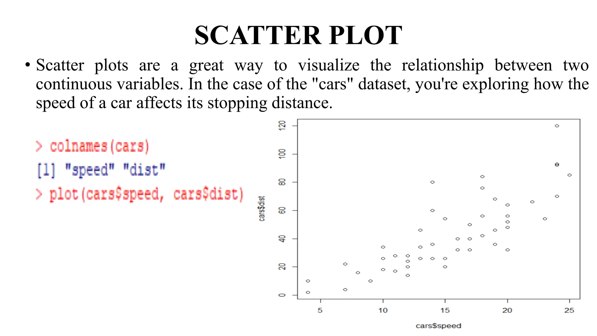
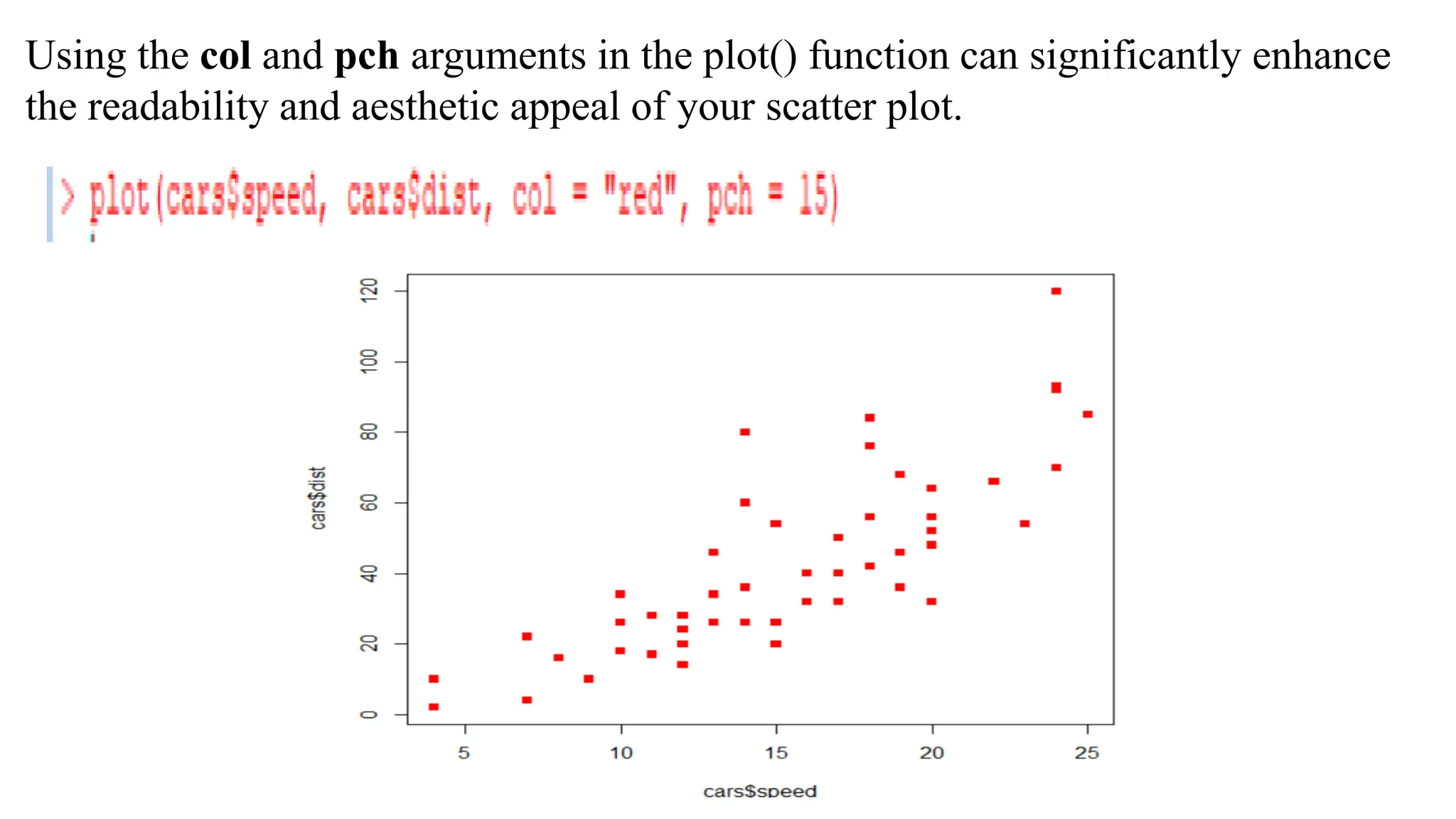
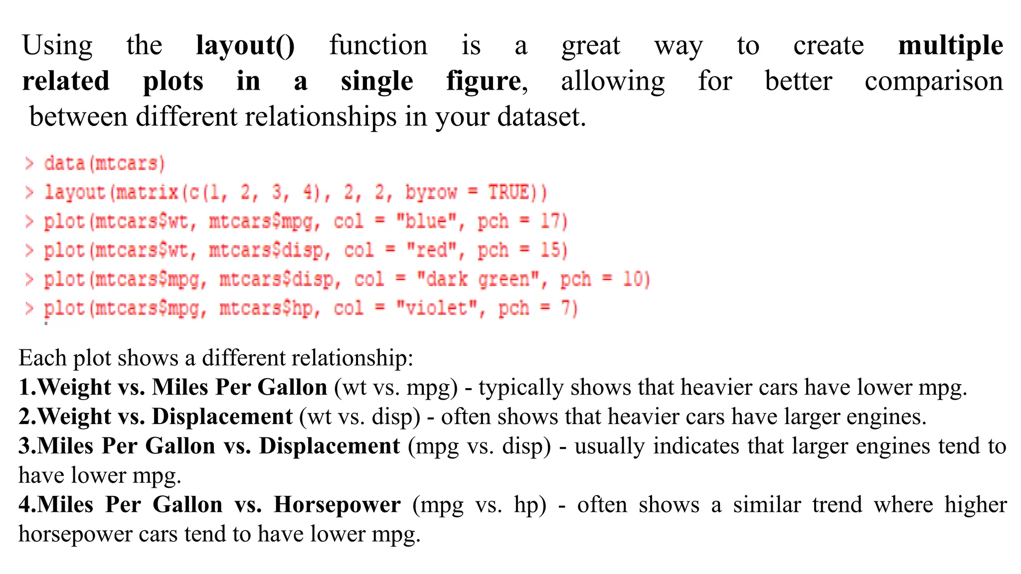
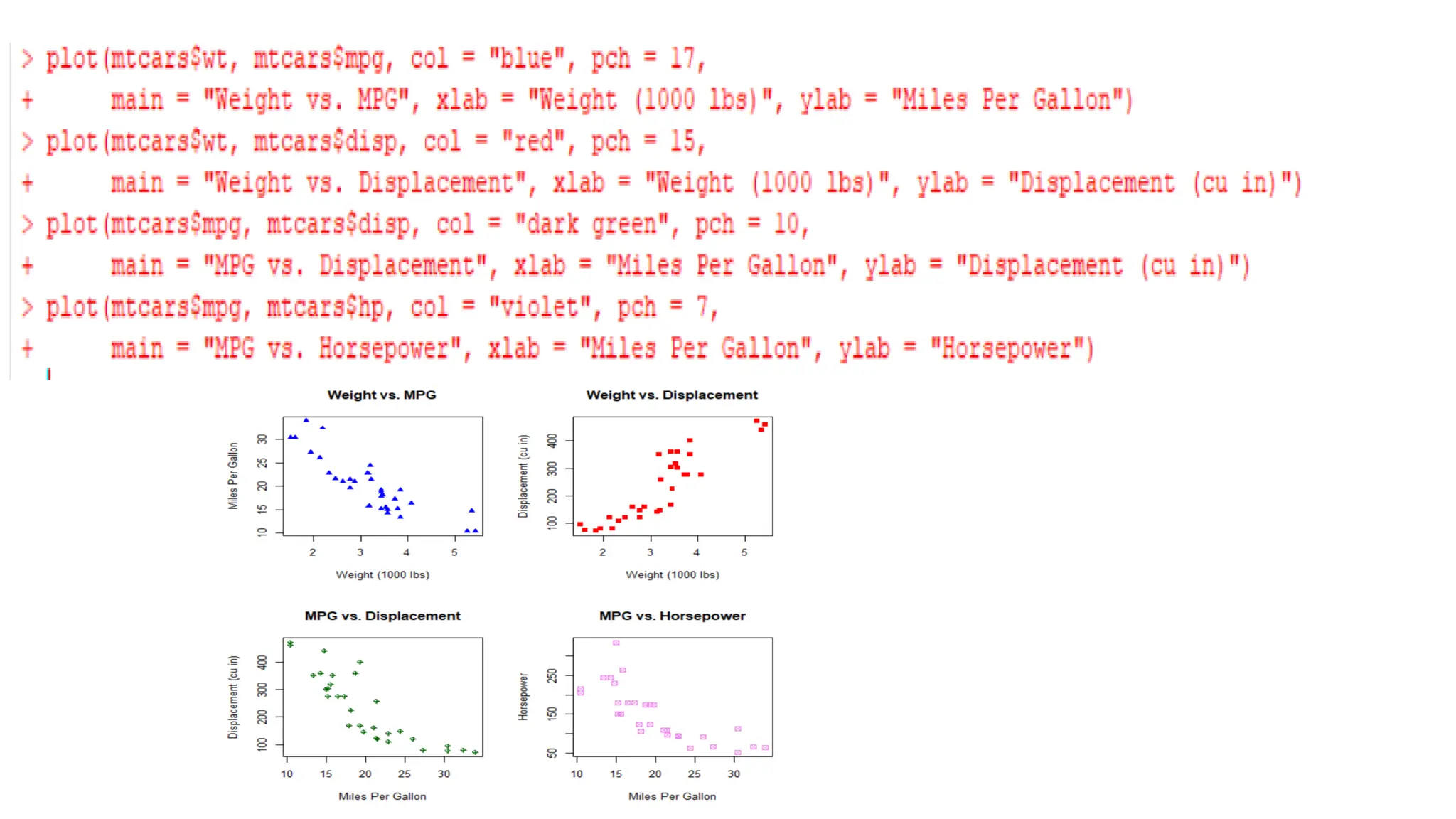
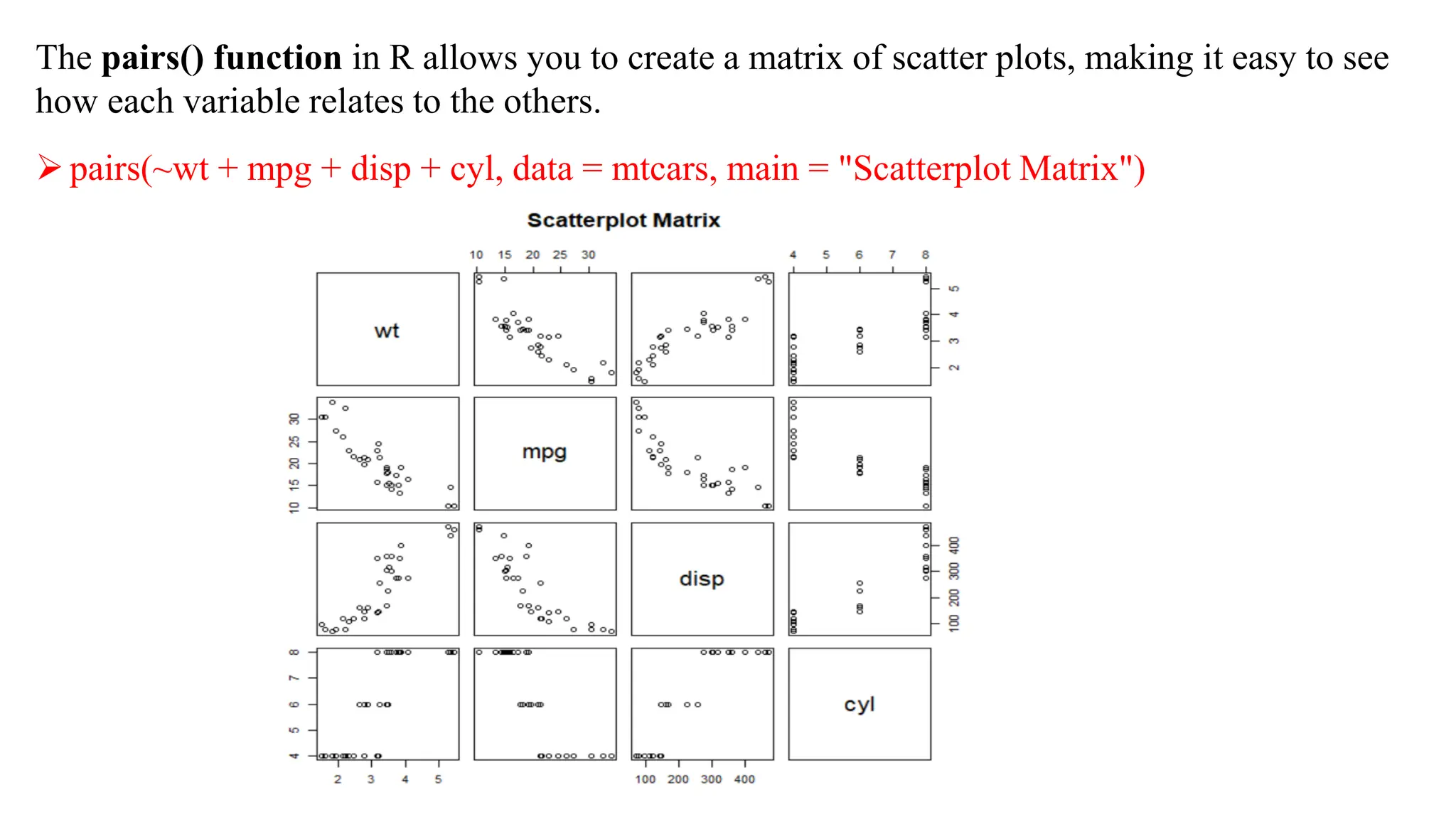
Data Analytics With R
Prof.Navyashree K S
Assistant Professor
Dept.of CSE (Data Science)
Sub code: BDS306C
Module 4
GRAPHICS USING R
Exploratory Data Analysis :Exploratory Data Analysis (EDA) is a visual
based method used to analyze datasets and to summarize their main
characteristics.
•Maximize Insight into a Data Set: Use summary statistics (mean, median,
mode, standard deviation) and visualizations(histograms, box plots) to get an
overall sense of the data distribution.
•Uncover Underlying Structure: Apply techniques like clustering (e.g., k-
means, hierarchical clustering) and dimensionality reduction (e.g., PCA) to
identify patterns and groupings.
•Extract Important Variables: Use correlation matrices, feature importance
from models, or techniques like recursive feature elimination to identify which
variables contribute most to your target outcome.
•Detect Outliers and Anomalies: Visual methods (box plots, scatter plots)
and statistical tests (Z-scores, IQR) can help identify unusual observations
that might affect model performance.
•Test Underlying Assumptions: Check assumptions of statistical tests and
models using Q-Q plots, residual plots, and other diagnostic tools.
•Develop Parsimonious Models: Focus on simpler models that adequately
capture the data patterns, using techniques like regularization to avoid
overfitting.
•Determine Optimal Factor Settings: Use techniques like factorial design
or response surface methodology to explore the effects of different factors
on outcomes and optimize settings.
MAIN GRAPHICAL PACKAGES
Base Graphics:
•The simplest way to create plots in R.
•Good for quick and straightforward visualizations.
•Limited customization options and flexibility.
Example: plot(), hist(), boxplot().
Grid Graphics:
•Built on a more sophisticated framework compared to base graphics.
•Allows for more control over layout and placement of graphical elements.
•Does not natively support certain types of plots like scatter plots without
additional functions.
Example: grid.newpage(), grid.rect().
Lattice Graphics:
•Designed for creating trellis graphs, which are particularly useful for multivariate
data.
•Supports conditioning, allowing you to create multiple panels based on factor
levels.
•More structured than base graphics and provides better handling of complex layouts.
Example: xyplot(), bwplot(), histogram().
ggplot2:
•Based on the "Grammar of Graphics," which provides a coherent way to describe
and build visualizations.
•Highly customizable and capable of creating complex multi-layered graphics.
•Supports various data types and allows for easy addition of aesthetic mappings (like
color, size, shape).
Example: ggplot(data, aes(x, y)) + geom_point(), geom_smooth(), facet_wrap().
PIE CHART
Creating a pie chart in R is straightforward using the pie() function.
Syntax: pie(x, labels, radius, main, col, clockwise)
Parameters
•x: A numeric vector representing the values for each slice of the pie.
•labels: A vector of descriptions for each slice.
•radius: Controls the radius of the pie chart; values typically range from -1 to +1.
•main: The title of the pie chart.
•col: A color palette for the slices. You can use predefined palettes like rainbow()
or heat.colors().
•clockwise: A logical value (TRUE for clockwise, FALSE for anti-clockwise) to
control the direction of the slices.
To create a 3D pie chart in R, you can use the plotrix package, which provides the
pie3D() function. This function allows you to create a visually appealing 3D
representation of your data.
install.packages("plotrix") # Install the package
library(plotrix) # Load the package
• Scatter plots are a great way to visualize the relationship between two
continuous variables. In the case of the "cars" dataset, you're exploring how the
speed of a car affects its stopping distance.
SCATTER PLOT
Using the col and pch arguments in the plot() function can significantly enhance
the readability and aesthetic appeal of your scatter plot.
Using the layout() function is a great way to create multiple
related plots in a single figure, allowing for better comparison
between different relationships in your dataset.
Each plot shows a different relationship:
1.Weight vs. Miles Per Gallon (wt vs. mpg) - typically shows that heavier cars have lower mpg.
2.Weight vs. Displacement (wt vs. disp) - often shows that heavier cars have larger engines.
3.Miles Per Gallon vs. Displacement (mpg vs. disp) - usually indicates that larger engines tend to
have lower mpg.
4.Miles Per Gallon vs. Horsepower (mpg vs. hp) - often shows a similar trend where higher
horsepower cars tend to have lower mpg.
The pairs() function in R allows you to create a matrix of scatter plots, making it easy to see
how each variable relates to the others.
➢pairs(~wt + mpg + disp + cyl, data = mtcars, main = "Scatterplot Matrix")
The xyplot() function from the lattice package is a powerful alternative to base R
plotting functions, allowing for enhanced visualization of relationships between variable
The ggplot2 package is an incredibly powerful tool for creating visualizations in R, using
a layered approach that allows for extensive customization. The way you described using
ggplot() with aes() and geom_point() is a perfect introduction to this system.
The facet_wrap() function in ggplot2 allows you to create multiple panels (facets) of
plots based on the values of a categorical variable.
This is similar to how lattice handles faceting. Additionally, the theme() function lets
you customize the appearance of the plot, including the orientation of axis text.

M4_DAR_part1. module part 4 analystics with r

  • 1.
    Data Analytics WithR Prof.Navyashree K S Assistant Professor Dept.of CSE (Data Science) Sub code: BDS306C Module 4
  • 2.
    GRAPHICS USING R ExploratoryData Analysis :Exploratory Data Analysis (EDA) is a visual based method used to analyze datasets and to summarize their main characteristics. •Maximize Insight into a Data Set: Use summary statistics (mean, median, mode, standard deviation) and visualizations(histograms, box plots) to get an overall sense of the data distribution. •Uncover Underlying Structure: Apply techniques like clustering (e.g., k- means, hierarchical clustering) and dimensionality reduction (e.g., PCA) to identify patterns and groupings. •Extract Important Variables: Use correlation matrices, feature importance from models, or techniques like recursive feature elimination to identify which variables contribute most to your target outcome.
  • 3.
    •Detect Outliers andAnomalies: Visual methods (box plots, scatter plots) and statistical tests (Z-scores, IQR) can help identify unusual observations that might affect model performance. •Test Underlying Assumptions: Check assumptions of statistical tests and models using Q-Q plots, residual plots, and other diagnostic tools. •Develop Parsimonious Models: Focus on simpler models that adequately capture the data patterns, using techniques like regularization to avoid overfitting. •Determine Optimal Factor Settings: Use techniques like factorial design or response surface methodology to explore the effects of different factors on outcomes and optimize settings.
  • 4.
    MAIN GRAPHICAL PACKAGES BaseGraphics: •The simplest way to create plots in R. •Good for quick and straightforward visualizations. •Limited customization options and flexibility. Example: plot(), hist(), boxplot(). Grid Graphics: •Built on a more sophisticated framework compared to base graphics. •Allows for more control over layout and placement of graphical elements. •Does not natively support certain types of plots like scatter plots without additional functions. Example: grid.newpage(), grid.rect().
  • 5.
    Lattice Graphics: •Designed forcreating trellis graphs, which are particularly useful for multivariate data. •Supports conditioning, allowing you to create multiple panels based on factor levels. •More structured than base graphics and provides better handling of complex layouts. Example: xyplot(), bwplot(), histogram(). ggplot2: •Based on the "Grammar of Graphics," which provides a coherent way to describe and build visualizations. •Highly customizable and capable of creating complex multi-layered graphics. •Supports various data types and allows for easy addition of aesthetic mappings (like color, size, shape). Example: ggplot(data, aes(x, y)) + geom_point(), geom_smooth(), facet_wrap().
  • 6.
    PIE CHART Creating apie chart in R is straightforward using the pie() function. Syntax: pie(x, labels, radius, main, col, clockwise) Parameters •x: A numeric vector representing the values for each slice of the pie. •labels: A vector of descriptions for each slice. •radius: Controls the radius of the pie chart; values typically range from -1 to +1. •main: The title of the pie chart. •col: A color palette for the slices. You can use predefined palettes like rainbow() or heat.colors(). •clockwise: A logical value (TRUE for clockwise, FALSE for anti-clockwise) to control the direction of the slices.
  • 8.
    To create a3D pie chart in R, you can use the plotrix package, which provides the pie3D() function. This function allows you to create a visually appealing 3D representation of your data. install.packages("plotrix") # Install the package library(plotrix) # Load the package
  • 9.
    • Scatter plotsare a great way to visualize the relationship between two continuous variables. In the case of the "cars" dataset, you're exploring how the speed of a car affects its stopping distance. SCATTER PLOT
  • 10.
    Using the coland pch arguments in the plot() function can significantly enhance the readability and aesthetic appeal of your scatter plot.
  • 11.
    Using the layout()function is a great way to create multiple related plots in a single figure, allowing for better comparison between different relationships in your dataset. Each plot shows a different relationship: 1.Weight vs. Miles Per Gallon (wt vs. mpg) - typically shows that heavier cars have lower mpg. 2.Weight vs. Displacement (wt vs. disp) - often shows that heavier cars have larger engines. 3.Miles Per Gallon vs. Displacement (mpg vs. disp) - usually indicates that larger engines tend to have lower mpg. 4.Miles Per Gallon vs. Horsepower (mpg vs. hp) - often shows a similar trend where higher horsepower cars tend to have lower mpg.
  • 13.
    The pairs() functionin R allows you to create a matrix of scatter plots, making it easy to see how each variable relates to the others. ➢pairs(~wt + mpg + disp + cyl, data = mtcars, main = "Scatterplot Matrix")
  • 14.
    The xyplot() functionfrom the lattice package is a powerful alternative to base R plotting functions, allowing for enhanced visualization of relationships between variable
  • 15.
    The ggplot2 packageis an incredibly powerful tool for creating visualizations in R, using a layered approach that allows for extensive customization. The way you described using ggplot() with aes() and geom_point() is a perfect introduction to this system.
  • 16.
    The facet_wrap() functionin ggplot2 allows you to create multiple panels (facets) of plots based on the values of a categorical variable. This is similar to how lattice handles faceting. Additionally, the theme() function lets you customize the appearance of the plot, including the orientation of axis text.