Download as PDF, PPTX


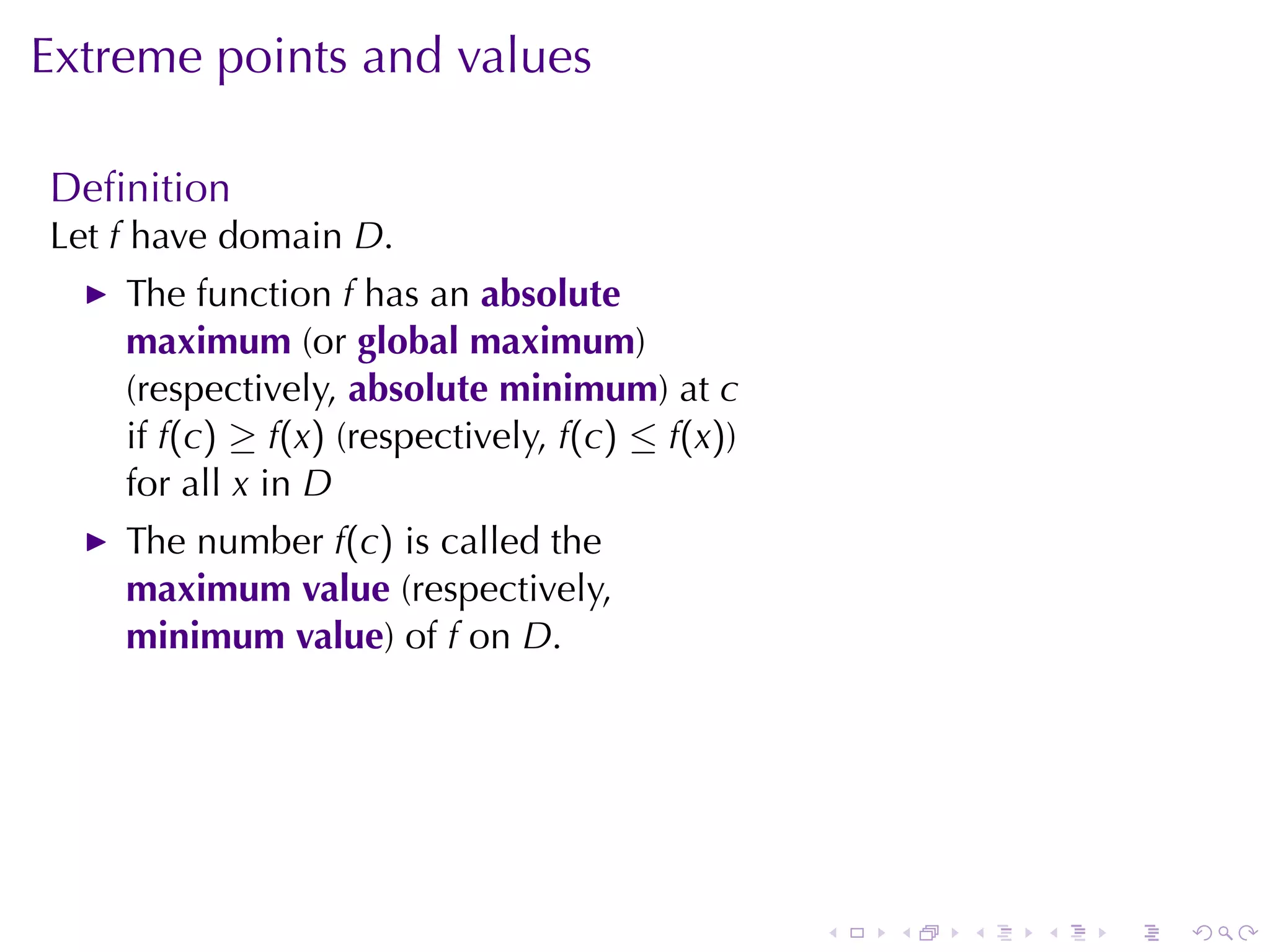
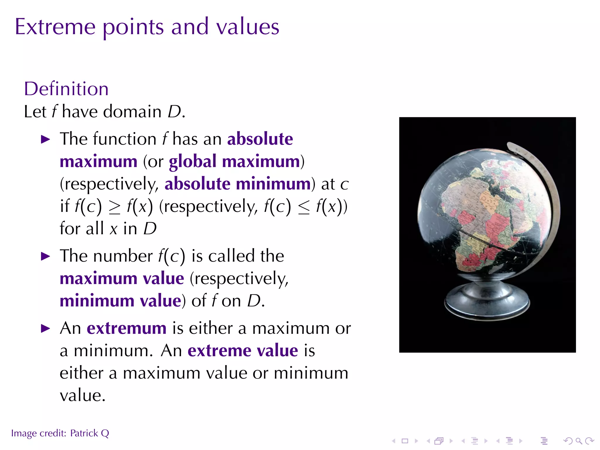
![Theorem (The Extreme Value Theorem)
Let f be a function which is continuous on the closed interval
[a, b]. Then f attains an absolute maximum value f(c) and an
absolute minimum value f(d) at numbers c and d in [a, b].
. . . . . .](https://image.slidesharecdn.com/lesson19-maximumandminimumvalues034slides-091105142101-phpapp01/75/Lesson19-Maximum-And-Minimum-Values-034-Slides-13-2048.jpg)
![Theorem (The Extreme Value Theorem)
Let f be a function which is continuous on the closed interval
[a, b]. Then f attains an absolute maximum value f(c) and an
absolute minimum value f(d) at numbers c and d in [a, b].
.
.
. .
a
. b
.
. . . . . .](https://image.slidesharecdn.com/lesson19-maximumandminimumvalues034slides-091105142101-phpapp01/75/Lesson19-Maximum-And-Minimum-Values-034-Slides-14-2048.jpg)
![Theorem (The Extreme Value Theorem)
Let f be a function which is continuous on the closed interval
[a, b]. Then f attains an absolute maximum value f(c) and an
absolute minimum value f(d) at numbers c and d in [a, b].
.
maximum .(c)
f
.
value
. .
minimum .(d)
f
.
value
. . ..
a
. d c
b
.
minimum maximum
. . . . . .](https://image.slidesharecdn.com/lesson19-maximumandminimumvalues034slides-091105142101-phpapp01/75/Lesson19-Maximum-And-Minimum-Values-034-Slides-15-2048.jpg)
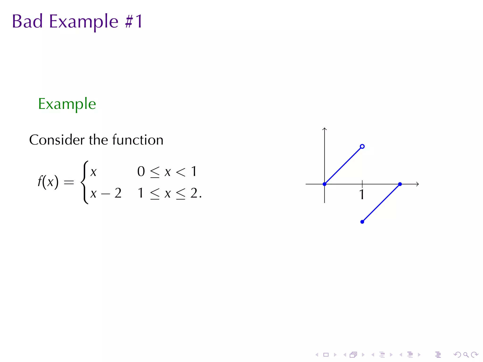
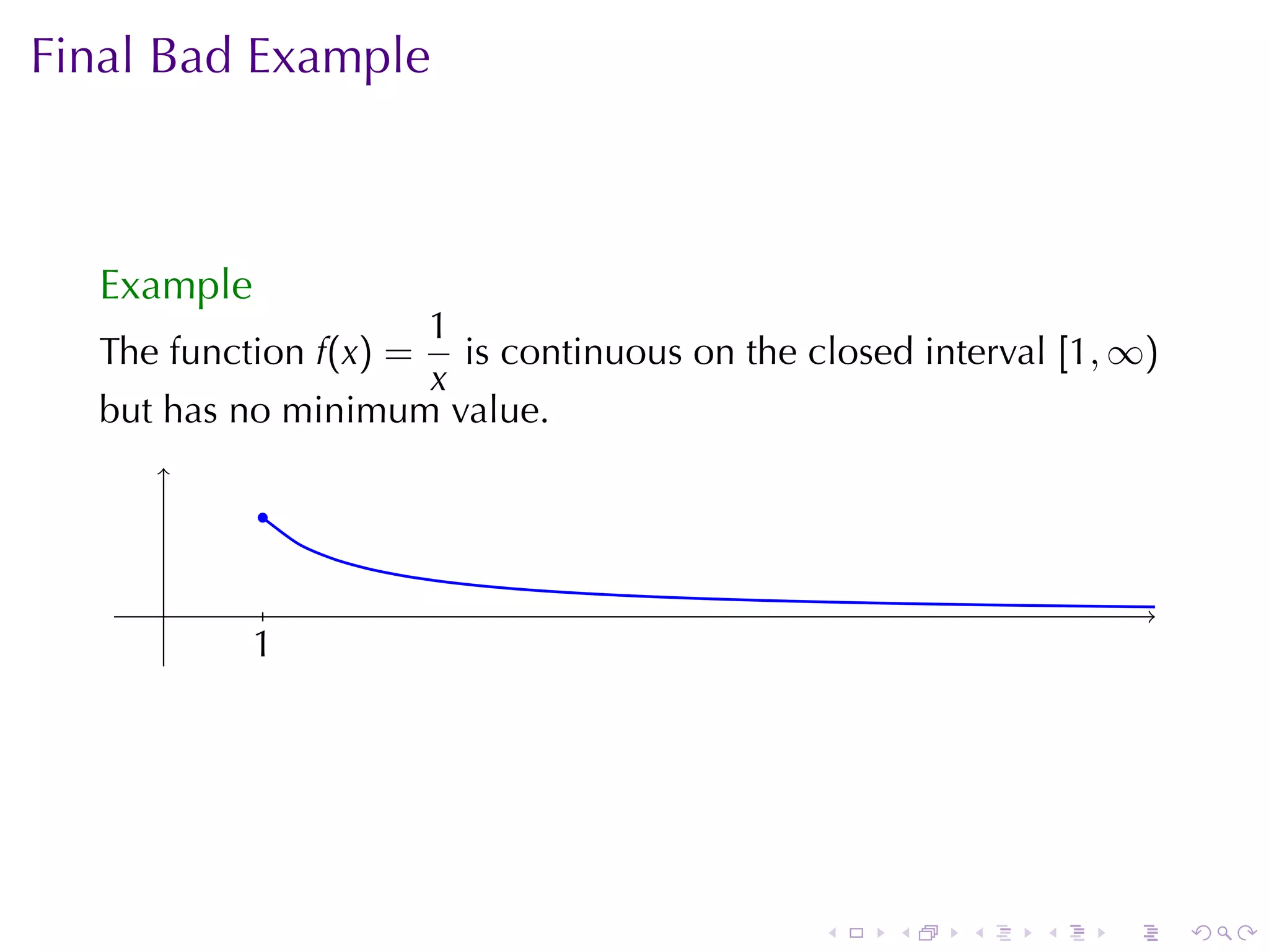
![Bad Example #1
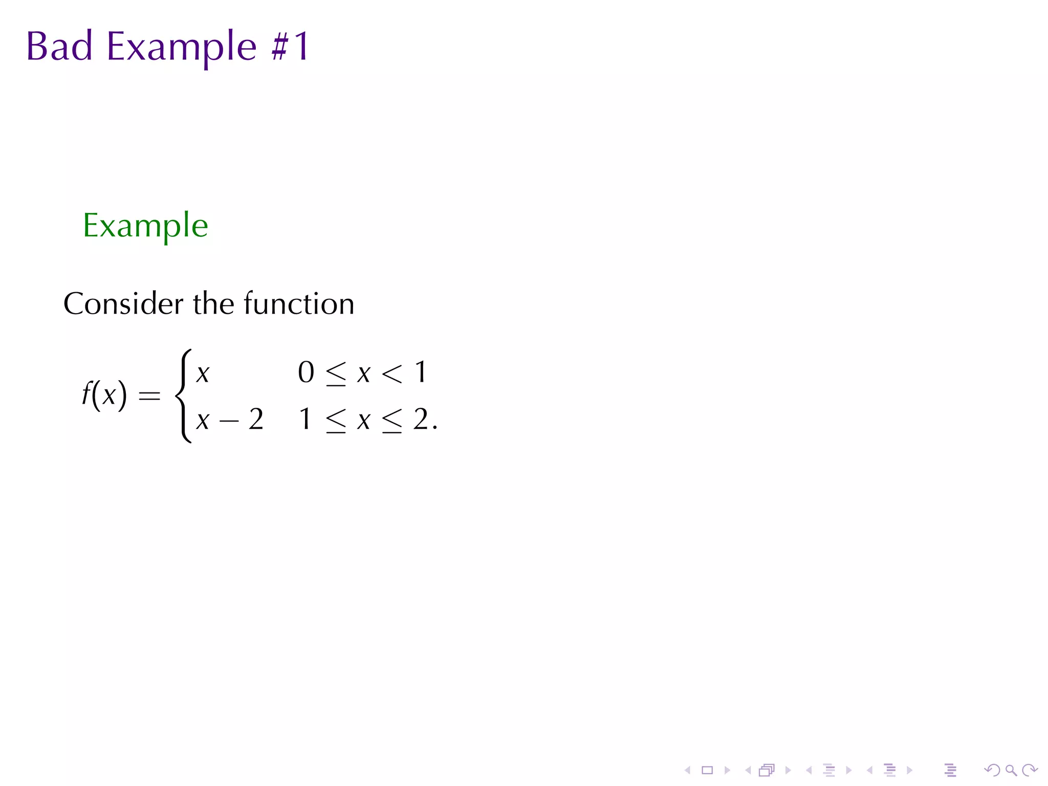
Example
Consider the function .
{
x 0≤x<1
f (x ) = . .
| .
x − 2 1 ≤ x ≤ 2. 1
.
.
Then although values of f(x) get arbitrarily close to 1 and never
bigger than 1, 1 is not the maximum value of f on [0, 1] because
it is never achieved.
. . . . . .](https://image.slidesharecdn.com/lesson19-maximumandminimumvalues034slides-091105142101-phpapp01/75/Lesson19-Maximum-And-Minimum-Values-034-Slides-19-2048.jpg)

![Flowchart for placing extrema
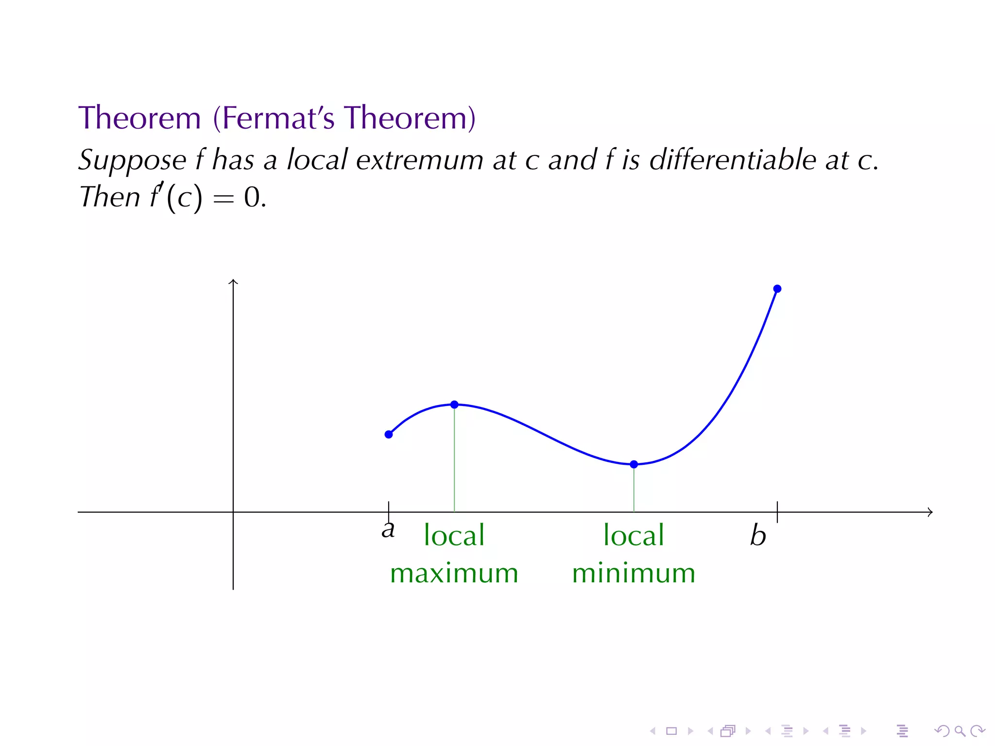
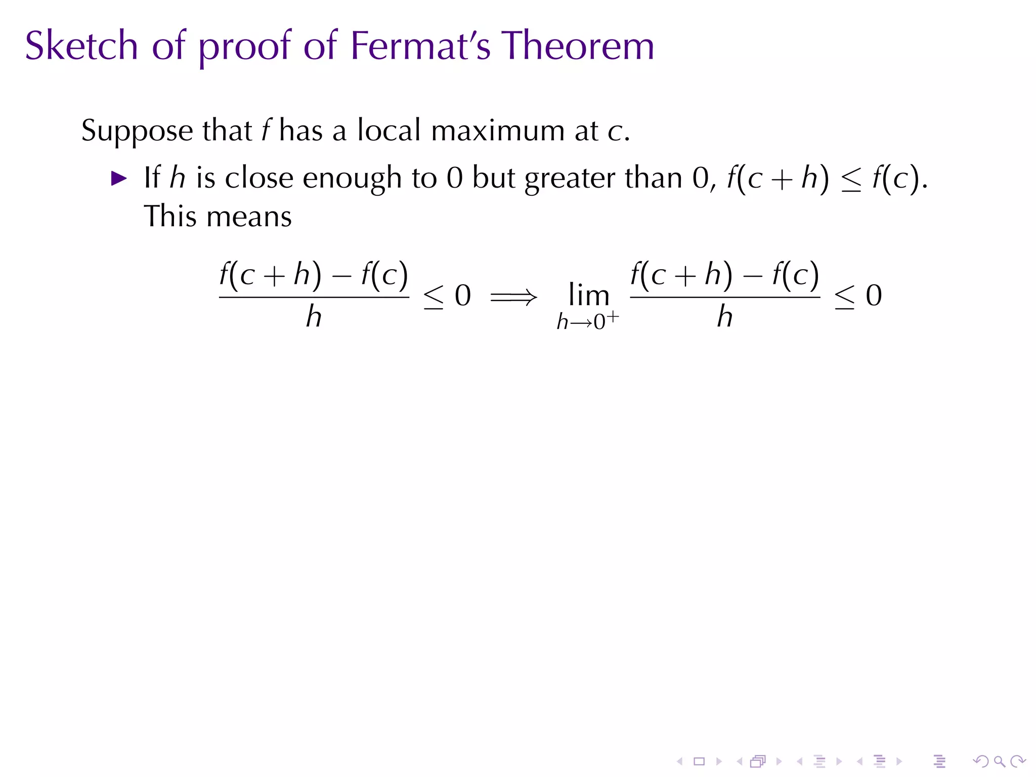
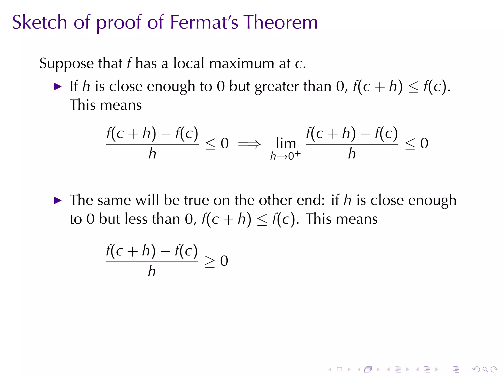
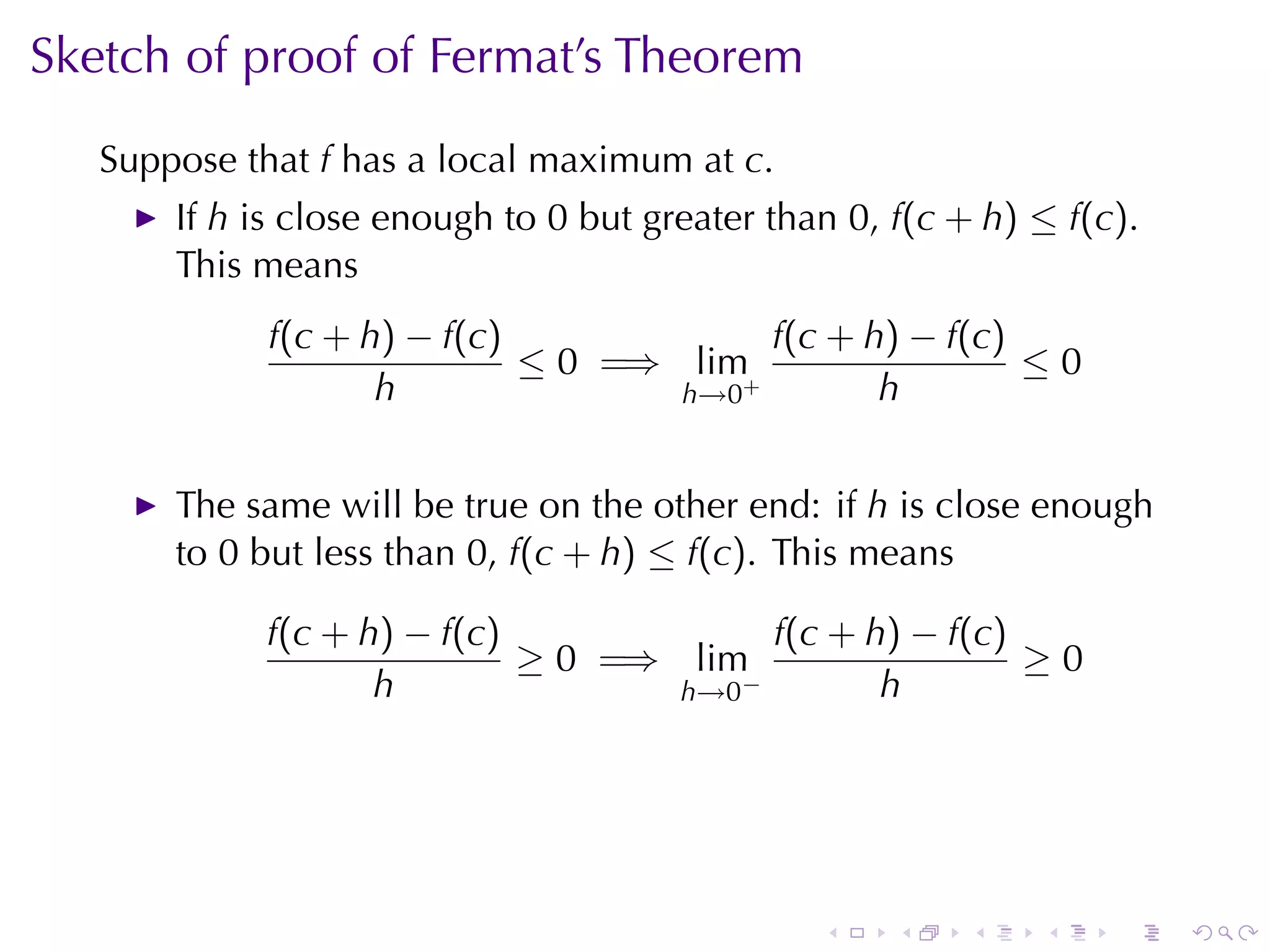
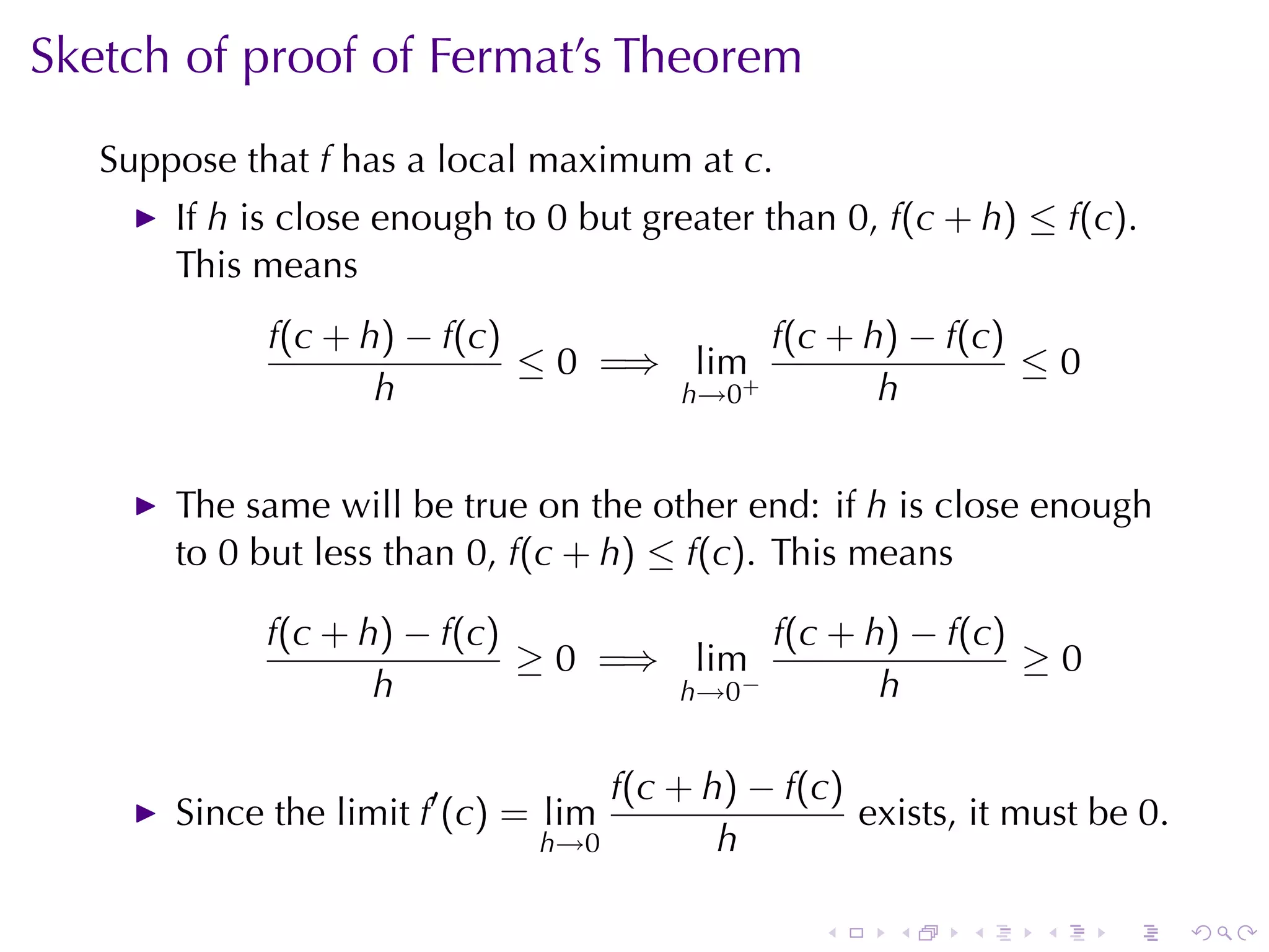
Thanks to Fermat
Suppose f is a continuous function on the closed, bounded
interval [a, b], and c is a global maximum point.
.
. . c is a
start
local max
. . .
Is c an Is f diff’ble f is not
n
.o n
.o
endpoint? at c? diff at c
y
. es y
. es
. c = a or .
f′ (c) = 0
c = b
. . . . . .](https://image.slidesharecdn.com/lesson19-maximumandminimumvalues034slides-091105142101-phpapp01/75/Lesson19-Maximum-And-Minimum-Values-034-Slides-41-2048.jpg)
![The Closed Interval Method
This means to find the maximum value of f on [a, b], we need to:
Evaluate f at the endpoints a and b
Evaluate f at the critical points or critical numbers x where
either f′ (x) = 0 or f is not differentiable at x.
The points with the largest function value are the global
maximum points
The points with the smallest or most negative function value
are the global minimum points.
. . . . . .](https://image.slidesharecdn.com/lesson19-maximumandminimumvalues034slides-091105142101-phpapp01/75/Lesson19-Maximum-And-Minimum-Values-034-Slides-42-2048.jpg)
![Example
Find the extreme values of f(x) = 2x − 5 on [−1, 2].
. . . . . .](https://image.slidesharecdn.com/lesson19-maximumandminimumvalues034slides-091105142101-phpapp01/75/Lesson19-Maximum-And-Minimum-Values-034-Slides-44-2048.jpg)
![Example
Find the extreme values of f(x) = 2x − 5 on [−1, 2].
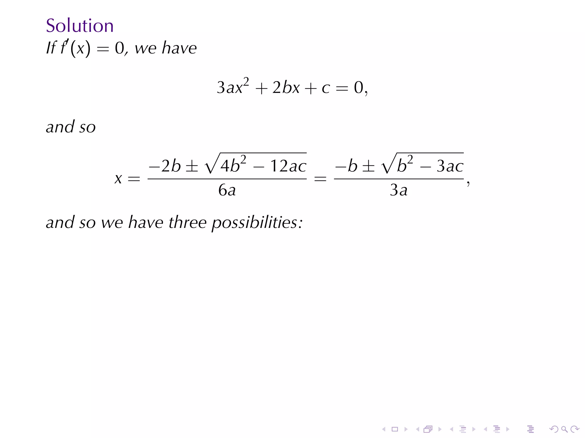
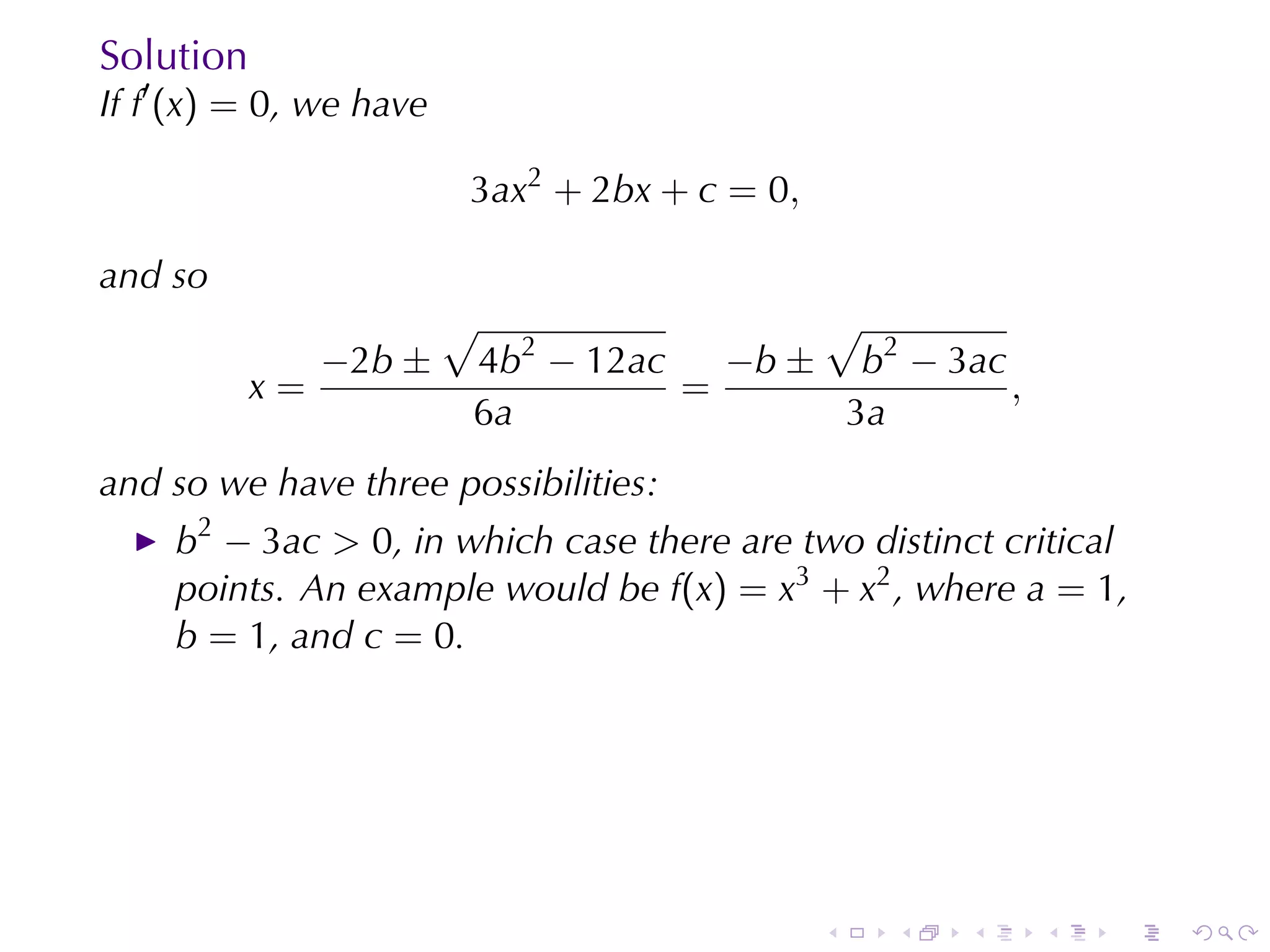
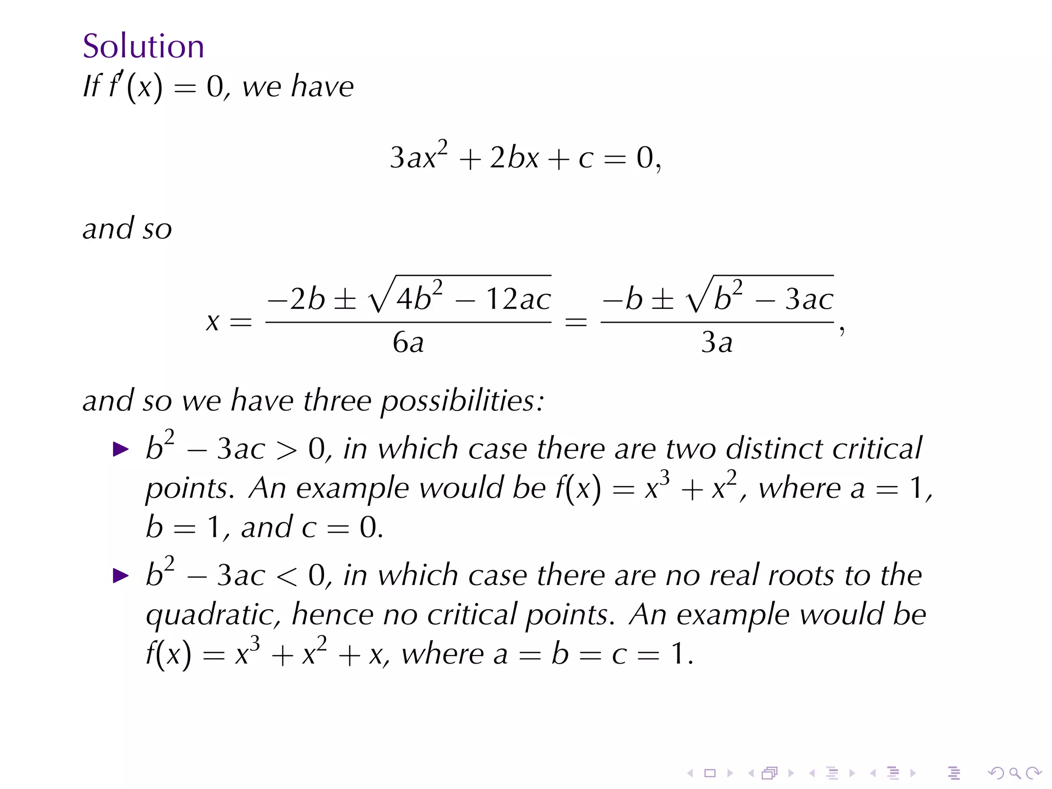
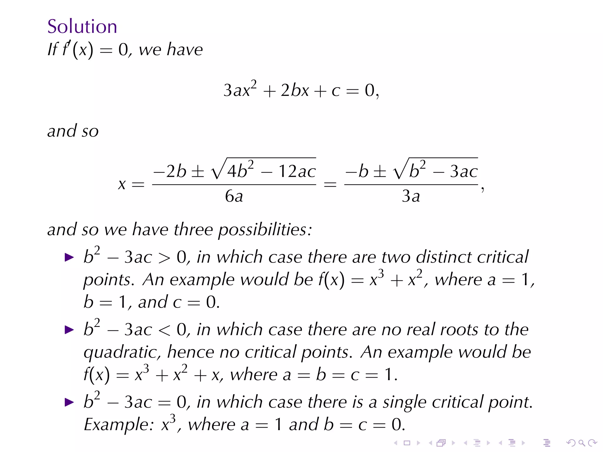
Solution
Since f′ (x) = 2, which is never zero, we have no critical points
and we need only investigate the endpoints:
f(−1) = 2(−1) − 5 = −7
f(2) = 2(2) − 5 = −1
. . . . . .](https://image.slidesharecdn.com/lesson19-maximumandminimumvalues034slides-091105142101-phpapp01/75/Lesson19-Maximum-And-Minimum-Values-034-Slides-45-2048.jpg)
![Example
Find the extreme values of f(x) = 2x − 5 on [−1, 2].
Solution
Since f′ (x) = 2, which is never zero, we have no critical points
and we need only investigate the endpoints:
f(−1) = 2(−1) − 5 = −7
f(2) = 2(2) − 5 = −1
So
The absolute minimum (point) is at −1; the minimum value
is −7.
The absolute maximum (point) is at 2; the maximum value is
−1.
. . . . . .](https://image.slidesharecdn.com/lesson19-maximumandminimumvalues034slides-091105142101-phpapp01/75/Lesson19-Maximum-And-Minimum-Values-034-Slides-46-2048.jpg)
![Example
Find the extreme values of f(x) = x2 − 1 on [−1, 2].
. . . . . .](https://image.slidesharecdn.com/lesson19-maximumandminimumvalues034slides-091105142101-phpapp01/75/Lesson19-Maximum-And-Minimum-Values-034-Slides-47-2048.jpg)
![Example
Find the extreme values of f(x) = x2 − 1 on [−1, 2].
Solution
We have f′ (x) = 2x, which is zero when x = 0.
. . . . . .](https://image.slidesharecdn.com/lesson19-maximumandminimumvalues034slides-091105142101-phpapp01/75/Lesson19-Maximum-And-Minimum-Values-034-Slides-48-2048.jpg)
![Example
Find the extreme values of f(x) = x2 − 1 on [−1, 2].
Solution
We have f′ (x) = 2x, which is zero when x = 0. So our points to
check are:
f(−1) =
f(0) =
f(2) =
. . . . . .](https://image.slidesharecdn.com/lesson19-maximumandminimumvalues034slides-091105142101-phpapp01/75/Lesson19-Maximum-And-Minimum-Values-034-Slides-49-2048.jpg)
![Example
Find the extreme values of f(x) = x2 − 1 on [−1, 2].
Solution
We have f′ (x) = 2x, which is zero when x = 0. So our points to
check are:
f(−1) = 0
f(0) =
f(2) =
. . . . . .](https://image.slidesharecdn.com/lesson19-maximumandminimumvalues034slides-091105142101-phpapp01/75/Lesson19-Maximum-And-Minimum-Values-034-Slides-50-2048.jpg)
![Example
Find the extreme values of f(x) = x2 − 1 on [−1, 2].
Solution
We have f′ (x) = 2x, which is zero when x = 0. So our points to
check are:
f(−1) = 0
f(0) = − 1
f(2) =
. . . . . .](https://image.slidesharecdn.com/lesson19-maximumandminimumvalues034slides-091105142101-phpapp01/75/Lesson19-Maximum-And-Minimum-Values-034-Slides-51-2048.jpg)
![Example
Find the extreme values of f(x) = x2 − 1 on [−1, 2].
Solution
We have f′ (x) = 2x, which is zero when x = 0. So our points to
check are:
f(−1) = 0
f(0) = − 1
f(2) = 3
. . . . . .](https://image.slidesharecdn.com/lesson19-maximumandminimumvalues034slides-091105142101-phpapp01/75/Lesson19-Maximum-And-Minimum-Values-034-Slides-52-2048.jpg)
![Example
Find the extreme values of f(x) = x2 − 1 on [−1, 2].
Solution
We have f′ (x) = 2x, which is zero when x = 0. So our points to
check are:
f(−1) = 0
f(0) = − 1 (absolute min)
f(2) = 3
. . . . . .](https://image.slidesharecdn.com/lesson19-maximumandminimumvalues034slides-091105142101-phpapp01/75/Lesson19-Maximum-And-Minimum-Values-034-Slides-53-2048.jpg)
![Example
Find the extreme values of f(x) = x2 − 1 on [−1, 2].
Solution
We have f′ (x) = 2x, which is zero when x = 0. So our points to
check are:
f(−1) = 0
f(0) = − 1 (absolute min)
f(2) = 3 (absolute max)
. . . . . .](https://image.slidesharecdn.com/lesson19-maximumandminimumvalues034slides-091105142101-phpapp01/75/Lesson19-Maximum-And-Minimum-Values-034-Slides-54-2048.jpg)
![Example
Find the extreme values of f(x) = 2x3 − 3x2 + 1 on [−1, 2].
. . . . . .](https://image.slidesharecdn.com/lesson19-maximumandminimumvalues034slides-091105142101-phpapp01/75/Lesson19-Maximum-And-Minimum-Values-034-Slides-55-2048.jpg)
![Example
Find the extreme values of f(x) = 2x3 − 3x2 + 1 on [−1, 2].
Solution
Since f′ (x) = 6x2 − 6x = 6x(x − 1), we have critical points at
x = 0 and x = 1.
. . . . . .](https://image.slidesharecdn.com/lesson19-maximumandminimumvalues034slides-091105142101-phpapp01/75/Lesson19-Maximum-And-Minimum-Values-034-Slides-56-2048.jpg)
![Example
Find the extreme values of f(x) = 2x3 − 3x2 + 1 on [−1, 2].
Solution
Since f′ (x) = 6x2 − 6x = 6x(x − 1), we have critical points at
x = 0 and x = 1. The values to check are
f(−1) =
f(0) =
f(1) =
f(2) =
. . . . . .](https://image.slidesharecdn.com/lesson19-maximumandminimumvalues034slides-091105142101-phpapp01/75/Lesson19-Maximum-And-Minimum-Values-034-Slides-57-2048.jpg)
![Example
Find the extreme values of f(x) = 2x3 − 3x2 + 1 on [−1, 2].
Solution
Since f′ (x) = 6x2 − 6x = 6x(x − 1), we have critical points at
x = 0 and x = 1. The values to check are
f(−1) = − 4
f(0) =
f(1) =
f(2) =
. . . . . .](https://image.slidesharecdn.com/lesson19-maximumandminimumvalues034slides-091105142101-phpapp01/75/Lesson19-Maximum-And-Minimum-Values-034-Slides-58-2048.jpg)
![Example
Find the extreme values of f(x) = 2x3 − 3x2 + 1 on [−1, 2].
Solution
Since f′ (x) = 6x2 − 6x = 6x(x − 1), we have critical points at
x = 0 and x = 1. The values to check are
f(−1) = − 4
f(0) = 1
f(1) =
f(2) =
. . . . . .](https://image.slidesharecdn.com/lesson19-maximumandminimumvalues034slides-091105142101-phpapp01/75/Lesson19-Maximum-And-Minimum-Values-034-Slides-59-2048.jpg)
![Example
Find the extreme values of f(x) = 2x3 − 3x2 + 1 on [−1, 2].
Solution
Since f′ (x) = 6x2 − 6x = 6x(x − 1), we have critical points at
x = 0 and x = 1. The values to check are
f(−1) = − 4
f(0) = 1
f(1) = 0
f(2) =
. . . . . .](https://image.slidesharecdn.com/lesson19-maximumandminimumvalues034slides-091105142101-phpapp01/75/Lesson19-Maximum-And-Minimum-Values-034-Slides-60-2048.jpg)
![Example
Find the extreme values of f(x) = 2x3 − 3x2 + 1 on [−1, 2].
Solution
Since f′ (x) = 6x2 − 6x = 6x(x − 1), we have critical points at
x = 0 and x = 1. The values to check are
f(−1) = − 4
f(0) = 1
f(1) = 0
f(2) = 5
. . . . . .](https://image.slidesharecdn.com/lesson19-maximumandminimumvalues034slides-091105142101-phpapp01/75/Lesson19-Maximum-And-Minimum-Values-034-Slides-61-2048.jpg)
![Example
Find the extreme values of f(x) = 2x3 − 3x2 + 1 on [−1, 2].
Solution
Since f′ (x) = 6x2 − 6x = 6x(x − 1), we have critical points at
x = 0 and x = 1. The values to check are
f(−1) = − 4 (absolute min)
f(0) = 1
f(1) = 0
f(2) = 5
. . . . . .](https://image.slidesharecdn.com/lesson19-maximumandminimumvalues034slides-091105142101-phpapp01/75/Lesson19-Maximum-And-Minimum-Values-034-Slides-62-2048.jpg)
![Example
Find the extreme values of f(x) = 2x3 − 3x2 + 1 on [−1, 2].
Solution
Since f′ (x) = 6x2 − 6x = 6x(x − 1), we have critical points at
x = 0 and x = 1. The values to check are
f(−1) = − 4 (absolute min)
f(0) = 1
f(1) = 0
f(2) = 5 (absolute max)
. . . . . .](https://image.slidesharecdn.com/lesson19-maximumandminimumvalues034slides-091105142101-phpapp01/75/Lesson19-Maximum-And-Minimum-Values-034-Slides-63-2048.jpg)
![Example
Find the extreme values of f(x) = 2x3 − 3x2 + 1 on [−1, 2].
Solution
Since f′ (x) = 6x2 − 6x = 6x(x − 1), we have critical points at
x = 0 and x = 1. The values to check are
f(−1) = − 4 (absolute min)
f(0) = 1 (local max)
f(1) = 0
f(2) = 5 (absolute max)
. . . . . .](https://image.slidesharecdn.com/lesson19-maximumandminimumvalues034slides-091105142101-phpapp01/75/Lesson19-Maximum-And-Minimum-Values-034-Slides-64-2048.jpg)
![Example
Find the extreme values of f(x) = 2x3 − 3x2 + 1 on [−1, 2].
Solution
Since f′ (x) = 6x2 − 6x = 6x(x − 1), we have critical points at
x = 0 and x = 1. The values to check are
f(−1) = − 4 (absolute min)
f(0) = 1 (local max)
f(1) = 0 (local min)
f(2) = 5 (absolute max)
. . . . . .](https://image.slidesharecdn.com/lesson19-maximumandminimumvalues034slides-091105142101-phpapp01/75/Lesson19-Maximum-And-Minimum-Values-034-Slides-65-2048.jpg)
![Example
Find the extreme values of f(x) = x2/3 (x + 2) on [−1, 2].
. . . . . .](https://image.slidesharecdn.com/lesson19-maximumandminimumvalues034slides-091105142101-phpapp01/75/Lesson19-Maximum-And-Minimum-Values-034-Slides-66-2048.jpg)
![Example
Find the extreme values of f(x) = x2/3 (x + 2) on [−1, 2].
Solution
Write f(x) = x5/3 + 2x2/3 , then
5 2/3 4 −1/3 1 −1/3
f′ (x) = x + x = x (5x + 4)
3 3 3
Thus f′ (−4/5) = 0 and f is not differentiable at 0.
. . . . . .](https://image.slidesharecdn.com/lesson19-maximumandminimumvalues034slides-091105142101-phpapp01/75/Lesson19-Maximum-And-Minimum-Values-034-Slides-67-2048.jpg)
![Example
Find the extreme values of f(x) = x2/3 (x + 2) on [−1, 2].
Solution
Write f(x) = x5/3 + 2x2/3 , then
5 2/3 4 −1/3 1 −1/3
f′ (x) = x + x = x (5x + 4)
3 3 3
Thus f′ (−4/5) = 0 and f is not differentiable at 0. So our points to
check are:
f(−1) =
f(−4/5) =
f(0) =
f(2) =
. . . . . .](https://image.slidesharecdn.com/lesson19-maximumandminimumvalues034slides-091105142101-phpapp01/75/Lesson19-Maximum-And-Minimum-Values-034-Slides-68-2048.jpg)
![Example
Find the extreme values of f(x) = x2/3 (x + 2) on [−1, 2].
Solution
Write f(x) = x5/3 + 2x2/3 , then
5 2/3 4 −1/3 1 −1/3
f′ (x) = x + x = x (5x + 4)
3 3 3
Thus f′ (−4/5) = 0 and f is not differentiable at 0. So our points to
check are:
f(−1) = 1
f(−4/5) =
f(0) =
f(2) =
. . . . . .](https://image.slidesharecdn.com/lesson19-maximumandminimumvalues034slides-091105142101-phpapp01/75/Lesson19-Maximum-And-Minimum-Values-034-Slides-69-2048.jpg)
![Example
Find the extreme values of f(x) = x2/3 (x + 2) on [−1, 2].
Solution
Write f(x) = x5/3 + 2x2/3 , then
5 2/3 4 −1/3 1 −1/3
f′ (x) = x + x = x (5x + 4)
3 3 3
Thus f′ (−4/5) = 0 and f is not differentiable at 0. So our points to
check are:
f(−1) = 1
f(−4/5) = 1.0341
f(0) =
f(2) =
. . . . . .](https://image.slidesharecdn.com/lesson19-maximumandminimumvalues034slides-091105142101-phpapp01/75/Lesson19-Maximum-And-Minimum-Values-034-Slides-70-2048.jpg)
![Example
Find the extreme values of f(x) = x2/3 (x + 2) on [−1, 2].
Solution
Write f(x) = x5/3 + 2x2/3 , then
5 2/3 4 −1/3 1 −1/3
f′ (x) = x + x = x (5x + 4)
3 3 3
Thus f′ (−4/5) = 0 and f is not differentiable at 0. So our points to
check are:
f(−1) = 1
f(−4/5) = 1.0341
f(0) = 0
f(2) =
. . . . . .](https://image.slidesharecdn.com/lesson19-maximumandminimumvalues034slides-091105142101-phpapp01/75/Lesson19-Maximum-And-Minimum-Values-034-Slides-71-2048.jpg)
![Example
Find the extreme values of f(x) = x2/3 (x + 2) on [−1, 2].
Solution
Write f(x) = x5/3 + 2x2/3 , then
5 2/3 4 −1/3 1 −1/3
f′ (x) = x + x = x (5x + 4)
3 3 3
Thus f′ (−4/5) = 0 and f is not differentiable at 0. So our points to
check are:
f(−1) = 1
f(−4/5) = 1.0341
f(0) = 0
f(2) = 6.3496
. . . . . .](https://image.slidesharecdn.com/lesson19-maximumandminimumvalues034slides-091105142101-phpapp01/75/Lesson19-Maximum-And-Minimum-Values-034-Slides-72-2048.jpg)
![Example
Find the extreme values of f(x) = x2/3 (x + 2) on [−1, 2].
Solution
Write f(x) = x5/3 + 2x2/3 , then
5 2/3 4 −1/3 1 −1/3
f′ (x) = x + x = x (5x + 4)
3 3 3
Thus f′ (−4/5) = 0 and f is not differentiable at 0. So our points to
check are:
f(−1) = 1
f(−4/5) = 1.0341
f(0) = 0 (absolute min)
f(2) = 6.3496
. . . . . .](https://image.slidesharecdn.com/lesson19-maximumandminimumvalues034slides-091105142101-phpapp01/75/Lesson19-Maximum-And-Minimum-Values-034-Slides-73-2048.jpg)
![Example
Find the extreme values of f(x) = x2/3 (x + 2) on [−1, 2].
Solution
Write f(x) = x5/3 + 2x2/3 , then
5 2/3 4 −1/3 1 −1/3
f′ (x) = x + x = x (5x + 4)
3 3 3
Thus f′ (−4/5) = 0 and f is not differentiable at 0. So our points to
check are:
f(−1) = 1
f(−4/5) = 1.0341
f(0) = 0 (absolute min)
f(2) = 6.3496 (absolute max)
. . . . . .](https://image.slidesharecdn.com/lesson19-maximumandminimumvalues034slides-091105142101-phpapp01/75/Lesson19-Maximum-And-Minimum-Values-034-Slides-74-2048.jpg)
![Example
Find the extreme values of f(x) = x2/3 (x + 2) on [−1, 2].
Solution
Write f(x) = x5/3 + 2x2/3 , then
5 2/3 4 −1/3 1 −1/3
f′ (x) = x + x = x (5x + 4)
3 3 3
Thus f′ (−4/5) = 0 and f is not differentiable at 0. So our points to
check are:
f(−1) = 1
f(−4/5) = 1.0341 (relative max)
f(0) = 0 (absolute min)
f(2) = 6.3496 (absolute max)
. . . . . .](https://image.slidesharecdn.com/lesson19-maximumandminimumvalues034slides-091105142101-phpapp01/75/Lesson19-Maximum-And-Minimum-Values-034-Slides-75-2048.jpg)
![Example √
Find the extreme values of f(x) = 4 − x2 on [−2, 1].
. . . . . .](https://image.slidesharecdn.com/lesson19-maximumandminimumvalues034slides-091105142101-phpapp01/75/Lesson19-Maximum-And-Minimum-Values-034-Slides-76-2048.jpg)
![Example √
Find the extreme values of f(x) = 4 − x2 on [−2, 1].
Solution
x
We have f′ (x) = − √ , which is zero when x = 0. (f is not
4 − x2
differentiable at ±2 as well.)
. . . . . .](https://image.slidesharecdn.com/lesson19-maximumandminimumvalues034slides-091105142101-phpapp01/75/Lesson19-Maximum-And-Minimum-Values-034-Slides-77-2048.jpg)
![Example √
Find the extreme values of f(x) = 4 − x2 on [−2, 1].
Solution
x
We have f′ (x) = − √ , which is zero when x = 0. (f is not
4 − x2
differentiable at ±2 as well.) So our points to check are:
f(−2) =
f(0) =
f(1) =
. . . . . .](https://image.slidesharecdn.com/lesson19-maximumandminimumvalues034slides-091105142101-phpapp01/75/Lesson19-Maximum-And-Minimum-Values-034-Slides-78-2048.jpg)
![Example √
Find the extreme values of f(x) = 4 − x2 on [−2, 1].
Solution
x
We have f′ (x) = − √ , which is zero when x = 0. (f is not
4 − x2
differentiable at ±2 as well.) So our points to check are:
f(−2) = 0
f(0) =
f(1) =
. . . . . .](https://image.slidesharecdn.com/lesson19-maximumandminimumvalues034slides-091105142101-phpapp01/75/Lesson19-Maximum-And-Minimum-Values-034-Slides-79-2048.jpg)
![Example √
Find the extreme values of f(x) = 4 − x2 on [−2, 1].
Solution
x
We have f′ (x) = − √ , which is zero when x = 0. (f is not
4 − x2
differentiable at ±2 as well.) So our points to check are:
f(−2) = 0
f(0) = 2
f(1) =
. . . . . .](https://image.slidesharecdn.com/lesson19-maximumandminimumvalues034slides-091105142101-phpapp01/75/Lesson19-Maximum-And-Minimum-Values-034-Slides-80-2048.jpg)
![Example √
Find the extreme values of f(x) = 4 − x2 on [−2, 1].
Solution
x
We have f′ (x) = − √ , which is zero when x = 0. (f is not
4 − x2
differentiable at ±2 as well.) So our points to check are:
f(−2) = 0
f(0) = 2
√
f(1) = 3
. . . . . .](https://image.slidesharecdn.com/lesson19-maximumandminimumvalues034slides-091105142101-phpapp01/75/Lesson19-Maximum-And-Minimum-Values-034-Slides-81-2048.jpg)
![Example √
Find the extreme values of f(x) = 4 − x2 on [−2, 1].
Solution
x
We have f′ (x) = − √ , which is zero when x = 0. (f is not
4 − x2
differentiable at ±2 as well.) So our points to check are:
f(−2) = 0 (absolute min)
f(0) = 2
√
f(1) = 3
. . . . . .](https://image.slidesharecdn.com/lesson19-maximumandminimumvalues034slides-091105142101-phpapp01/75/Lesson19-Maximum-And-Minimum-Values-034-Slides-82-2048.jpg)
![Example √
Find the extreme values of f(x) = 4 − x2 on [−2, 1].
Solution
x
We have f′ (x) = − √ , which is zero when x = 0. (f is not
4 − x2
differentiable at ±2 as well.) So our points to check are:
f(−2) = 0 (absolute min)
f(0) = 2 (absolute max)
√
f(1) = 3
. . . . . .](https://image.slidesharecdn.com/lesson19-maximumandminimumvalues034slides-091105142101-phpapp01/75/Lesson19-Maximum-And-Minimum-Values-034-Slides-83-2048.jpg)


![Theorem (The Extreme Value Theorem)
Let f be a function which is continuous on the closed interval
[a, b]. Then f attains an absolute maximum value f(c) and an
absolute minimum value f(d) at numbers c and d in [a, b].
. . . . . .](https://crownmelresort.com/image.slidesharecdn.com/lesson19-maximumandminimumvalues034slides-091105142101-phpapp01/75/Lesson19-Maximum-And-Minimum-Values-034-Slides-13-2048.jpg)
![Theorem (The Extreme Value Theorem)
Let f be a function which is continuous on the closed interval
[a, b]. Then f attains an absolute maximum value f(c) and an
absolute minimum value f(d) at numbers c and d in [a, b].
.
.
. .
a
. b
.
. . . . . .](https://crownmelresort.com/image.slidesharecdn.com/lesson19-maximumandminimumvalues034slides-091105142101-phpapp01/75/Lesson19-Maximum-And-Minimum-Values-034-Slides-14-2048.jpg)
![Theorem (The Extreme Value Theorem)
Let f be a function which is continuous on the closed interval
[a, b]. Then f attains an absolute maximum value f(c) and an
absolute minimum value f(d) at numbers c and d in [a, b].
.
maximum .(c)
f
.
value
. .
minimum .(d)
f
.
value
. . ..
a
. d c
b
.
minimum maximum
. . . . . .](https://crownmelresort.com/image.slidesharecdn.com/lesson19-maximumandminimumvalues034slides-091105142101-phpapp01/75/Lesson19-Maximum-And-Minimum-Values-034-Slides-15-2048.jpg)


![Bad Example #1
Example
Consider the function .
{
x 0≤x<1
f (x ) = . .
| .
x − 2 1 ≤ x ≤ 2. 1
.
.
Then although values of f(x) get arbitrarily close to 1 and never
bigger than 1, 1 is not the maximum value of f on [0, 1] because
it is never achieved.
. . . . . .](https://crownmelresort.com/image.slidesharecdn.com/lesson19-maximumandminimumvalues034slides-091105142101-phpapp01/75/Lesson19-Maximum-And-Minimum-Values-034-Slides-19-2048.jpg)


![Flowchart for placing extrema
Thanks to Fermat
Suppose f is a continuous function on the closed, bounded
interval [a, b], and c is a global maximum point.
.
. . c is a
start
local max
. . .
Is c an Is f diff’ble f is not
n
.o n
.o
endpoint? at c? diff at c
y
. es y
. es
. c = a or .
f′ (c) = 0
c = b
. . . . . .](https://crownmelresort.com/image.slidesharecdn.com/lesson19-maximumandminimumvalues034slides-091105142101-phpapp01/75/Lesson19-Maximum-And-Minimum-Values-034-Slides-41-2048.jpg)
![The Closed Interval Method
This means to find the maximum value of f on [a, b], we need to:
Evaluate f at the endpoints a and b
Evaluate f at the critical points or critical numbers x where
either f′ (x) = 0 or f is not differentiable at x.
The points with the largest function value are the global
maximum points
The points with the smallest or most negative function value
are the global minimum points.
. . . . . .](https://crownmelresort.com/image.slidesharecdn.com/lesson19-maximumandminimumvalues034slides-091105142101-phpapp01/75/Lesson19-Maximum-And-Minimum-Values-034-Slides-42-2048.jpg)

![Example
Find the extreme values of f(x) = 2x − 5 on [−1, 2].
. . . . . .](https://crownmelresort.com/image.slidesharecdn.com/lesson19-maximumandminimumvalues034slides-091105142101-phpapp01/75/Lesson19-Maximum-And-Minimum-Values-034-Slides-44-2048.jpg)
![Example
Find the extreme values of f(x) = 2x − 5 on [−1, 2].
Solution
Since f′ (x) = 2, which is never zero, we have no critical points
and we need only investigate the endpoints:
f(−1) = 2(−1) − 5 = −7
f(2) = 2(2) − 5 = −1
. . . . . .](https://crownmelresort.com/image.slidesharecdn.com/lesson19-maximumandminimumvalues034slides-091105142101-phpapp01/75/Lesson19-Maximum-And-Minimum-Values-034-Slides-45-2048.jpg)
![Example
Find the extreme values of f(x) = 2x − 5 on [−1, 2].
Solution
Since f′ (x) = 2, which is never zero, we have no critical points
and we need only investigate the endpoints:
f(−1) = 2(−1) − 5 = −7
f(2) = 2(2) − 5 = −1
So
The absolute minimum (point) is at −1; the minimum value
is −7.
The absolute maximum (point) is at 2; the maximum value is
−1.
. . . . . .](https://crownmelresort.com/image.slidesharecdn.com/lesson19-maximumandminimumvalues034slides-091105142101-phpapp01/75/Lesson19-Maximum-And-Minimum-Values-034-Slides-46-2048.jpg)
![Example
Find the extreme values of f(x) = x2 − 1 on [−1, 2].
. . . . . .](https://crownmelresort.com/image.slidesharecdn.com/lesson19-maximumandminimumvalues034slides-091105142101-phpapp01/75/Lesson19-Maximum-And-Minimum-Values-034-Slides-47-2048.jpg)
![Example
Find the extreme values of f(x) = x2 − 1 on [−1, 2].
Solution
We have f′ (x) = 2x, which is zero when x = 0.
. . . . . .](https://crownmelresort.com/image.slidesharecdn.com/lesson19-maximumandminimumvalues034slides-091105142101-phpapp01/75/Lesson19-Maximum-And-Minimum-Values-034-Slides-48-2048.jpg)
![Example
Find the extreme values of f(x) = x2 − 1 on [−1, 2].
Solution
We have f′ (x) = 2x, which is zero when x = 0. So our points to
check are:
f(−1) =
f(0) =
f(2) =
. . . . . .](https://crownmelresort.com/image.slidesharecdn.com/lesson19-maximumandminimumvalues034slides-091105142101-phpapp01/75/Lesson19-Maximum-And-Minimum-Values-034-Slides-49-2048.jpg)
![Example
Find the extreme values of f(x) = x2 − 1 on [−1, 2].
Solution
We have f′ (x) = 2x, which is zero when x = 0. So our points to
check are:
f(−1) = 0
f(0) =
f(2) =
. . . . . .](https://crownmelresort.com/image.slidesharecdn.com/lesson19-maximumandminimumvalues034slides-091105142101-phpapp01/75/Lesson19-Maximum-And-Minimum-Values-034-Slides-50-2048.jpg)
![Example
Find the extreme values of f(x) = x2 − 1 on [−1, 2].
Solution
We have f′ (x) = 2x, which is zero when x = 0. So our points to
check are:
f(−1) = 0
f(0) = − 1
f(2) =
. . . . . .](https://crownmelresort.com/image.slidesharecdn.com/lesson19-maximumandminimumvalues034slides-091105142101-phpapp01/75/Lesson19-Maximum-And-Minimum-Values-034-Slides-51-2048.jpg)
![Example
Find the extreme values of f(x) = x2 − 1 on [−1, 2].
Solution
We have f′ (x) = 2x, which is zero when x = 0. So our points to
check are:
f(−1) = 0
f(0) = − 1
f(2) = 3
. . . . . .](https://crownmelresort.com/image.slidesharecdn.com/lesson19-maximumandminimumvalues034slides-091105142101-phpapp01/75/Lesson19-Maximum-And-Minimum-Values-034-Slides-52-2048.jpg)
![Example
Find the extreme values of f(x) = x2 − 1 on [−1, 2].
Solution
We have f′ (x) = 2x, which is zero when x = 0. So our points to
check are:
f(−1) = 0
f(0) = − 1 (absolute min)
f(2) = 3
. . . . . .](https://crownmelresort.com/image.slidesharecdn.com/lesson19-maximumandminimumvalues034slides-091105142101-phpapp01/75/Lesson19-Maximum-And-Minimum-Values-034-Slides-53-2048.jpg)
![Example
Find the extreme values of f(x) = x2 − 1 on [−1, 2].
Solution
We have f′ (x) = 2x, which is zero when x = 0. So our points to
check are:
f(−1) = 0
f(0) = − 1 (absolute min)
f(2) = 3 (absolute max)
. . . . . .](https://crownmelresort.com/image.slidesharecdn.com/lesson19-maximumandminimumvalues034slides-091105142101-phpapp01/75/Lesson19-Maximum-And-Minimum-Values-034-Slides-54-2048.jpg)
![Example
Find the extreme values of f(x) = 2x3 − 3x2 + 1 on [−1, 2].
. . . . . .](https://crownmelresort.com/image.slidesharecdn.com/lesson19-maximumandminimumvalues034slides-091105142101-phpapp01/75/Lesson19-Maximum-And-Minimum-Values-034-Slides-55-2048.jpg)
![Example
Find the extreme values of f(x) = 2x3 − 3x2 + 1 on [−1, 2].
Solution
Since f′ (x) = 6x2 − 6x = 6x(x − 1), we have critical points at
x = 0 and x = 1.
. . . . . .](https://crownmelresort.com/image.slidesharecdn.com/lesson19-maximumandminimumvalues034slides-091105142101-phpapp01/75/Lesson19-Maximum-And-Minimum-Values-034-Slides-56-2048.jpg)
![Example
Find the extreme values of f(x) = 2x3 − 3x2 + 1 on [−1, 2].
Solution
Since f′ (x) = 6x2 − 6x = 6x(x − 1), we have critical points at
x = 0 and x = 1. The values to check are
f(−1) =
f(0) =
f(1) =
f(2) =
. . . . . .](https://crownmelresort.com/image.slidesharecdn.com/lesson19-maximumandminimumvalues034slides-091105142101-phpapp01/75/Lesson19-Maximum-And-Minimum-Values-034-Slides-57-2048.jpg)
![Example
Find the extreme values of f(x) = 2x3 − 3x2 + 1 on [−1, 2].
Solution
Since f′ (x) = 6x2 − 6x = 6x(x − 1), we have critical points at
x = 0 and x = 1. The values to check are
f(−1) = − 4
f(0) =
f(1) =
f(2) =
. . . . . .](https://crownmelresort.com/image.slidesharecdn.com/lesson19-maximumandminimumvalues034slides-091105142101-phpapp01/75/Lesson19-Maximum-And-Minimum-Values-034-Slides-58-2048.jpg)
![Example
Find the extreme values of f(x) = 2x3 − 3x2 + 1 on [−1, 2].
Solution
Since f′ (x) = 6x2 − 6x = 6x(x − 1), we have critical points at
x = 0 and x = 1. The values to check are
f(−1) = − 4
f(0) = 1
f(1) =
f(2) =
. . . . . .](https://crownmelresort.com/image.slidesharecdn.com/lesson19-maximumandminimumvalues034slides-091105142101-phpapp01/75/Lesson19-Maximum-And-Minimum-Values-034-Slides-59-2048.jpg)
![Example
Find the extreme values of f(x) = 2x3 − 3x2 + 1 on [−1, 2].
Solution
Since f′ (x) = 6x2 − 6x = 6x(x − 1), we have critical points at
x = 0 and x = 1. The values to check are
f(−1) = − 4
f(0) = 1
f(1) = 0
f(2) =
. . . . . .](https://crownmelresort.com/image.slidesharecdn.com/lesson19-maximumandminimumvalues034slides-091105142101-phpapp01/75/Lesson19-Maximum-And-Minimum-Values-034-Slides-60-2048.jpg)
![Example
Find the extreme values of f(x) = 2x3 − 3x2 + 1 on [−1, 2].
Solution
Since f′ (x) = 6x2 − 6x = 6x(x − 1), we have critical points at
x = 0 and x = 1. The values to check are
f(−1) = − 4
f(0) = 1
f(1) = 0
f(2) = 5
. . . . . .](https://crownmelresort.com/image.slidesharecdn.com/lesson19-maximumandminimumvalues034slides-091105142101-phpapp01/75/Lesson19-Maximum-And-Minimum-Values-034-Slides-61-2048.jpg)
![Example
Find the extreme values of f(x) = 2x3 − 3x2 + 1 on [−1, 2].
Solution
Since f′ (x) = 6x2 − 6x = 6x(x − 1), we have critical points at
x = 0 and x = 1. The values to check are
f(−1) = − 4 (absolute min)
f(0) = 1
f(1) = 0
f(2) = 5
. . . . . .](https://crownmelresort.com/image.slidesharecdn.com/lesson19-maximumandminimumvalues034slides-091105142101-phpapp01/75/Lesson19-Maximum-And-Minimum-Values-034-Slides-62-2048.jpg)
![Example
Find the extreme values of f(x) = 2x3 − 3x2 + 1 on [−1, 2].
Solution
Since f′ (x) = 6x2 − 6x = 6x(x − 1), we have critical points at
x = 0 and x = 1. The values to check are
f(−1) = − 4 (absolute min)
f(0) = 1
f(1) = 0
f(2) = 5 (absolute max)
. . . . . .](https://crownmelresort.com/image.slidesharecdn.com/lesson19-maximumandminimumvalues034slides-091105142101-phpapp01/75/Lesson19-Maximum-And-Minimum-Values-034-Slides-63-2048.jpg)
![Example
Find the extreme values of f(x) = 2x3 − 3x2 + 1 on [−1, 2].
Solution
Since f′ (x) = 6x2 − 6x = 6x(x − 1), we have critical points at
x = 0 and x = 1. The values to check are
f(−1) = − 4 (absolute min)
f(0) = 1 (local max)
f(1) = 0
f(2) = 5 (absolute max)
. . . . . .](https://crownmelresort.com/image.slidesharecdn.com/lesson19-maximumandminimumvalues034slides-091105142101-phpapp01/75/Lesson19-Maximum-And-Minimum-Values-034-Slides-64-2048.jpg)
![Example
Find the extreme values of f(x) = 2x3 − 3x2 + 1 on [−1, 2].
Solution
Since f′ (x) = 6x2 − 6x = 6x(x − 1), we have critical points at
x = 0 and x = 1. The values to check are
f(−1) = − 4 (absolute min)
f(0) = 1 (local max)
f(1) = 0 (local min)
f(2) = 5 (absolute max)
. . . . . .](https://crownmelresort.com/image.slidesharecdn.com/lesson19-maximumandminimumvalues034slides-091105142101-phpapp01/75/Lesson19-Maximum-And-Minimum-Values-034-Slides-65-2048.jpg)
![Example
Find the extreme values of f(x) = x2/3 (x + 2) on [−1, 2].
. . . . . .](https://crownmelresort.com/image.slidesharecdn.com/lesson19-maximumandminimumvalues034slides-091105142101-phpapp01/75/Lesson19-Maximum-And-Minimum-Values-034-Slides-66-2048.jpg)
![Example
Find the extreme values of f(x) = x2/3 (x + 2) on [−1, 2].
Solution
Write f(x) = x5/3 + 2x2/3 , then
5 2/3 4 −1/3 1 −1/3
f′ (x) = x + x = x (5x + 4)
3 3 3
Thus f′ (−4/5) = 0 and f is not differentiable at 0.
. . . . . .](https://crownmelresort.com/image.slidesharecdn.com/lesson19-maximumandminimumvalues034slides-091105142101-phpapp01/75/Lesson19-Maximum-And-Minimum-Values-034-Slides-67-2048.jpg)
![Example
Find the extreme values of f(x) = x2/3 (x + 2) on [−1, 2].
Solution
Write f(x) = x5/3 + 2x2/3 , then
5 2/3 4 −1/3 1 −1/3
f′ (x) = x + x = x (5x + 4)
3 3 3
Thus f′ (−4/5) = 0 and f is not differentiable at 0. So our points to
check are:
f(−1) =
f(−4/5) =
f(0) =
f(2) =
. . . . . .](https://crownmelresort.com/image.slidesharecdn.com/lesson19-maximumandminimumvalues034slides-091105142101-phpapp01/75/Lesson19-Maximum-And-Minimum-Values-034-Slides-68-2048.jpg)
![Example
Find the extreme values of f(x) = x2/3 (x + 2) on [−1, 2].
Solution
Write f(x) = x5/3 + 2x2/3 , then
5 2/3 4 −1/3 1 −1/3
f′ (x) = x + x = x (5x + 4)
3 3 3
Thus f′ (−4/5) = 0 and f is not differentiable at 0. So our points to
check are:
f(−1) = 1
f(−4/5) =
f(0) =
f(2) =
. . . . . .](https://crownmelresort.com/image.slidesharecdn.com/lesson19-maximumandminimumvalues034slides-091105142101-phpapp01/75/Lesson19-Maximum-And-Minimum-Values-034-Slides-69-2048.jpg)
![Example
Find the extreme values of f(x) = x2/3 (x + 2) on [−1, 2].
Solution
Write f(x) = x5/3 + 2x2/3 , then
5 2/3 4 −1/3 1 −1/3
f′ (x) = x + x = x (5x + 4)
3 3 3
Thus f′ (−4/5) = 0 and f is not differentiable at 0. So our points to
check are:
f(−1) = 1
f(−4/5) = 1.0341
f(0) =
f(2) =
. . . . . .](https://crownmelresort.com/image.slidesharecdn.com/lesson19-maximumandminimumvalues034slides-091105142101-phpapp01/75/Lesson19-Maximum-And-Minimum-Values-034-Slides-70-2048.jpg)
![Example
Find the extreme values of f(x) = x2/3 (x + 2) on [−1, 2].
Solution
Write f(x) = x5/3 + 2x2/3 , then
5 2/3 4 −1/3 1 −1/3
f′ (x) = x + x = x (5x + 4)
3 3 3
Thus f′ (−4/5) = 0 and f is not differentiable at 0. So our points to
check are:
f(−1) = 1
f(−4/5) = 1.0341
f(0) = 0
f(2) =
. . . . . .](https://crownmelresort.com/image.slidesharecdn.com/lesson19-maximumandminimumvalues034slides-091105142101-phpapp01/75/Lesson19-Maximum-And-Minimum-Values-034-Slides-71-2048.jpg)
![Example
Find the extreme values of f(x) = x2/3 (x + 2) on [−1, 2].
Solution
Write f(x) = x5/3 + 2x2/3 , then
5 2/3 4 −1/3 1 −1/3
f′ (x) = x + x = x (5x + 4)
3 3 3
Thus f′ (−4/5) = 0 and f is not differentiable at 0. So our points to
check are:
f(−1) = 1
f(−4/5) = 1.0341
f(0) = 0
f(2) = 6.3496
. . . . . .](https://crownmelresort.com/image.slidesharecdn.com/lesson19-maximumandminimumvalues034slides-091105142101-phpapp01/75/Lesson19-Maximum-And-Minimum-Values-034-Slides-72-2048.jpg)
![Example
Find the extreme values of f(x) = x2/3 (x + 2) on [−1, 2].
Solution
Write f(x) = x5/3 + 2x2/3 , then
5 2/3 4 −1/3 1 −1/3
f′ (x) = x + x = x (5x + 4)
3 3 3
Thus f′ (−4/5) = 0 and f is not differentiable at 0. So our points to
check are:
f(−1) = 1
f(−4/5) = 1.0341
f(0) = 0 (absolute min)
f(2) = 6.3496
. . . . . .](https://crownmelresort.com/image.slidesharecdn.com/lesson19-maximumandminimumvalues034slides-091105142101-phpapp01/75/Lesson19-Maximum-And-Minimum-Values-034-Slides-73-2048.jpg)
![Example
Find the extreme values of f(x) = x2/3 (x + 2) on [−1, 2].
Solution
Write f(x) = x5/3 + 2x2/3 , then
5 2/3 4 −1/3 1 −1/3
f′ (x) = x + x = x (5x + 4)
3 3 3
Thus f′ (−4/5) = 0 and f is not differentiable at 0. So our points to
check are:
f(−1) = 1
f(−4/5) = 1.0341
f(0) = 0 (absolute min)
f(2) = 6.3496 (absolute max)
. . . . . .](https://crownmelresort.com/image.slidesharecdn.com/lesson19-maximumandminimumvalues034slides-091105142101-phpapp01/75/Lesson19-Maximum-And-Minimum-Values-034-Slides-74-2048.jpg)
![Example
Find the extreme values of f(x) = x2/3 (x + 2) on [−1, 2].
Solution
Write f(x) = x5/3 + 2x2/3 , then
5 2/3 4 −1/3 1 −1/3
f′ (x) = x + x = x (5x + 4)
3 3 3
Thus f′ (−4/5) = 0 and f is not differentiable at 0. So our points to
check are:
f(−1) = 1
f(−4/5) = 1.0341 (relative max)
f(0) = 0 (absolute min)
f(2) = 6.3496 (absolute max)
. . . . . .](https://crownmelresort.com/image.slidesharecdn.com/lesson19-maximumandminimumvalues034slides-091105142101-phpapp01/75/Lesson19-Maximum-And-Minimum-Values-034-Slides-75-2048.jpg)
![Example √
Find the extreme values of f(x) = 4 − x2 on [−2, 1].
. . . . . .](https://crownmelresort.com/image.slidesharecdn.com/lesson19-maximumandminimumvalues034slides-091105142101-phpapp01/75/Lesson19-Maximum-And-Minimum-Values-034-Slides-76-2048.jpg)
![Example √
Find the extreme values of f(x) = 4 − x2 on [−2, 1].
Solution
x
We have f′ (x) = − √ , which is zero when x = 0. (f is not
4 − x2
differentiable at ±2 as well.)
. . . . . .](https://crownmelresort.com/image.slidesharecdn.com/lesson19-maximumandminimumvalues034slides-091105142101-phpapp01/75/Lesson19-Maximum-And-Minimum-Values-034-Slides-77-2048.jpg)
![Example √
Find the extreme values of f(x) = 4 − x2 on [−2, 1].
Solution
x
We have f′ (x) = − √ , which is zero when x = 0. (f is not
4 − x2
differentiable at ±2 as well.) So our points to check are:
f(−2) =
f(0) =
f(1) =
. . . . . .](https://crownmelresort.com/image.slidesharecdn.com/lesson19-maximumandminimumvalues034slides-091105142101-phpapp01/75/Lesson19-Maximum-And-Minimum-Values-034-Slides-78-2048.jpg)
![Example √
Find the extreme values of f(x) = 4 − x2 on [−2, 1].
Solution
x
We have f′ (x) = − √ , which is zero when x = 0. (f is not
4 − x2
differentiable at ±2 as well.) So our points to check are:
f(−2) = 0
f(0) =
f(1) =
. . . . . .](https://crownmelresort.com/image.slidesharecdn.com/lesson19-maximumandminimumvalues034slides-091105142101-phpapp01/75/Lesson19-Maximum-And-Minimum-Values-034-Slides-79-2048.jpg)
![Example √
Find the extreme values of f(x) = 4 − x2 on [−2, 1].
Solution
x
We have f′ (x) = − √ , which is zero when x = 0. (f is not
4 − x2
differentiable at ±2 as well.) So our points to check are:
f(−2) = 0
f(0) = 2
f(1) =
. . . . . .](https://crownmelresort.com/image.slidesharecdn.com/lesson19-maximumandminimumvalues034slides-091105142101-phpapp01/75/Lesson19-Maximum-And-Minimum-Values-034-Slides-80-2048.jpg)
![Example √
Find the extreme values of f(x) = 4 − x2 on [−2, 1].
Solution
x
We have f′ (x) = − √ , which is zero when x = 0. (f is not
4 − x2
differentiable at ±2 as well.) So our points to check are:
f(−2) = 0
f(0) = 2
√
f(1) = 3
. . . . . .](https://crownmelresort.com/image.slidesharecdn.com/lesson19-maximumandminimumvalues034slides-091105142101-phpapp01/75/Lesson19-Maximum-And-Minimum-Values-034-Slides-81-2048.jpg)
![Example √
Find the extreme values of f(x) = 4 − x2 on [−2, 1].
Solution
x
We have f′ (x) = − √ , which is zero when x = 0. (f is not
4 − x2
differentiable at ±2 as well.) So our points to check are:
f(−2) = 0 (absolute min)
f(0) = 2
√
f(1) = 3
. . . . . .](https://crownmelresort.com/image.slidesharecdn.com/lesson19-maximumandminimumvalues034slides-091105142101-phpapp01/75/Lesson19-Maximum-And-Minimum-Values-034-Slides-82-2048.jpg)
![Example √
Find the extreme values of f(x) = 4 − x2 on [−2, 1].
Solution
x
We have f′ (x) = − √ , which is zero when x = 0. (f is not
4 − x2
differentiable at ±2 as well.) So our points to check are:
f(−2) = 0 (absolute min)
f(0) = 2 (absolute max)
√
f(1) = 3
. . . . . .](https://crownmelresort.com/image.slidesharecdn.com/lesson19-maximumandminimumvalues034slides-091105142101-phpapp01/75/Lesson19-Maximum-And-Minimum-Values-034-Slides-83-2048.jpg)


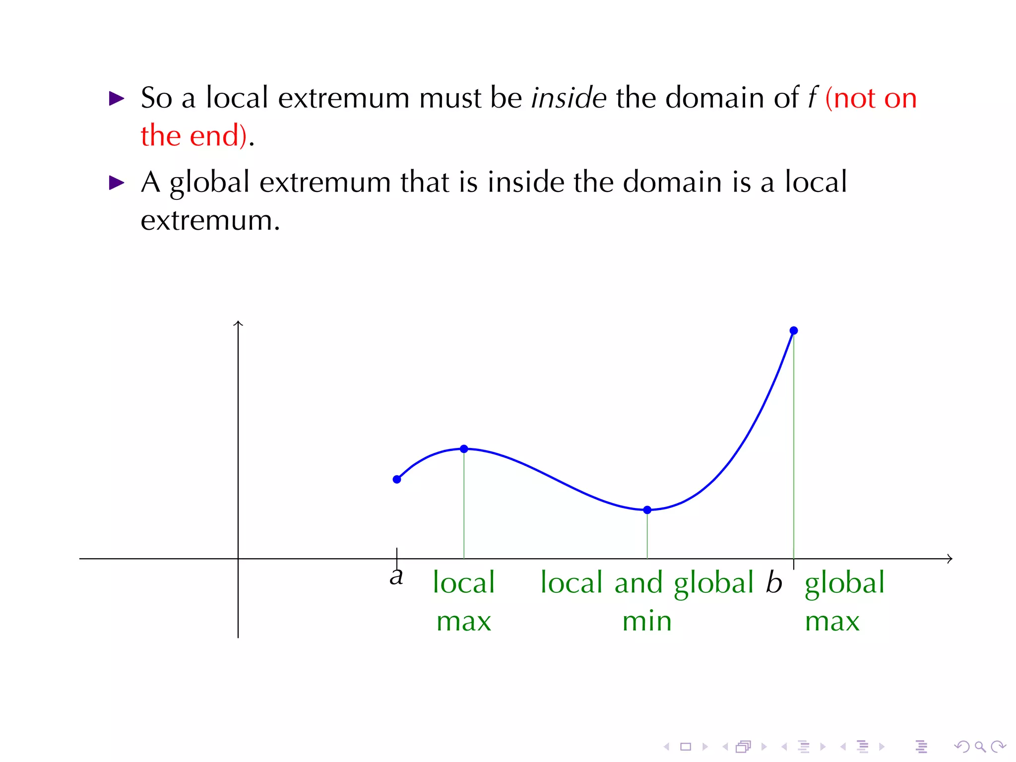
The document discusses the Extreme Value Theorem, which states that a continuous function on a closed interval [a, b] attains both an absolute maximum and minimum. It also covers definitions of local and global extrema, illustrates how to find extreme values using various examples, and references Fermat's Theorem and its implications. Additionally, it highlights the importance of identifying critical points and evaluating endpoints to determine extrema in a function.