Downloaded 1,151 times
![Features are the Keys
SIFT [Loewe IJCV 04] HOG [Dalal and Triggs CVPR 05]
SPM [Lazebnik et al. CVPR 06] DPM [Felzenszwalb et al. PAMI 10]
Color Descriptor [Van De Sande et al. PAMI 10]](https://image.slidesharecdn.com/lecture29-convolutionalneuralnetworks-visionspring2015-150504114140-conversion-gate02/75/Lecture-29-Convolutional-Neural-Networks-Computer-Vision-Spring2015-6-2048.jpg)


![Neocognitron [Fukushima, Biological Cybernetics 1980]](https://image.slidesharecdn.com/lecture29-convolutionalneuralnetworks-visionspring2015-150504114140-conversion-gate02/75/Lecture-29-Convolutional-Neural-Networks-Computer-Vision-Spring2015-14-2048.jpg)
![LeNet [LeCun et al. 1998]
Gradient-based learning applied to document
recognition [LeCun, Bottou, Bengio, Haffner 1998]](https://image.slidesharecdn.com/lecture29-convolutionalneuralnetworks-visionspring2015-150504114140-conversion-gate02/75/Lecture-29-Convolutional-Neural-Networks-Computer-Vision-Spring2015-15-2048.jpg)


![SIFT Descriptor
Image
Pixels
Apply gradient
filters
Spatial pool
(Sum)
Normalize to unit
length
Feature
Vector
Lowe [IJCV 2004]](https://image.slidesharecdn.com/lecture29-convolutionalneuralnetworks-visionspring2015-150504114140-conversion-gate02/75/Lecture-29-Convolutional-Neural-Networks-Computer-Vision-Spring2015-23-2048.jpg)
![SIFT Descriptor
Image
Pixels Apply
oriented filters
Spatial pool
(Sum)
Normalize to unit
length
Feature
Vector
Lowe [IJCV 2004]
slide credit: R. Fergus](https://image.slidesharecdn.com/lecture29-convolutionalneuralnetworks-visionspring2015-150504114140-conversion-gate02/75/Lecture-29-Convolutional-Neural-Networks-Computer-Vision-Spring2015-24-2048.jpg)
![Spatial Pyramid Matching
SIFT
Features
Filter with
Visual Words
Multi-scale
spatial pool
(Sum)
Max
Classifier
Lazebnik,
Schmid,
Ponce
[CVPR 2006]
slide credit: R. Fergus](https://image.slidesharecdn.com/lecture29-convolutionalneuralnetworks-visionspring2015-150504114140-conversion-gate02/75/Lecture-29-Convolutional-Neural-Networks-Computer-Vision-Spring2015-25-2048.jpg)
![Deformable Part Model
Deformable Part Models are Convolutional Neural Networks [Girshick et al. CVPR 15]](https://image.slidesharecdn.com/lecture29-convolutionalneuralnetworks-visionspring2015-150504114140-conversion-gate02/75/Lecture-29-Convolutional-Neural-Networks-Computer-Vision-Spring2015-26-2048.jpg)


![R-CNN: Regions with CNN features
• Trained on ImageNet classification
• Finetune CNN on PASCAL
RCNN [Girshick et al. CVPR 2014]](https://image.slidesharecdn.com/lecture29-convolutionalneuralnetworks-visionspring2015-150504114140-conversion-gate02/75/Lecture-29-Convolutional-Neural-Networks-Computer-Vision-Spring2015-31-2048.jpg)
![Fast R-CNN
Fast RCNN [Girshick, R 2015]
https://github.com/rbgirshick/fast-rcnn](https://image.slidesharecdn.com/lecture29-convolutionalneuralnetworks-visionspring2015-150504114140-conversion-gate02/75/Lecture-29-Convolutional-Neural-Networks-Computer-Vision-Spring2015-32-2048.jpg)
![Labeling Pixels: Semantic Labels
Fully Convolutional Networks for Semantic Segmentation [Long et al. CVPR 2015]](https://image.slidesharecdn.com/lecture29-convolutionalneuralnetworks-visionspring2015-150504114140-conversion-gate02/75/Lecture-29-Convolutional-Neural-Networks-Computer-Vision-Spring2015-33-2048.jpg)
![Labeling Pixels: Edge Detection
DeepEdge: A Multi-Scale Bifurcated Deep Network for Top-Down Contour Detection
[Bertasius et al. CVPR 2015]](https://image.slidesharecdn.com/lecture29-convolutionalneuralnetworks-visionspring2015-150504114140-conversion-gate02/75/Lecture-29-Convolutional-Neural-Networks-Computer-Vision-Spring2015-34-2048.jpg)
![CNN for Regression
DeepPose [Toshev and Szegedy CVPR 2014]](https://image.slidesharecdn.com/lecture29-convolutionalneuralnetworks-visionspring2015-150504114140-conversion-gate02/75/Lecture-29-Convolutional-Neural-Networks-Computer-Vision-Spring2015-35-2048.jpg)
![CNN as a Similarity Measure for Matching
FaceNet [Schroff et al. 2015]
Stereo matching [Zbontar and LeCun CVPR 2015]
Compare patch [Zagoruyko and Komodakis 2015]
Match ground and aerial images
[Lin et al. CVPR 2015]FlowNet [Fischer et al 2015]](https://image.slidesharecdn.com/lecture29-convolutionalneuralnetworks-visionspring2015-150504114140-conversion-gate02/75/Lecture-29-Convolutional-Neural-Networks-Computer-Vision-Spring2015-36-2048.jpg)
![CNN for Image Generation
Learning to Generate Chairs with Convolutional Neural Networks [Dosovitskiy et al. CVPR 2015]](https://image.slidesharecdn.com/lecture29-convolutionalneuralnetworks-visionspring2015-150504114140-conversion-gate02/75/Lecture-29-Convolutional-Neural-Networks-Computer-Vision-Spring2015-37-2048.jpg)
![Chair Morphing
Learning to Generate Chairs with Convolutional Neural Networks [Dosovitskiy et al. CVPR 2015]](https://image.slidesharecdn.com/lecture29-convolutionalneuralnetworks-visionspring2015-150504114140-conversion-gate02/75/Lecture-29-Convolutional-Neural-Networks-Computer-Vision-Spring2015-38-2048.jpg)

![Find images that maximize some class scores
person: HOG template
Deep Inside Convolutional Networks: Visualising Image Classification Models and Saliency Maps
[Simonyan et al. ICLR Workshop 2014]](https://image.slidesharecdn.com/lecture29-convolutionalneuralnetworks-visionspring2015-150504114140-conversion-gate02/75/Lecture-29-Convolutional-Neural-Networks-Computer-Vision-Spring2015-40-2048.jpg)
![Individual Neuron Activation
RCNN [Girshick et al. CVPR 2014]](https://image.slidesharecdn.com/lecture29-convolutionalneuralnetworks-visionspring2015-150504114140-conversion-gate02/75/Lecture-29-Convolutional-Neural-Networks-Computer-Vision-Spring2015-41-2048.jpg)
![Individual Neuron Activation
RCNN [Girshick et al. CVPR 2014]](https://image.slidesharecdn.com/lecture29-convolutionalneuralnetworks-visionspring2015-150504114140-conversion-gate02/75/Lecture-29-Convolutional-Neural-Networks-Computer-Vision-Spring2015-42-2048.jpg)
![Individual Neuron Activation
RCNN [Girshick et al. CVPR 2014]](https://image.slidesharecdn.com/lecture29-convolutionalneuralnetworks-visionspring2015-150504114140-conversion-gate02/75/Lecture-29-Convolutional-Neural-Networks-Computer-Vision-Spring2015-43-2048.jpg)
![Visualizing the Input Pattern
• What input pattern originally caused a given
activation in the feature maps?
Visualizing and Understanding Convolutional Networks [Zeiler and Fergus, ECCV 2014]](https://image.slidesharecdn.com/lecture29-convolutionalneuralnetworks-visionspring2015-150504114140-conversion-gate02/75/Lecture-29-Convolutional-Neural-Networks-Computer-Vision-Spring2015-44-2048.jpg)
![Layer 1
Visualizing and Understanding Convolutional Networks [Zeiler and Fergus, ECCV 2014]](https://image.slidesharecdn.com/lecture29-convolutionalneuralnetworks-visionspring2015-150504114140-conversion-gate02/75/Lecture-29-Convolutional-Neural-Networks-Computer-Vision-Spring2015-45-2048.jpg)
![Layer 2
Visualizing and Understanding Convolutional Networks [Zeiler and Fergus, ECCV 2014]](https://image.slidesharecdn.com/lecture29-convolutionalneuralnetworks-visionspring2015-150504114140-conversion-gate02/75/Lecture-29-Convolutional-Neural-Networks-Computer-Vision-Spring2015-46-2048.jpg)
![Layer 3
Visualizing and Understanding Convolutional Networks [Zeiler and Fergus, ECCV 2014]](https://image.slidesharecdn.com/lecture29-convolutionalneuralnetworks-visionspring2015-150504114140-conversion-gate02/75/Lecture-29-Convolutional-Neural-Networks-Computer-Vision-Spring2015-47-2048.jpg)
![Layer 4 and 5
Visualizing and Understanding Convolutional Networks [Zeiler and Fergus, ECCV 2014]](https://image.slidesharecdn.com/lecture29-convolutionalneuralnetworks-visionspring2015-150504114140-conversion-gate02/75/Lecture-29-Convolutional-Neural-Networks-Computer-Vision-Spring2015-48-2048.jpg)
![Invert CNN features
• Reconstruct an image from CNN features
Understanding deep image representations by inverting them
[Mahendran and Vedaldi CVPR 2015]](https://image.slidesharecdn.com/lecture29-convolutionalneuralnetworks-visionspring2015-150504114140-conversion-gate02/75/Lecture-29-Convolutional-Neural-Networks-Computer-Vision-Spring2015-49-2048.jpg)
![CNN Reconstruction
Reconstruction from different layers
Multiple reconstructions
Understanding deep image representations by inverting them
[Mahendran and Vedaldi CVPR 2015]](https://image.slidesharecdn.com/lecture29-convolutionalneuralnetworks-visionspring2015-150504114140-conversion-gate02/75/Lecture-29-Convolutional-Neural-Networks-Computer-Vision-Spring2015-50-2048.jpg)
![Breaking CNNs
Intriguing properties of neural networks [Szegedy ICLR 2014]](https://image.slidesharecdn.com/lecture29-convolutionalneuralnetworks-visionspring2015-150504114140-conversion-gate02/75/Lecture-29-Convolutional-Neural-Networks-Computer-Vision-Spring2015-51-2048.jpg)
![What is going on?
x
x ¬ x+a
¶E
¶x
¶E
¶x
http://karpathy.github.io/2015/03/30/breaking-convnets/
Explaining and Harnessing Adversarial Examples [Goodfellow ICLR 2015]](https://image.slidesharecdn.com/lecture29-convolutionalneuralnetworks-visionspring2015-150504114140-conversion-gate02/75/Lecture-29-Convolutional-Neural-Networks-Computer-Vision-Spring2015-52-2048.jpg)
![What is going on?
• Recall gradient descent training: modify the
weights to reduce classifier error
• Adversarial examples: modify the image to
increase classifier error
http://karpathy.github.io/2015/03/30/breaking-convnets/
Explaining and Harnessing Adversarial Examples [Goodfellow ICLR 2015]
w
ww
E
x ¬ x+a
¶E
¶x](https://image.slidesharecdn.com/lecture29-convolutionalneuralnetworks-visionspring2015-150504114140-conversion-gate02/75/Lecture-29-Convolutional-Neural-Networks-Computer-Vision-Spring2015-53-2048.jpg)
![Fooling a linear classifier
• Perceptron weight update: add a small
multiple of the example to the weight vector:
w w + αx
• To fool a linear classifier, add a small multiple
of the weight vector to the training example:
x x + αw
http://karpathy.github.io/2015/03/30/breaking-convnets/
Explaining and Harnessing Adversarial Examples [Goodfellow ICLR 2015]](https://image.slidesharecdn.com/lecture29-convolutionalneuralnetworks-visionspring2015-150504114140-conversion-gate02/75/Lecture-29-Convolutional-Neural-Networks-Computer-Vision-Spring2015-54-2048.jpg)

![Breaking CNNs
Deep Neural Networks are Easily Fooled: High Confidence Predictions for
Unrecognizable Images [Nguyen et al. CVPR 2015]](https://image.slidesharecdn.com/lecture29-convolutionalneuralnetworks-visionspring2015-150504114140-conversion-gate02/75/Lecture-29-Convolutional-Neural-Networks-Computer-Vision-Spring2015-56-2048.jpg)
![Images that both CNN and Human can recognize
Deep Neural Networks are Easily Fooled: High Confidence Predictions for
Unrecognizable Images [Nguyen et al. CVPR 2015]](https://image.slidesharecdn.com/lecture29-convolutionalneuralnetworks-visionspring2015-150504114140-conversion-gate02/75/Lecture-29-Convolutional-Neural-Networks-Computer-Vision-Spring2015-57-2048.jpg)
![Direct Encoding
Deep Neural Networks are Easily Fooled: High Confidence Predictions for
Unrecognizable Images [Nguyen et al. CVPR 2015]](https://image.slidesharecdn.com/lecture29-convolutionalneuralnetworks-visionspring2015-150504114140-conversion-gate02/75/Lecture-29-Convolutional-Neural-Networks-Computer-Vision-Spring2015-58-2048.jpg)
![Indirect Encoding
Deep Neural Networks are Easily Fooled: High Confidence Predictions for
Unrecognizable Images [Nguyen et al. CVPR 2015]](https://image.slidesharecdn.com/lecture29-convolutionalneuralnetworks-visionspring2015-150504114140-conversion-gate02/75/Lecture-29-Convolutional-Neural-Networks-Computer-Vision-Spring2015-59-2048.jpg)


![Dropout
Dropout: A simple way to prevent neural networks from overfitting [Srivastava JMLR 2014]](https://image.slidesharecdn.com/lecture29-convolutionalneuralnetworks-visionspring2015-150504114140-conversion-gate02/75/Lecture-29-Convolutional-Neural-Networks-Computer-Vision-Spring2015-62-2048.jpg)
![Data Augmentation (Jittering)
• Create virtual training
samples
– Horizontal flip
– Random crop
– Color casting
– Geometric distortion
Deep Image [Wu et al. 2015]](https://image.slidesharecdn.com/lecture29-convolutionalneuralnetworks-visionspring2015-150504114140-conversion-gate02/75/Lecture-29-Convolutional-Neural-Networks-Computer-Vision-Spring2015-63-2048.jpg)
![Parametric Rectified Linear Unit
Delving Deep into Rectifiers: Surpassing Human-Level Performance on
ImageNet Classification [He et al. 2015]](https://image.slidesharecdn.com/lecture29-convolutionalneuralnetworks-visionspring2015-150504114140-conversion-gate02/75/Lecture-29-Convolutional-Neural-Networks-Computer-Vision-Spring2015-64-2048.jpg)
![Batch Normalization
Batch Normalization: Accelerating Deep Network Training by
Reducing Internal Covariate Shift [Ioffe and Szegedy 2015]](https://image.slidesharecdn.com/lecture29-convolutionalneuralnetworks-visionspring2015-150504114140-conversion-gate02/75/Lecture-29-Convolutional-Neural-Networks-Computer-Vision-Spring2015-65-2048.jpg)
![Transfer Learning
• Improvement of learning in a new task through the
transfer of knowledge from a related task that has
already been learned.
• Weight initialization for CNN
Learning and Transferring Mid-Level Image Representations using
Convolutional Neural Networks [Oquab et al. CVPR 2014]](https://image.slidesharecdn.com/lecture29-convolutionalneuralnetworks-visionspring2015-150504114140-conversion-gate02/75/Lecture-29-Convolutional-Neural-Networks-Computer-Vision-Spring2015-66-2048.jpg)
![Convolutional activation features
[Donahue et al. ICML 2013]
CNN Features off-the-shelf:
an Astounding Baseline for Recognition
[Razavian et al. 2014]](https://image.slidesharecdn.com/lecture29-convolutionalneuralnetworks-visionspring2015-150504114140-conversion-gate02/75/Lecture-29-Convolutional-Neural-Networks-Computer-Vision-Spring2015-67-2048.jpg)
![How transferable are features in CNN?
How transferable are features in deep
neural networks [Yosinski NIPS 2014]](https://image.slidesharecdn.com/lecture29-convolutionalneuralnetworks-visionspring2015-150504114140-conversion-gate02/75/Lecture-29-Convolutional-Neural-Networks-Computer-Vision-Spring2015-68-2048.jpg)
![Deep Neural Networks Rival the Representation
of Primate Inferior Temporal Cortex
Deep Neural Networks Rival the Representation of Primate IT Cortex for
Core Visual Object Recognition [Cadieu et al. PLOS 2014]](https://image.slidesharecdn.com/lecture29-convolutionalneuralnetworks-visionspring2015-150504114140-conversion-gate02/75/Lecture-29-Convolutional-Neural-Networks-Computer-Vision-Spring2015-69-2048.jpg)
![Deep Neural Networks Rival the Representation
of Primate Inferior Temporal Cortex
Deep Neural Networks Rival the Representation of Primate IT Cortex for
Core Visual Object Recognition [Cadieu et al. PLOS 2014]](https://image.slidesharecdn.com/lecture29-convolutionalneuralnetworks-visionspring2015-150504114140-conversion-gate02/75/Lecture-29-Convolutional-Neural-Networks-Computer-Vision-Spring2015-70-2048.jpg)
![Deep Rendering Model (DRM)
A Probabilistic Theory of Deep Learning [Patel, Nguyen, and Baraniuk 2015]](https://image.slidesharecdn.com/lecture29-convolutionalneuralnetworks-visionspring2015-150504114140-conversion-gate02/75/Lecture-29-Convolutional-Neural-Networks-Computer-Vision-Spring2015-71-2048.jpg)
![CNN as a Max-Sum Inference
A Probabilistic Theory of Deep Learning [Patel, Nguyen, and Baraniuk 2015]](https://image.slidesharecdn.com/lecture29-convolutionalneuralnetworks-visionspring2015-150504114140-conversion-gate02/75/Lecture-29-Convolutional-Neural-Networks-Computer-Vision-Spring2015-72-2048.jpg)


![Features are the Keys
SIFT [Loewe IJCV 04] HOG [Dalal and Triggs CVPR 05]
SPM [Lazebnik et al. CVPR 06] DPM [Felzenszwalb et al. PAMI 10]
Color Descriptor [Van De Sande et al. PAMI 10]](https://crownmelresort.com/image.slidesharecdn.com/lecture29-convolutionalneuralnetworks-visionspring2015-150504114140-conversion-gate02/75/Lecture-29-Convolutional-Neural-Networks-Computer-Vision-Spring2015-6-2048.jpg)


![Neocognitron [Fukushima, Biological Cybernetics 1980]](https://crownmelresort.com/image.slidesharecdn.com/lecture29-convolutionalneuralnetworks-visionspring2015-150504114140-conversion-gate02/75/Lecture-29-Convolutional-Neural-Networks-Computer-Vision-Spring2015-14-2048.jpg)
![LeNet [LeCun et al. 1998]
Gradient-based learning applied to document
recognition [LeCun, Bottou, Bengio, Haffner 1998]](https://crownmelresort.com/image.slidesharecdn.com/lecture29-convolutionalneuralnetworks-visionspring2015-150504114140-conversion-gate02/75/Lecture-29-Convolutional-Neural-Networks-Computer-Vision-Spring2015-15-2048.jpg)


![SIFT Descriptor
Image
Pixels
Apply gradient
filters
Spatial pool
(Sum)
Normalize to unit
length
Feature
Vector
Lowe [IJCV 2004]](https://crownmelresort.com/image.slidesharecdn.com/lecture29-convolutionalneuralnetworks-visionspring2015-150504114140-conversion-gate02/75/Lecture-29-Convolutional-Neural-Networks-Computer-Vision-Spring2015-23-2048.jpg)
![SIFT Descriptor
Image
Pixels Apply
oriented filters
Spatial pool
(Sum)
Normalize to unit
length
Feature
Vector
Lowe [IJCV 2004]
slide credit: R. Fergus](https://crownmelresort.com/image.slidesharecdn.com/lecture29-convolutionalneuralnetworks-visionspring2015-150504114140-conversion-gate02/75/Lecture-29-Convolutional-Neural-Networks-Computer-Vision-Spring2015-24-2048.jpg)
![Spatial Pyramid Matching
SIFT
Features
Filter with
Visual Words
Multi-scale
spatial pool
(Sum)
Max
Classifier
Lazebnik,
Schmid,
Ponce
[CVPR 2006]
slide credit: R. Fergus](https://crownmelresort.com/image.slidesharecdn.com/lecture29-convolutionalneuralnetworks-visionspring2015-150504114140-conversion-gate02/75/Lecture-29-Convolutional-Neural-Networks-Computer-Vision-Spring2015-25-2048.jpg)
![Deformable Part Model
Deformable Part Models are Convolutional Neural Networks [Girshick et al. CVPR 15]](https://crownmelresort.com/image.slidesharecdn.com/lecture29-convolutionalneuralnetworks-visionspring2015-150504114140-conversion-gate02/75/Lecture-29-Convolutional-Neural-Networks-Computer-Vision-Spring2015-26-2048.jpg)


![R-CNN: Regions with CNN features
• Trained on ImageNet classification
• Finetune CNN on PASCAL
RCNN [Girshick et al. CVPR 2014]](https://crownmelresort.com/image.slidesharecdn.com/lecture29-convolutionalneuralnetworks-visionspring2015-150504114140-conversion-gate02/75/Lecture-29-Convolutional-Neural-Networks-Computer-Vision-Spring2015-31-2048.jpg)
![Fast R-CNN
Fast RCNN [Girshick, R 2015]
https://github.com/rbgirshick/fast-rcnn](https://crownmelresort.com/image.slidesharecdn.com/lecture29-convolutionalneuralnetworks-visionspring2015-150504114140-conversion-gate02/75/Lecture-29-Convolutional-Neural-Networks-Computer-Vision-Spring2015-32-2048.jpg)
![Labeling Pixels: Semantic Labels
Fully Convolutional Networks for Semantic Segmentation [Long et al. CVPR 2015]](https://crownmelresort.com/image.slidesharecdn.com/lecture29-convolutionalneuralnetworks-visionspring2015-150504114140-conversion-gate02/75/Lecture-29-Convolutional-Neural-Networks-Computer-Vision-Spring2015-33-2048.jpg)
![Labeling Pixels: Edge Detection
DeepEdge: A Multi-Scale Bifurcated Deep Network for Top-Down Contour Detection
[Bertasius et al. CVPR 2015]](https://crownmelresort.com/image.slidesharecdn.com/lecture29-convolutionalneuralnetworks-visionspring2015-150504114140-conversion-gate02/75/Lecture-29-Convolutional-Neural-Networks-Computer-Vision-Spring2015-34-2048.jpg)
![CNN for Regression
DeepPose [Toshev and Szegedy CVPR 2014]](https://crownmelresort.com/image.slidesharecdn.com/lecture29-convolutionalneuralnetworks-visionspring2015-150504114140-conversion-gate02/75/Lecture-29-Convolutional-Neural-Networks-Computer-Vision-Spring2015-35-2048.jpg)
![CNN as a Similarity Measure for Matching
FaceNet [Schroff et al. 2015]
Stereo matching [Zbontar and LeCun CVPR 2015]
Compare patch [Zagoruyko and Komodakis 2015]
Match ground and aerial images
[Lin et al. CVPR 2015]FlowNet [Fischer et al 2015]](https://crownmelresort.com/image.slidesharecdn.com/lecture29-convolutionalneuralnetworks-visionspring2015-150504114140-conversion-gate02/75/Lecture-29-Convolutional-Neural-Networks-Computer-Vision-Spring2015-36-2048.jpg)
![CNN for Image Generation
Learning to Generate Chairs with Convolutional Neural Networks [Dosovitskiy et al. CVPR 2015]](https://crownmelresort.com/image.slidesharecdn.com/lecture29-convolutionalneuralnetworks-visionspring2015-150504114140-conversion-gate02/75/Lecture-29-Convolutional-Neural-Networks-Computer-Vision-Spring2015-37-2048.jpg)
![Chair Morphing
Learning to Generate Chairs with Convolutional Neural Networks [Dosovitskiy et al. CVPR 2015]](https://crownmelresort.com/image.slidesharecdn.com/lecture29-convolutionalneuralnetworks-visionspring2015-150504114140-conversion-gate02/75/Lecture-29-Convolutional-Neural-Networks-Computer-Vision-Spring2015-38-2048.jpg)

![Find images that maximize some class scores
person: HOG template
Deep Inside Convolutional Networks: Visualising Image Classification Models and Saliency Maps
[Simonyan et al. ICLR Workshop 2014]](https://crownmelresort.com/image.slidesharecdn.com/lecture29-convolutionalneuralnetworks-visionspring2015-150504114140-conversion-gate02/75/Lecture-29-Convolutional-Neural-Networks-Computer-Vision-Spring2015-40-2048.jpg)
![Individual Neuron Activation
RCNN [Girshick et al. CVPR 2014]](https://crownmelresort.com/image.slidesharecdn.com/lecture29-convolutionalneuralnetworks-visionspring2015-150504114140-conversion-gate02/75/Lecture-29-Convolutional-Neural-Networks-Computer-Vision-Spring2015-41-2048.jpg)
![Individual Neuron Activation
RCNN [Girshick et al. CVPR 2014]](https://crownmelresort.com/image.slidesharecdn.com/lecture29-convolutionalneuralnetworks-visionspring2015-150504114140-conversion-gate02/75/Lecture-29-Convolutional-Neural-Networks-Computer-Vision-Spring2015-42-2048.jpg)
![Individual Neuron Activation
RCNN [Girshick et al. CVPR 2014]](https://crownmelresort.com/image.slidesharecdn.com/lecture29-convolutionalneuralnetworks-visionspring2015-150504114140-conversion-gate02/75/Lecture-29-Convolutional-Neural-Networks-Computer-Vision-Spring2015-43-2048.jpg)
![Visualizing the Input Pattern
• What input pattern originally caused a given
activation in the feature maps?
Visualizing and Understanding Convolutional Networks [Zeiler and Fergus, ECCV 2014]](https://crownmelresort.com/image.slidesharecdn.com/lecture29-convolutionalneuralnetworks-visionspring2015-150504114140-conversion-gate02/75/Lecture-29-Convolutional-Neural-Networks-Computer-Vision-Spring2015-44-2048.jpg)
![Layer 1
Visualizing and Understanding Convolutional Networks [Zeiler and Fergus, ECCV 2014]](https://crownmelresort.com/image.slidesharecdn.com/lecture29-convolutionalneuralnetworks-visionspring2015-150504114140-conversion-gate02/75/Lecture-29-Convolutional-Neural-Networks-Computer-Vision-Spring2015-45-2048.jpg)
![Layer 2
Visualizing and Understanding Convolutional Networks [Zeiler and Fergus, ECCV 2014]](https://crownmelresort.com/image.slidesharecdn.com/lecture29-convolutionalneuralnetworks-visionspring2015-150504114140-conversion-gate02/75/Lecture-29-Convolutional-Neural-Networks-Computer-Vision-Spring2015-46-2048.jpg)
![Layer 3
Visualizing and Understanding Convolutional Networks [Zeiler and Fergus, ECCV 2014]](https://crownmelresort.com/image.slidesharecdn.com/lecture29-convolutionalneuralnetworks-visionspring2015-150504114140-conversion-gate02/75/Lecture-29-Convolutional-Neural-Networks-Computer-Vision-Spring2015-47-2048.jpg)
![Layer 4 and 5
Visualizing and Understanding Convolutional Networks [Zeiler and Fergus, ECCV 2014]](https://crownmelresort.com/image.slidesharecdn.com/lecture29-convolutionalneuralnetworks-visionspring2015-150504114140-conversion-gate02/75/Lecture-29-Convolutional-Neural-Networks-Computer-Vision-Spring2015-48-2048.jpg)
![Invert CNN features
• Reconstruct an image from CNN features
Understanding deep image representations by inverting them
[Mahendran and Vedaldi CVPR 2015]](https://crownmelresort.com/image.slidesharecdn.com/lecture29-convolutionalneuralnetworks-visionspring2015-150504114140-conversion-gate02/75/Lecture-29-Convolutional-Neural-Networks-Computer-Vision-Spring2015-49-2048.jpg)
![CNN Reconstruction
Reconstruction from different layers
Multiple reconstructions
Understanding deep image representations by inverting them
[Mahendran and Vedaldi CVPR 2015]](https://crownmelresort.com/image.slidesharecdn.com/lecture29-convolutionalneuralnetworks-visionspring2015-150504114140-conversion-gate02/75/Lecture-29-Convolutional-Neural-Networks-Computer-Vision-Spring2015-50-2048.jpg)
![Breaking CNNs
Intriguing properties of neural networks [Szegedy ICLR 2014]](https://crownmelresort.com/image.slidesharecdn.com/lecture29-convolutionalneuralnetworks-visionspring2015-150504114140-conversion-gate02/75/Lecture-29-Convolutional-Neural-Networks-Computer-Vision-Spring2015-51-2048.jpg)
![What is going on?
x
x ¬ x+a
¶E
¶x
¶E
¶x
http://karpathy.github.io/2015/03/30/breaking-convnets/
Explaining and Harnessing Adversarial Examples [Goodfellow ICLR 2015]](https://crownmelresort.com/image.slidesharecdn.com/lecture29-convolutionalneuralnetworks-visionspring2015-150504114140-conversion-gate02/75/Lecture-29-Convolutional-Neural-Networks-Computer-Vision-Spring2015-52-2048.jpg)
![What is going on?
• Recall gradient descent training: modify the
weights to reduce classifier error
• Adversarial examples: modify the image to
increase classifier error
http://karpathy.github.io/2015/03/30/breaking-convnets/
Explaining and Harnessing Adversarial Examples [Goodfellow ICLR 2015]
w
ww
E
x ¬ x+a
¶E
¶x](https://crownmelresort.com/image.slidesharecdn.com/lecture29-convolutionalneuralnetworks-visionspring2015-150504114140-conversion-gate02/75/Lecture-29-Convolutional-Neural-Networks-Computer-Vision-Spring2015-53-2048.jpg)
![Fooling a linear classifier
• Perceptron weight update: add a small
multiple of the example to the weight vector:
w w + αx
• To fool a linear classifier, add a small multiple
of the weight vector to the training example:
x x + αw
http://karpathy.github.io/2015/03/30/breaking-convnets/
Explaining and Harnessing Adversarial Examples [Goodfellow ICLR 2015]](https://crownmelresort.com/image.slidesharecdn.com/lecture29-convolutionalneuralnetworks-visionspring2015-150504114140-conversion-gate02/75/Lecture-29-Convolutional-Neural-Networks-Computer-Vision-Spring2015-54-2048.jpg)

![Breaking CNNs
Deep Neural Networks are Easily Fooled: High Confidence Predictions for
Unrecognizable Images [Nguyen et al. CVPR 2015]](https://crownmelresort.com/image.slidesharecdn.com/lecture29-convolutionalneuralnetworks-visionspring2015-150504114140-conversion-gate02/75/Lecture-29-Convolutional-Neural-Networks-Computer-Vision-Spring2015-56-2048.jpg)
![Images that both CNN and Human can recognize
Deep Neural Networks are Easily Fooled: High Confidence Predictions for
Unrecognizable Images [Nguyen et al. CVPR 2015]](https://crownmelresort.com/image.slidesharecdn.com/lecture29-convolutionalneuralnetworks-visionspring2015-150504114140-conversion-gate02/75/Lecture-29-Convolutional-Neural-Networks-Computer-Vision-Spring2015-57-2048.jpg)
![Direct Encoding
Deep Neural Networks are Easily Fooled: High Confidence Predictions for
Unrecognizable Images [Nguyen et al. CVPR 2015]](https://crownmelresort.com/image.slidesharecdn.com/lecture29-convolutionalneuralnetworks-visionspring2015-150504114140-conversion-gate02/75/Lecture-29-Convolutional-Neural-Networks-Computer-Vision-Spring2015-58-2048.jpg)
![Indirect Encoding
Deep Neural Networks are Easily Fooled: High Confidence Predictions for
Unrecognizable Images [Nguyen et al. CVPR 2015]](https://crownmelresort.com/image.slidesharecdn.com/lecture29-convolutionalneuralnetworks-visionspring2015-150504114140-conversion-gate02/75/Lecture-29-Convolutional-Neural-Networks-Computer-Vision-Spring2015-59-2048.jpg)


![Dropout
Dropout: A simple way to prevent neural networks from overfitting [Srivastava JMLR 2014]](https://crownmelresort.com/image.slidesharecdn.com/lecture29-convolutionalneuralnetworks-visionspring2015-150504114140-conversion-gate02/75/Lecture-29-Convolutional-Neural-Networks-Computer-Vision-Spring2015-62-2048.jpg)
![Data Augmentation (Jittering)
• Create virtual training
samples
– Horizontal flip
– Random crop
– Color casting
– Geometric distortion
Deep Image [Wu et al. 2015]](https://crownmelresort.com/image.slidesharecdn.com/lecture29-convolutionalneuralnetworks-visionspring2015-150504114140-conversion-gate02/75/Lecture-29-Convolutional-Neural-Networks-Computer-Vision-Spring2015-63-2048.jpg)
![Parametric Rectified Linear Unit
Delving Deep into Rectifiers: Surpassing Human-Level Performance on
ImageNet Classification [He et al. 2015]](https://crownmelresort.com/image.slidesharecdn.com/lecture29-convolutionalneuralnetworks-visionspring2015-150504114140-conversion-gate02/75/Lecture-29-Convolutional-Neural-Networks-Computer-Vision-Spring2015-64-2048.jpg)
![Batch Normalization
Batch Normalization: Accelerating Deep Network Training by
Reducing Internal Covariate Shift [Ioffe and Szegedy 2015]](https://crownmelresort.com/image.slidesharecdn.com/lecture29-convolutionalneuralnetworks-visionspring2015-150504114140-conversion-gate02/75/Lecture-29-Convolutional-Neural-Networks-Computer-Vision-Spring2015-65-2048.jpg)
![Transfer Learning
• Improvement of learning in a new task through the
transfer of knowledge from a related task that has
already been learned.
• Weight initialization for CNN
Learning and Transferring Mid-Level Image Representations using
Convolutional Neural Networks [Oquab et al. CVPR 2014]](https://crownmelresort.com/image.slidesharecdn.com/lecture29-convolutionalneuralnetworks-visionspring2015-150504114140-conversion-gate02/75/Lecture-29-Convolutional-Neural-Networks-Computer-Vision-Spring2015-66-2048.jpg)
![Convolutional activation features
[Donahue et al. ICML 2013]
CNN Features off-the-shelf:
an Astounding Baseline for Recognition
[Razavian et al. 2014]](https://crownmelresort.com/image.slidesharecdn.com/lecture29-convolutionalneuralnetworks-visionspring2015-150504114140-conversion-gate02/75/Lecture-29-Convolutional-Neural-Networks-Computer-Vision-Spring2015-67-2048.jpg)
![How transferable are features in CNN?
How transferable are features in deep
neural networks [Yosinski NIPS 2014]](https://crownmelresort.com/image.slidesharecdn.com/lecture29-convolutionalneuralnetworks-visionspring2015-150504114140-conversion-gate02/75/Lecture-29-Convolutional-Neural-Networks-Computer-Vision-Spring2015-68-2048.jpg)
![Deep Neural Networks Rival the Representation
of Primate Inferior Temporal Cortex
Deep Neural Networks Rival the Representation of Primate IT Cortex for
Core Visual Object Recognition [Cadieu et al. PLOS 2014]](https://crownmelresort.com/image.slidesharecdn.com/lecture29-convolutionalneuralnetworks-visionspring2015-150504114140-conversion-gate02/75/Lecture-29-Convolutional-Neural-Networks-Computer-Vision-Spring2015-69-2048.jpg)
![Deep Neural Networks Rival the Representation
of Primate Inferior Temporal Cortex
Deep Neural Networks Rival the Representation of Primate IT Cortex for
Core Visual Object Recognition [Cadieu et al. PLOS 2014]](https://crownmelresort.com/image.slidesharecdn.com/lecture29-convolutionalneuralnetworks-visionspring2015-150504114140-conversion-gate02/75/Lecture-29-Convolutional-Neural-Networks-Computer-Vision-Spring2015-70-2048.jpg)
![Deep Rendering Model (DRM)
A Probabilistic Theory of Deep Learning [Patel, Nguyen, and Baraniuk 2015]](https://crownmelresort.com/image.slidesharecdn.com/lecture29-convolutionalneuralnetworks-visionspring2015-150504114140-conversion-gate02/75/Lecture-29-Convolutional-Neural-Networks-Computer-Vision-Spring2015-71-2048.jpg)
![CNN as a Max-Sum Inference
A Probabilistic Theory of Deep Learning [Patel, Nguyen, and Baraniuk 2015]](https://crownmelresort.com/image.slidesharecdn.com/lecture29-convolutionalneuralnetworks-visionspring2015-150504114140-conversion-gate02/75/Lecture-29-Convolutional-Neural-Networks-Computer-Vision-Spring2015-72-2048.jpg)


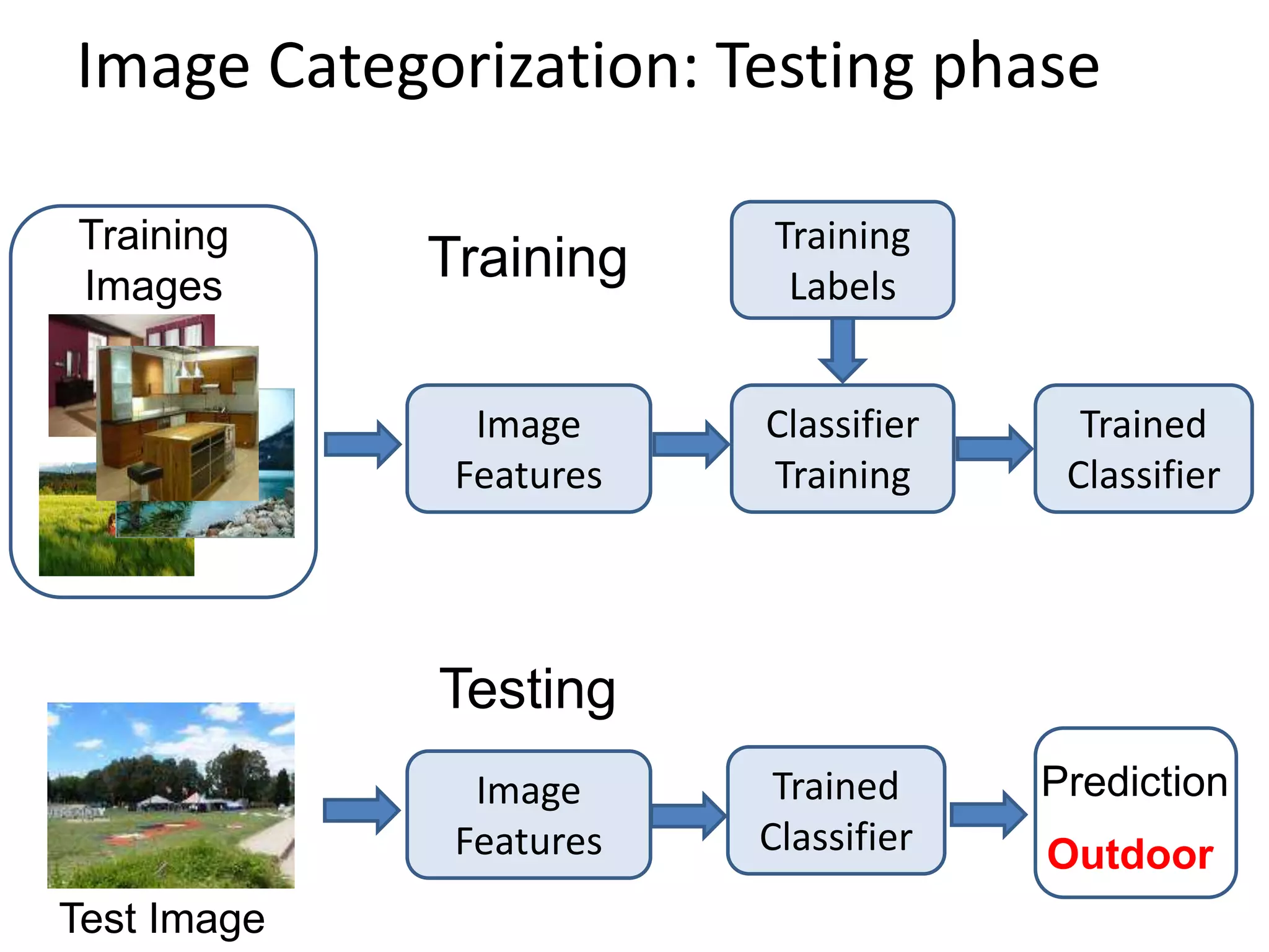
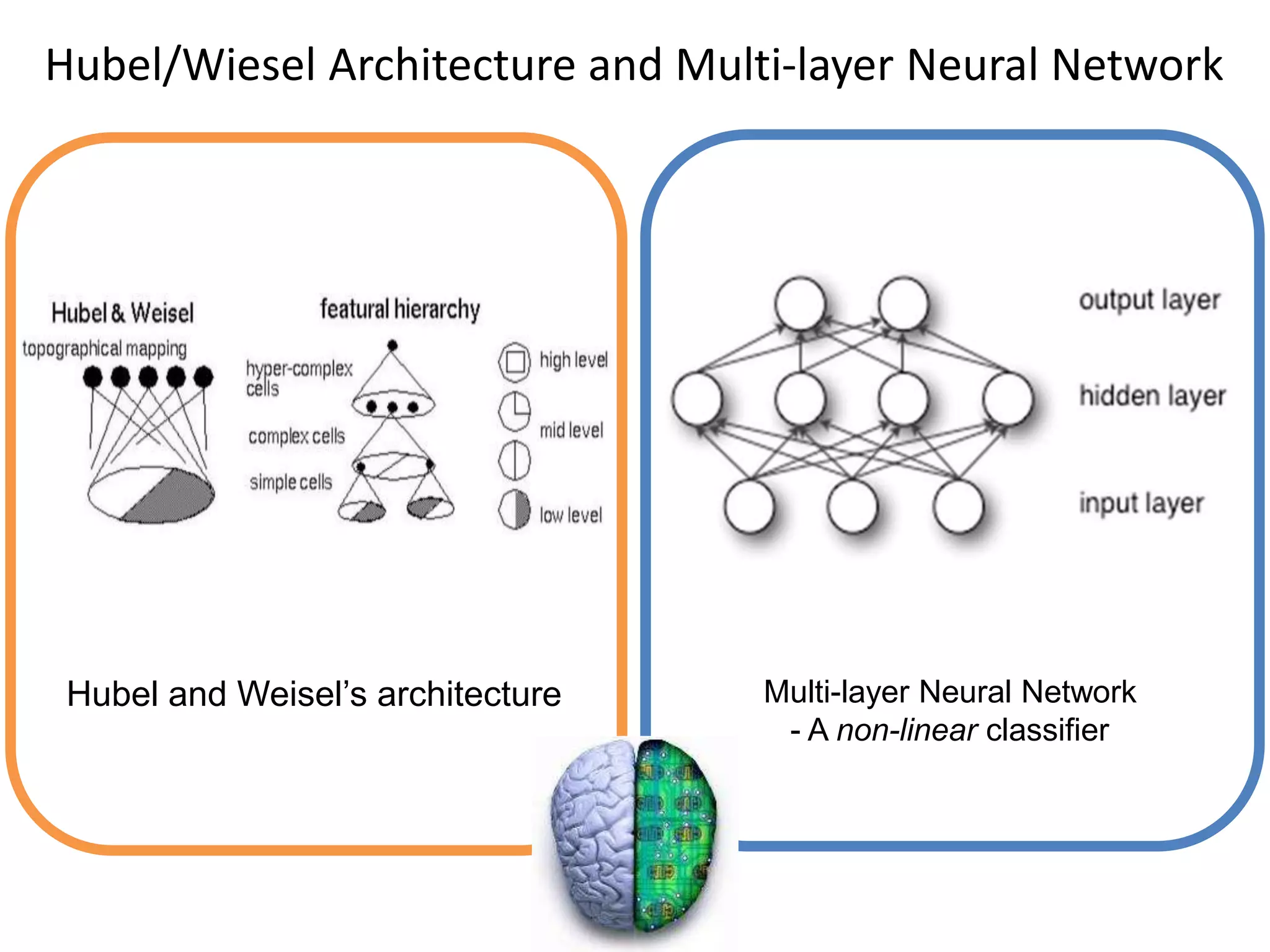
The document provides an overview of convolutional neural networks (CNNs) in computer vision, detailing their structure, training processes, and applications such as image classification and segmentation. It discusses the evolution of CNNs, techniques like backpropagation and transfer learning, and methods for understanding and visualizing CNNs. Additionally, it highlights important architectures, training strategies, and recent advancements in the field.


![[OSGeo-KR Tech Workshop] Deep Learning for Single Image Super-Resolution](https://cdn.slidesharecdn.com/ss_thumbnails/osgeo-krdeeplearningforsingleimagesuper-resolution-180223175347-thumbnail.jpg?width=640&height=640&fit=bounds)


![[Revised] Intro to CNN](https://cdn.slidesharecdn.com/ss_thumbnails/googletechsprinttalkcnnintro-200730141604-thumbnail.jpg?width=640&height=640&fit=bounds)


![ANPARA THERMAL POWER STATION[1] sangam.pdf](https://cdn.slidesharecdn.com/ss_thumbnails/anparathermalpowerstation1sangam-251121115219-9261cde4-thumbnail.jpg?width=640&height=640&fit=bounds)


