Downloaded 110 times
![Principles
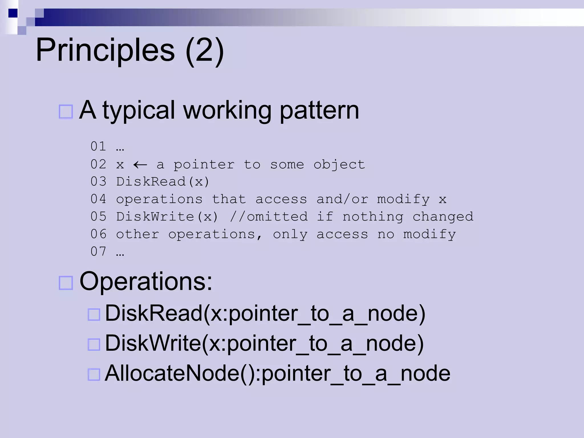
Pointers in data structures are no longer
addresses in main memory but
locations in files
If x is a pointer to an object
ifx is in main memory key[x] refers to it
otherwise DiskRead(x) reads the object
from disk into main memory (DiskWrite(x) –
writes it back to disk)](https://image.slidesharecdn.com/lec16-101217101514-phpapp01/75/Lec16-4-2048.jpg)
![B-tree Definitions
Node x has fields
n[x]: the number of keys of that the node
key1[x] … keyn[x][x]: the keys in ascending order
leaf[x]: true if leaf node, false if internal node
if internal node, then c1[x], …, cn[x]+1[x]: pointers to
children
Keys separate the ranges of keys in the sub-
trees. If ki is an arbitrary key in the subtree ci[x]
then ki keyi[x] ki+1](https://image.slidesharecdn.com/lec16-101217101514-phpapp01/75/Lec16-7-2048.jpg)
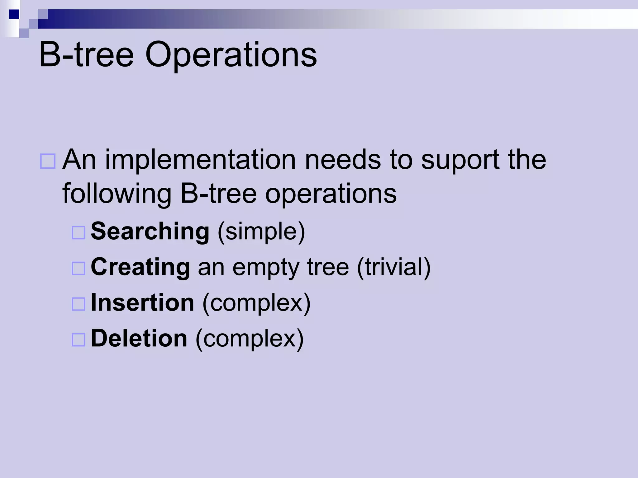
![Searching
Straightforward generalization of a binary
tree search
BTreeSearch(x,k)
01 i 1
02 while i n[x] and k > keyi[x]
03 i i+1
04 if i n[x] and k = keyi[x] then
05 return(x,i)
06 if leaf[x] then
08 return NIL
09 else DiskRead(ci[x])
10 return BTtreeSearch(ci[x],k)](https://image.slidesharecdn.com/lec16-101217101514-phpapp01/75/Lec16-11-2048.jpg)
![Creating an Empty Tree
Empty B-tree = create a root & write it to
disk!
BTreeCreate(T)
01 x AllocateNode();
02 leaf[x] TRUE;
03 n[x] 0;
04 DiskWrite(x);
05 root[T] x](https://image.slidesharecdn.com/lec16-101217101514-phpapp01/75/Lec16-12-2048.jpg)
![Splitting Nodes (2)
Result:
one key of x moves up to parent +
2 nodes with t-1 keys
x x
... N W ... ... N S W ...
y = ci[x]
y = ci[x] z = ci+1[x]
P Q R S T V W
P Q R T V W
T1 ... T8](https://image.slidesharecdn.com/lec16-101217101514-phpapp01/75/Lec16-14-2048.jpg)
![Splitting Nodes (2)
BTreeSplitChild(x,i,y)
z AllocateNode()
leaf[z] leaf[y] x: parent node
n[z] t-1 y: node to be split and child of x
for j 1 to t-1 i: index in x
keyj[z] keyj+t[y]
z: new node
if not leaf[y] then
for j 1 to t
cj[z] cj+t[y]
n[y] t-1 x
for j n[x]+1 downto i+1
cj+1[x] cj[x] ... N W ...
ci+1[x] z
for j n[x] downto i y = ci[x]
keyj+1[x] keyj[x]
keyi[x] keyt[y] P Q R S T V W
n[x] n[x]+1
DiskWrite(y)
DiskWrite(z) T1 ... T8
DiskWrite(x)](https://image.slidesharecdn.com/lec16-101217101514-phpapp01/75/Lec16-15-2048.jpg)
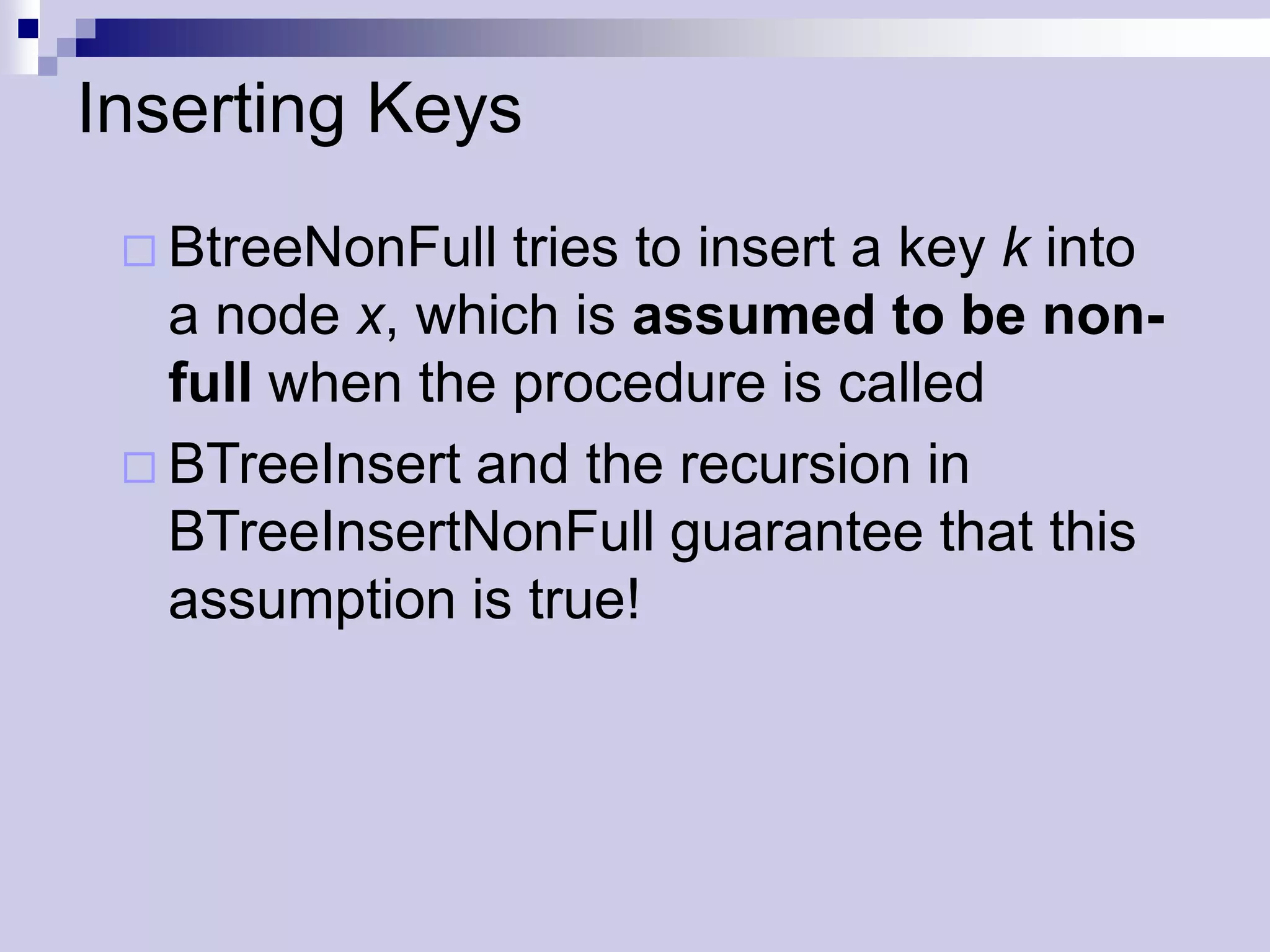
![Inserting Keys (2)
Special case: root is full (BtreeInsert)
BTreeInsert(T)
r root[T]
if n[r] = 2t – 1 then
s AllocateNode()
root[T] s
leaf[s] FALSE
n[s] 0
c1[s] r
BTreeSplitChild(s,1,r)
BTreeInsertNonFull(s,k)
else BTreeInsertNonFull(r,k)](https://image.slidesharecdn.com/lec16-101217101514-phpapp01/75/Lec16-18-2048.jpg)
![Splitting the Root
Splitting the root requires the creation of a
new root
root[T]
root[T] s
r
H
A D F H L N P
r
A D F L N P
T1 ... T8
The tree grows at the top instead of the
bottom](https://image.slidesharecdn.com/lec16-101217101514-phpapp01/75/Lec16-19-2048.jpg)
![Inserting Keys: Pseudo Code
BTreeInsertNonFull(x,k)
01 i n[x]
02 if leaf[x] then
03 while i 1 and k < keyi[x]
04 keyi+1[x] keyi[x]
05 i i - 1 leaf insertion
06 keyi+1[x] k
07 n[x] n[x] + 1
08 DiskWrite(x)
09 else while i 1 and k < keyi[x]
10 i i - 1
11 i i + 1 internal node:
12 DiskRead ci[x] traversing tree
13 if n[ci[x]] = 2t – 1 then
14 BTreeSplitChild(x,i,ci[x])
15 if k > keyi[x] then
16 i i + 1
17 BTreeInsertNonFull(ci[x],k)](https://image.slidesharecdn.com/lec16-101217101514-phpapp01/75/Lec16-21-2048.jpg)
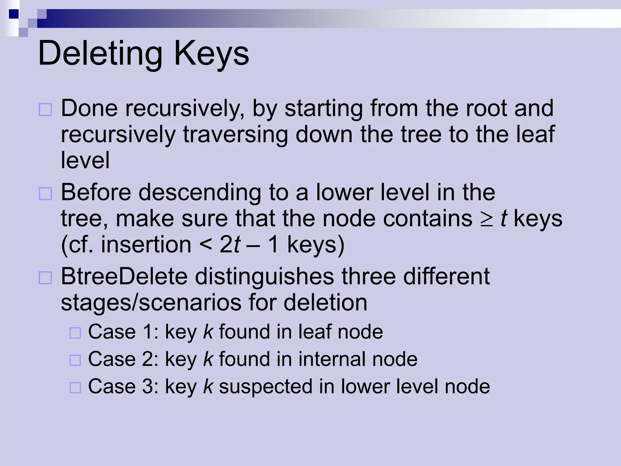
![Deleting Keys - Distribution
Descending down the tree: if k not found in
current node x, find the sub-tree ci[x] that has to
contain k.
If ci[x] has only t – 1 keys take action to ensure
that we descent to a node of size at least t.
We can encounter two cases.
If ci[x] has only t-1 keys, but a sibling with at least t
keys, give ci[x] an extra key by moving a key from x to
ci[x], moving a key from ci[x]’s immediate left and right
sibling up into x, and moving the appropriate child from
the sibling into ci[x] - distribution](https://image.slidesharecdn.com/lec16-101217101514-phpapp01/75/Lec16-29-2048.jpg)
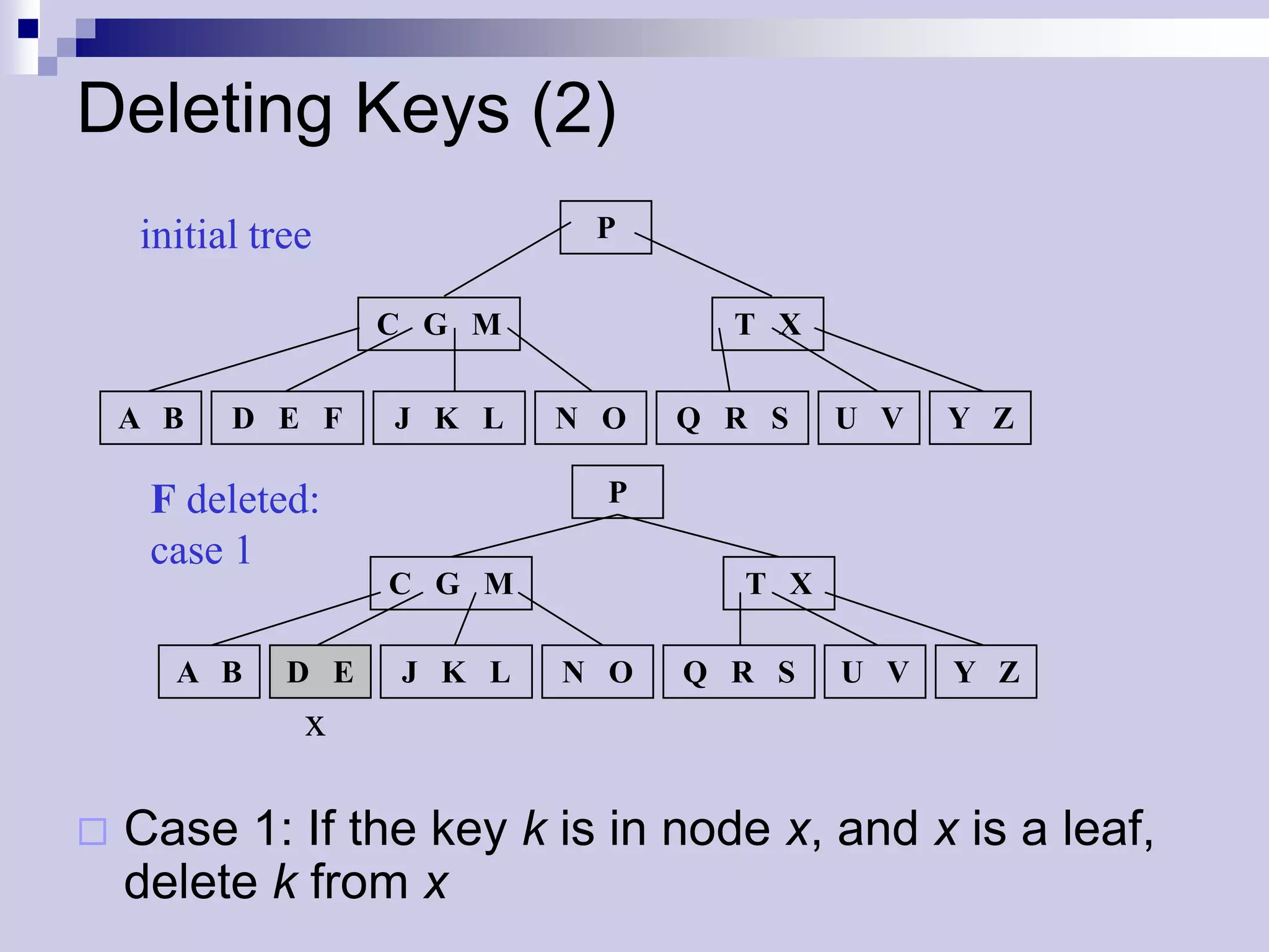
![Deleting Keys – Distribution(2)
x ... k ... x ... k’ ...
ci[x] ... k’ ci[x] ... k
A B A B
C L P T X
delete B
ci[x] A B E J K N O Q R S U V Y Z
sibling
B deleted: E L P T X
A C J K N O Q R S U V Y Z](https://image.slidesharecdn.com/lec16-101217101514-phpapp01/75/Lec16-30-2048.jpg)
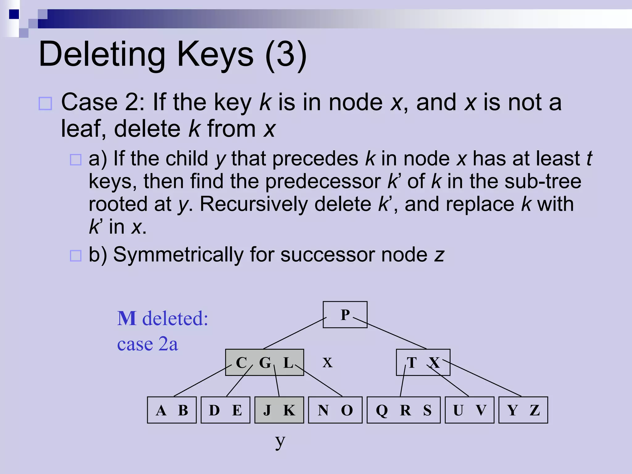
![Deleting Keys - Merging
If ci[x] and both of ci[x]’s siblings have t – 1
keys, merge ci with one sibling, which
involves moving a key from x down into
the new merged node to become the
median key for that node
x ... l’ k m’... x ... l’ m’ ...
ci[x] ... l m… ...l k m ...
A B A B](https://image.slidesharecdn.com/lec16-101217101514-phpapp01/75/Lec16-31-2048.jpg)
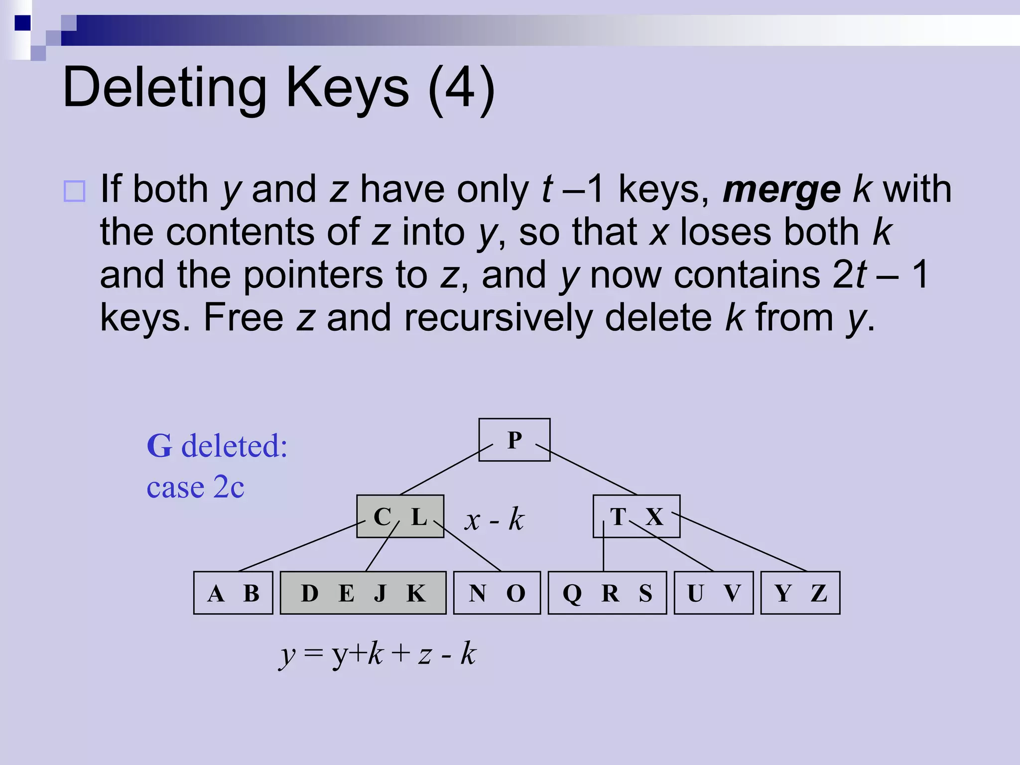
![Deleting Keys – Merging (2)
P
delete D ci[x] C L sibling T X
A B D E J K N O Q R S U V Y Z
D deleted:
C L P T X
A B E J K N O Q R S U V Y Z
tree shrinks in height](https://image.slidesharecdn.com/lec16-101217101514-phpapp01/75/Lec16-32-2048.jpg)


![Principles
Pointers in data structures are no longer
addresses in main memory but
locations in files
If x is a pointer to an object
ifx is in main memory key[x] refers to it
otherwise DiskRead(x) reads the object
from disk into main memory (DiskWrite(x) –
writes it back to disk)](https://crownmelresort.com/image.slidesharecdn.com/lec16-101217101514-phpapp01/75/Lec16-4-2048.jpg)


![B-tree Definitions
Node x has fields
n[x]: the number of keys of that the node
key1[x] … keyn[x][x]: the keys in ascending order
leaf[x]: true if leaf node, false if internal node
if internal node, then c1[x], …, cn[x]+1[x]: pointers to
children
Keys separate the ranges of keys in the sub-
trees. If ki is an arbitrary key in the subtree ci[x]
then ki keyi[x] ki+1](https://crownmelresort.com/image.slidesharecdn.com/lec16-101217101514-phpapp01/75/Lec16-7-2048.jpg)


![Searching
Straightforward generalization of a binary
tree search
BTreeSearch(x,k)
01 i 1
02 while i n[x] and k > keyi[x]
03 i i+1
04 if i n[x] and k = keyi[x] then
05 return(x,i)
06 if leaf[x] then
08 return NIL
09 else DiskRead(ci[x])
10 return BTtreeSearch(ci[x],k)](https://crownmelresort.com/image.slidesharecdn.com/lec16-101217101514-phpapp01/75/Lec16-11-2048.jpg)
![Creating an Empty Tree
Empty B-tree = create a root & write it to
disk!
BTreeCreate(T)
01 x AllocateNode();
02 leaf[x] TRUE;
03 n[x] 0;
04 DiskWrite(x);
05 root[T] x](https://crownmelresort.com/image.slidesharecdn.com/lec16-101217101514-phpapp01/75/Lec16-12-2048.jpg)

![Splitting Nodes (2)
Result:
one key of x moves up to parent +
2 nodes with t-1 keys
x x
... N W ... ... N S W ...
y = ci[x]
y = ci[x] z = ci+1[x]
P Q R S T V W
P Q R T V W
T1 ... T8](https://crownmelresort.com/image.slidesharecdn.com/lec16-101217101514-phpapp01/75/Lec16-14-2048.jpg)
![Splitting Nodes (2)
BTreeSplitChild(x,i,y)
z AllocateNode()
leaf[z] leaf[y] x: parent node
n[z] t-1 y: node to be split and child of x
for j 1 to t-1 i: index in x
keyj[z] keyj+t[y]
z: new node
if not leaf[y] then
for j 1 to t
cj[z] cj+t[y]
n[y] t-1 x
for j n[x]+1 downto i+1
cj+1[x] cj[x] ... N W ...
ci+1[x] z
for j n[x] downto i y = ci[x]
keyj+1[x] keyj[x]
keyi[x] keyt[y] P Q R S T V W
n[x] n[x]+1
DiskWrite(y)
DiskWrite(z) T1 ... T8
DiskWrite(x)](https://crownmelresort.com/image.slidesharecdn.com/lec16-101217101514-phpapp01/75/Lec16-15-2048.jpg)


![Inserting Keys (2)
Special case: root is full (BtreeInsert)
BTreeInsert(T)
r root[T]
if n[r] = 2t – 1 then
s AllocateNode()
root[T] s
leaf[s] FALSE
n[s] 0
c1[s] r
BTreeSplitChild(s,1,r)
BTreeInsertNonFull(s,k)
else BTreeInsertNonFull(r,k)](https://crownmelresort.com/image.slidesharecdn.com/lec16-101217101514-phpapp01/75/Lec16-18-2048.jpg)
![Splitting the Root
Splitting the root requires the creation of a
new root
root[T]
root[T] s
r
H
A D F H L N P
r
A D F L N P
T1 ... T8
The tree grows at the top instead of the
bottom](https://crownmelresort.com/image.slidesharecdn.com/lec16-101217101514-phpapp01/75/Lec16-19-2048.jpg)

![Inserting Keys: Pseudo Code
BTreeInsertNonFull(x,k)
01 i n[x]
02 if leaf[x] then
03 while i 1 and k < keyi[x]
04 keyi+1[x] keyi[x]
05 i i - 1 leaf insertion
06 keyi+1[x] k
07 n[x] n[x] + 1
08 DiskWrite(x)
09 else while i 1 and k < keyi[x]
10 i i - 1
11 i i + 1 internal node:
12 DiskRead ci[x] traversing tree
13 if n[ci[x]] = 2t – 1 then
14 BTreeSplitChild(x,i,ci[x])
15 if k > keyi[x] then
16 i i + 1
17 BTreeInsertNonFull(ci[x],k)](https://crownmelresort.com/image.slidesharecdn.com/lec16-101217101514-phpapp01/75/Lec16-21-2048.jpg)


![Deleting Keys - Distribution
Descending down the tree: if k not found in
current node x, find the sub-tree ci[x] that has to
contain k.
If ci[x] has only t – 1 keys take action to ensure
that we descent to a node of size at least t.
We can encounter two cases.
If ci[x] has only t-1 keys, but a sibling with at least t
keys, give ci[x] an extra key by moving a key from x to
ci[x], moving a key from ci[x]’s immediate left and right
sibling up into x, and moving the appropriate child from
the sibling into ci[x] - distribution](https://crownmelresort.com/image.slidesharecdn.com/lec16-101217101514-phpapp01/75/Lec16-29-2048.jpg)
![Deleting Keys – Distribution(2)
x ... k ... x ... k’ ...
ci[x] ... k’ ci[x] ... k
A B A B
C L P T X
delete B
ci[x] A B E J K N O Q R S U V Y Z
sibling
B deleted: E L P T X
A C J K N O Q R S U V Y Z](https://crownmelresort.com/image.slidesharecdn.com/lec16-101217101514-phpapp01/75/Lec16-30-2048.jpg)
![Deleting Keys - Merging
If ci[x] and both of ci[x]’s siblings have t – 1
keys, merge ci with one sibling, which
involves moving a key from x down into
the new merged node to become the
median key for that node
x ... l’ k m’... x ... l’ m’ ...
ci[x] ... l m… ...l k m ...
A B A B](https://crownmelresort.com/image.slidesharecdn.com/lec16-101217101514-phpapp01/75/Lec16-31-2048.jpg)
![Deleting Keys – Merging (2)
P
delete D ci[x] C L sibling T X
A B D E J K N O Q R S U V Y Z
D deleted:
C L P T X
A B E J K N O Q R S U V Y Z
tree shrinks in height](https://crownmelresort.com/image.slidesharecdn.com/lec16-101217101514-phpapp01/75/Lec16-32-2048.jpg)


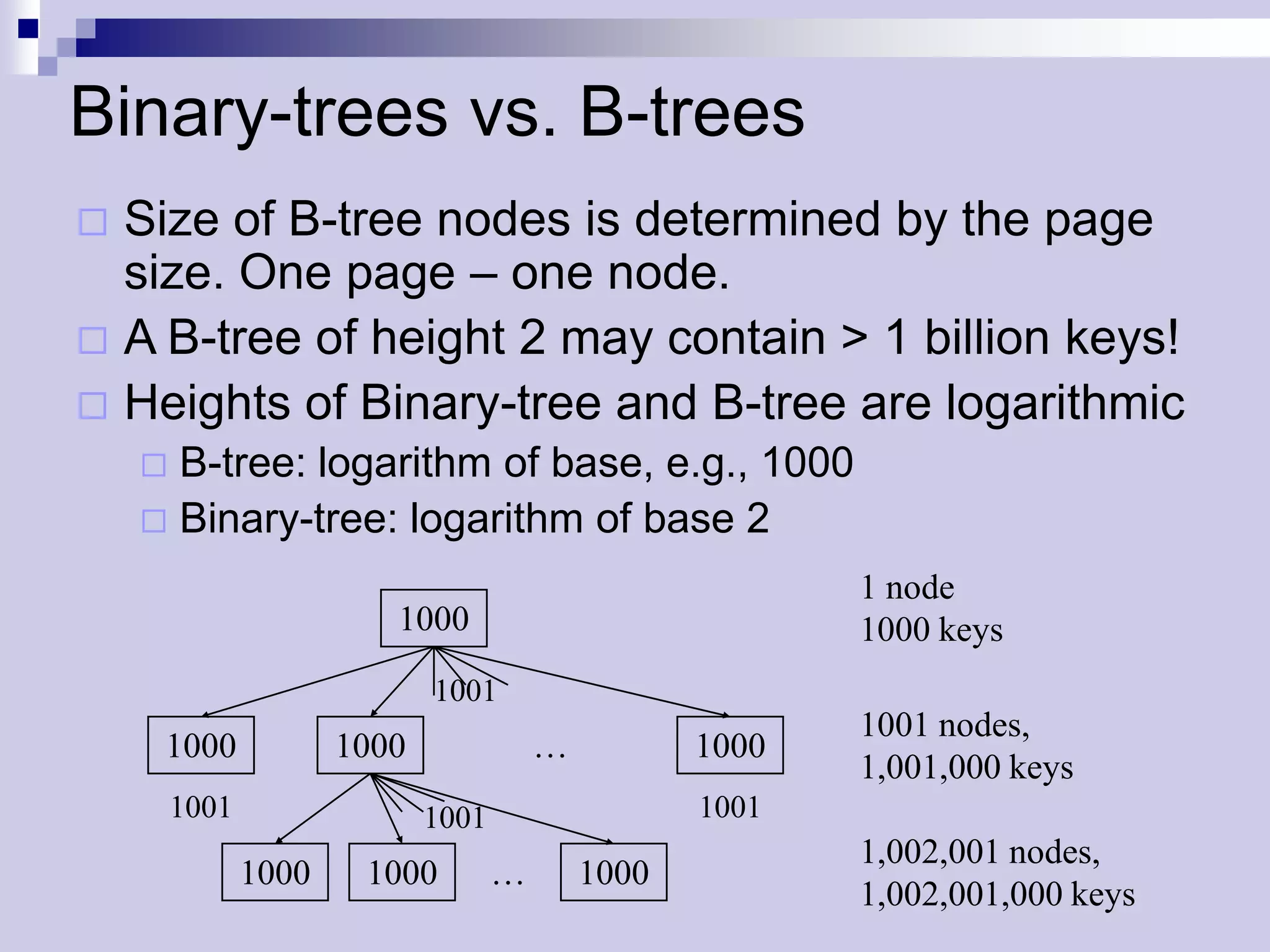
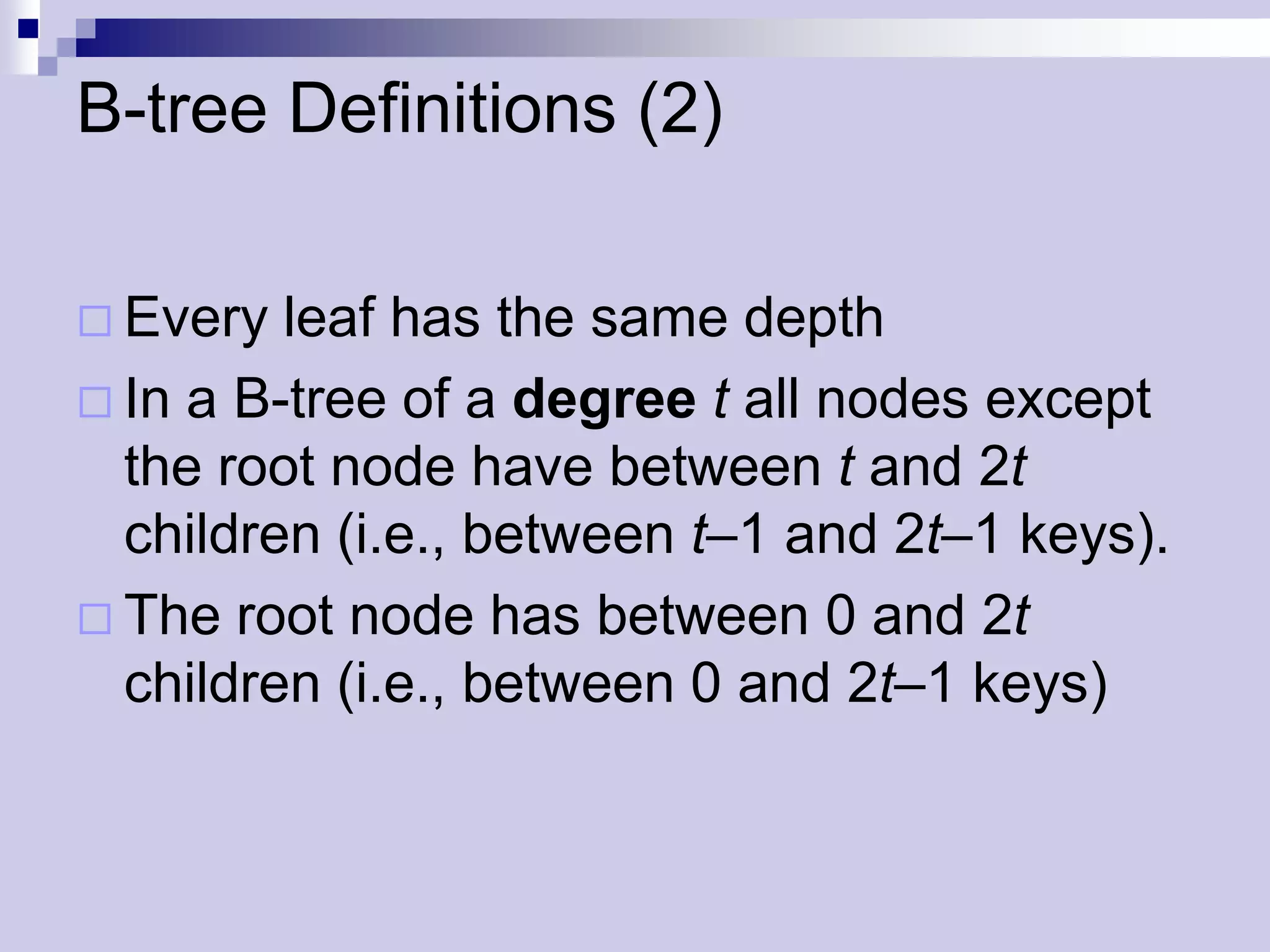
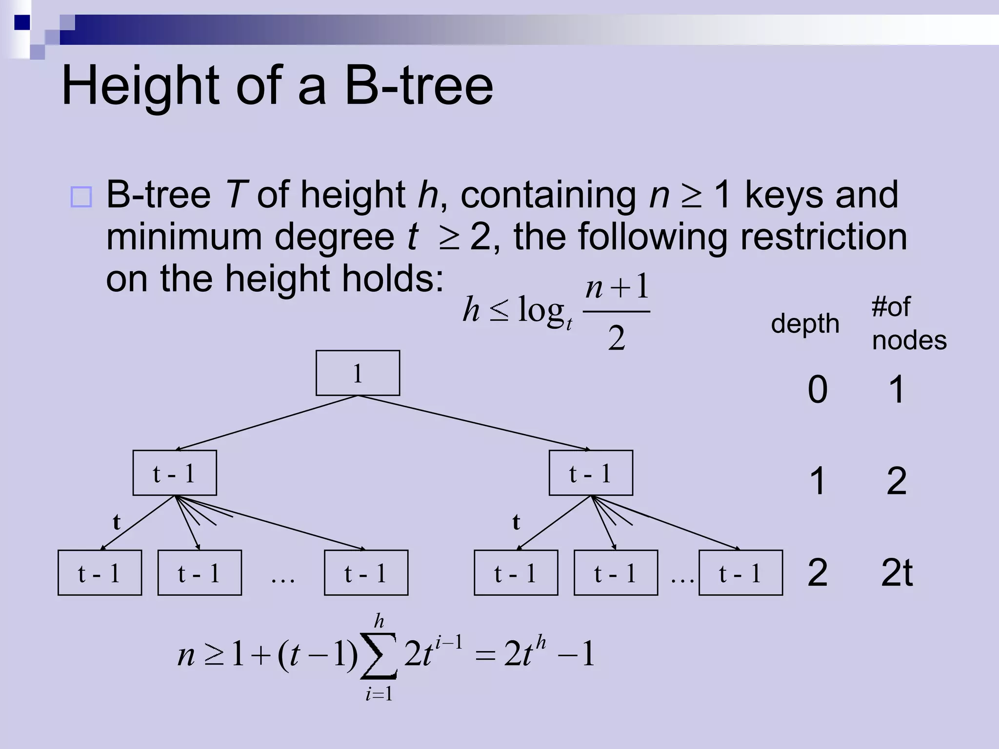
Disk-based data structures are needed to store large datasets that exceed main memory capacity. Hard disks allow large storage but have slow random access. B-trees address this by storing data in pages that can be read sequentially, keeping the tree shallow. Keys in B-tree nodes separate the ranges of keys in subtrees, and nodes have between t-1 and 2t-1 keys. Operations on B-trees like search, insert, and delete involve reading and writing nodes to disk and splitting or merging nodes as needed to maintain the B-tree properties.


![Presentation on b trees [autosaved]](https://cdn.slidesharecdn.com/ss_thumbnails/presentationonbtreesautosaved-210209155822-thumbnail.jpg?width=640&height=640&fit=bounds)