Downloaded 27 times

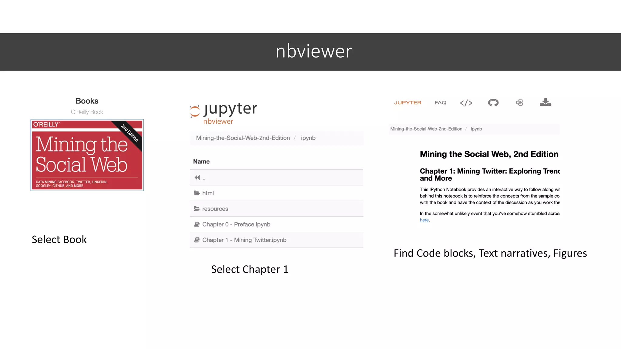


![Data Description – Categorical Data
32
value_counts() Returns counts for categorical values
Something is wrong
datasetname[‘columnname’].value_counts()
count()
Observations](https://image.slidesharecdn.com/jupyter-machine-learning-crash-cewit-2020-200308051902/75/Jupyter-machine-learning-crash-course-32-2048.jpg)
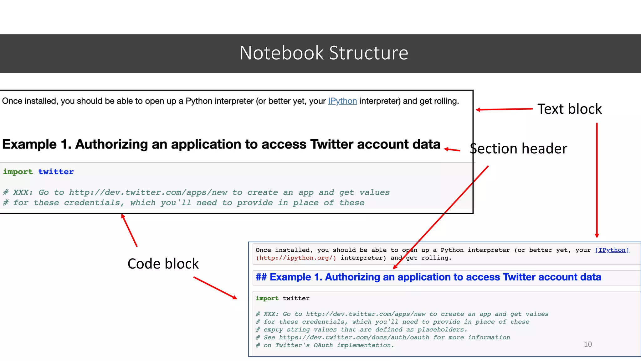
![Data Cleaning
replace()
33
replace by Iris-versicolor
replace by Iris-setosa
datasetname.replace(expression, substitution)
datasetname[‘column’].replace(expression, substitution)
Why CLASS has quotes?](https://image.slidesharecdn.com/jupyter-machine-learning-crash-cewit-2020-200308051902/75/Jupyter-machine-learning-crash-course-33-2048.jpg)
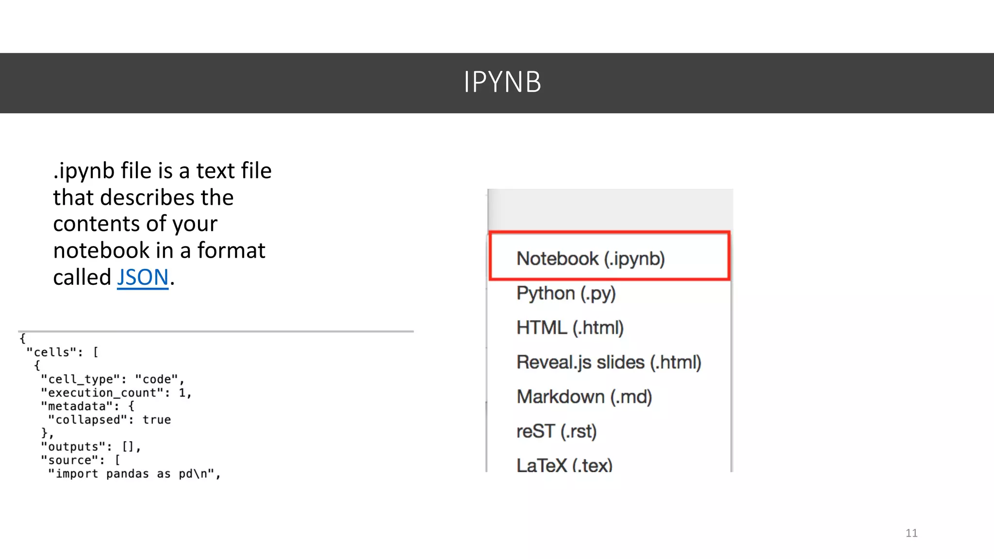
![Replacing NA by MEAN
36
1. Calculate MEAN for petal_width_cm
2. Replace missing values by MEAN
np.mean() Do you
remember what
NP is?
np.mean(datasetname[‘columnname’])
fillna()
datasetname[‘columnname’].fillna(value)
Create a new dataset (copy of iris)
Replace values by mean
inplace = changes will modify the current dataset](https://image.slidesharecdn.com/jupyter-machine-learning-crash-cewit-2020-200308051902/75/Jupyter-machine-learning-crash-course-36-2048.jpg)
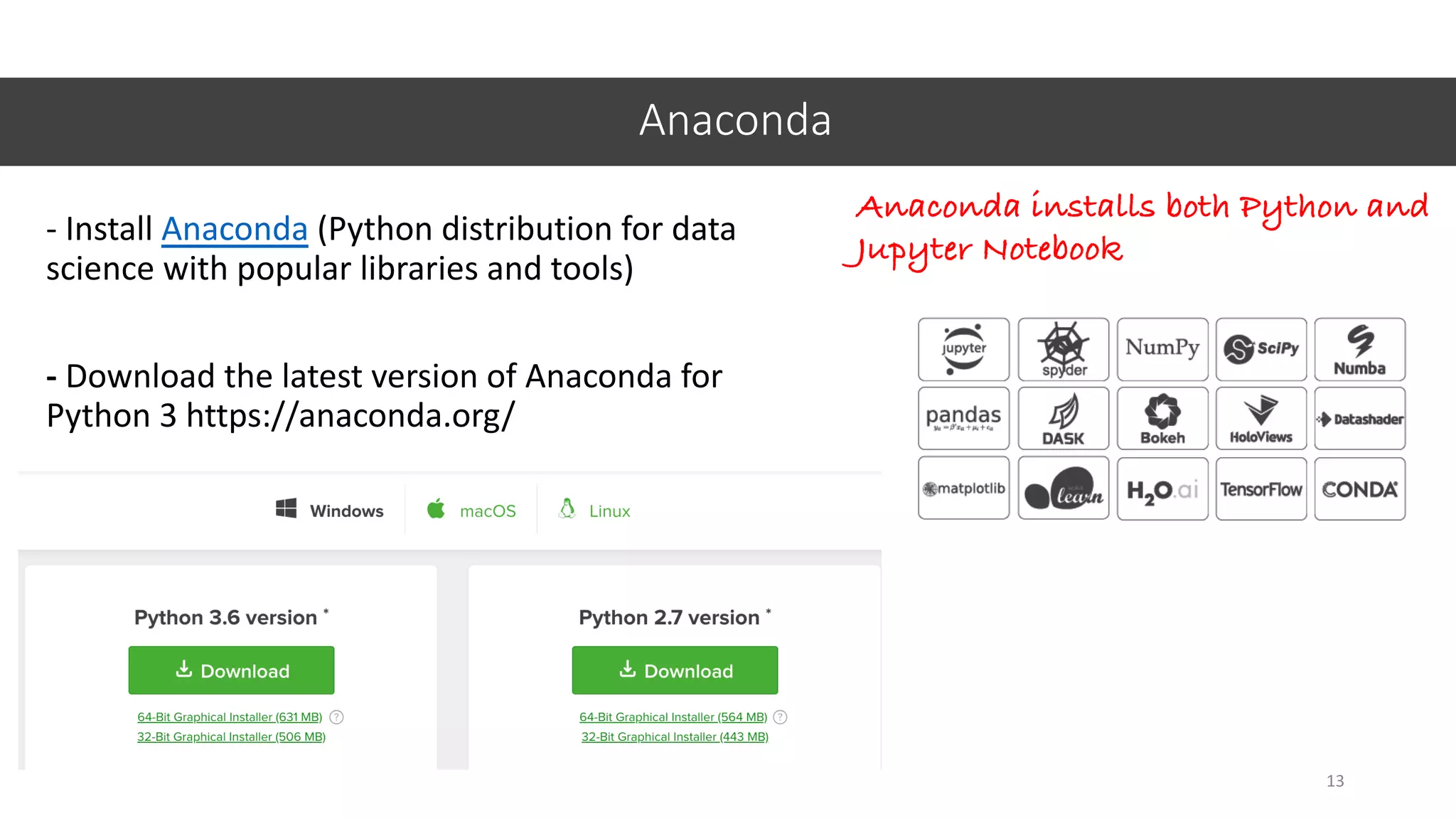
![Histograms
40
datasetname[‘columnname’].hist()hist()
Something is wrong!!](https://image.slidesharecdn.com/jupyter-machine-learning-crash-cewit-2020-200308051902/75/Jupyter-machine-learning-crash-course-40-2048.jpg)
![Selecting Outlier
42
(Condition 1) & (Condition 2)
IRIS-VERSICOLORand
iris_drop[‘sepal_length_cm’ <1] iris[‘class’ ==’Iris-versicolor’]&iris_drop](https://image.slidesharecdn.com/jupyter-machine-learning-crash-cewit-2020-200308051902/75/Jupyter-machine-learning-crash-course-42-2048.jpg)


![Data Description – Categorical Data
32
value_counts() Returns counts for categorical values
Something is wrong
datasetname[‘columnname’].value_counts()
count()
Observations](https://crownmelresort.com/image.slidesharecdn.com/jupyter-machine-learning-crash-cewit-2020-200308051902/75/Jupyter-machine-learning-crash-course-32-2048.jpg)
![Data Cleaning
replace()
33
replace by Iris-versicolor
replace by Iris-setosa
datasetname.replace(expression, substitution)
datasetname[‘column’].replace(expression, substitution)
Why CLASS has quotes?](https://crownmelresort.com/image.slidesharecdn.com/jupyter-machine-learning-crash-cewit-2020-200308051902/75/Jupyter-machine-learning-crash-course-33-2048.jpg)


![Replacing NA by MEAN
36
1. Calculate MEAN for petal_width_cm
2. Replace missing values by MEAN
np.mean() Do you
remember what
NP is?
np.mean(datasetname[‘columnname’])
fillna()
datasetname[‘columnname’].fillna(value)
Create a new dataset (copy of iris)
Replace values by mean
inplace = changes will modify the current dataset](https://crownmelresort.com/image.slidesharecdn.com/jupyter-machine-learning-crash-cewit-2020-200308051902/75/Jupyter-machine-learning-crash-course-36-2048.jpg)


![Histograms
40
datasetname[‘columnname’].hist()hist()
Something is wrong!!](https://crownmelresort.com/image.slidesharecdn.com/jupyter-machine-learning-crash-cewit-2020-200308051902/75/Jupyter-machine-learning-crash-course-40-2048.jpg)

![Selecting Outlier
42
(Condition 1) & (Condition 2)
IRIS-VERSICOLORand
iris_drop[‘sepal_length_cm’ <1] iris[‘class’ ==’Iris-versicolor’]&iris_drop](https://crownmelresort.com/image.slidesharecdn.com/jupyter-machine-learning-crash-cewit-2020-200308051902/75/Jupyter-machine-learning-crash-course-42-2048.jpg)


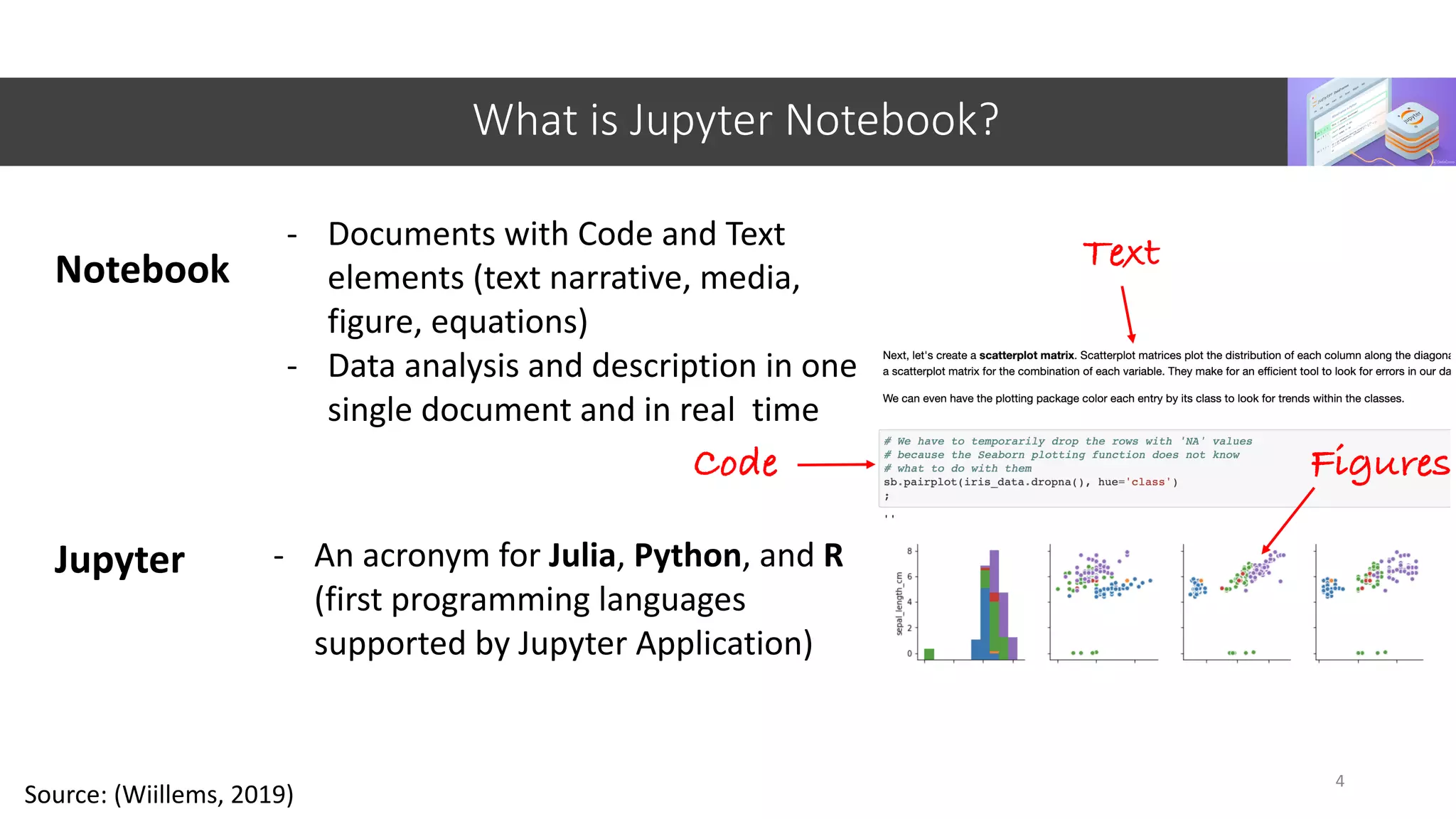
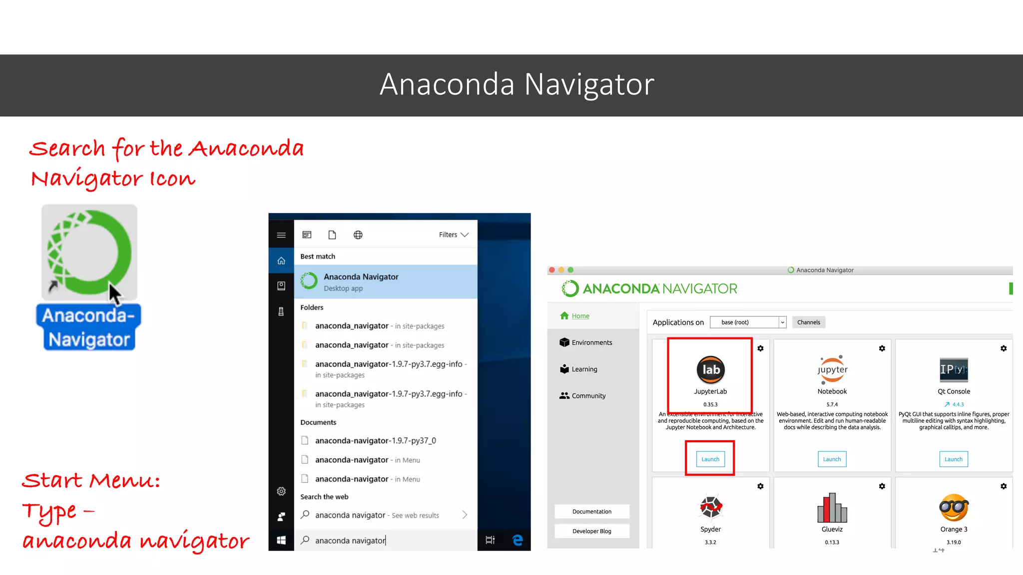
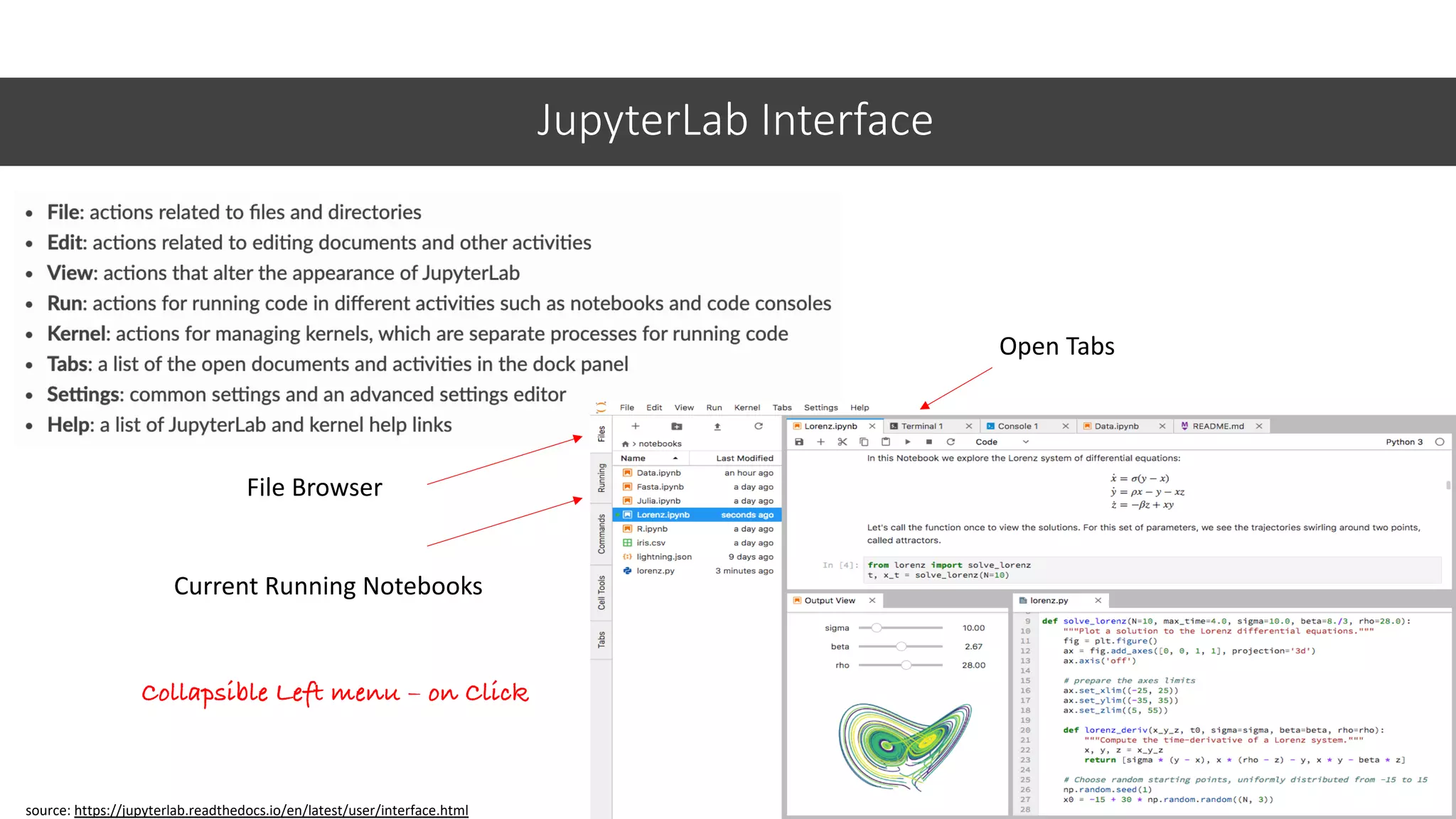
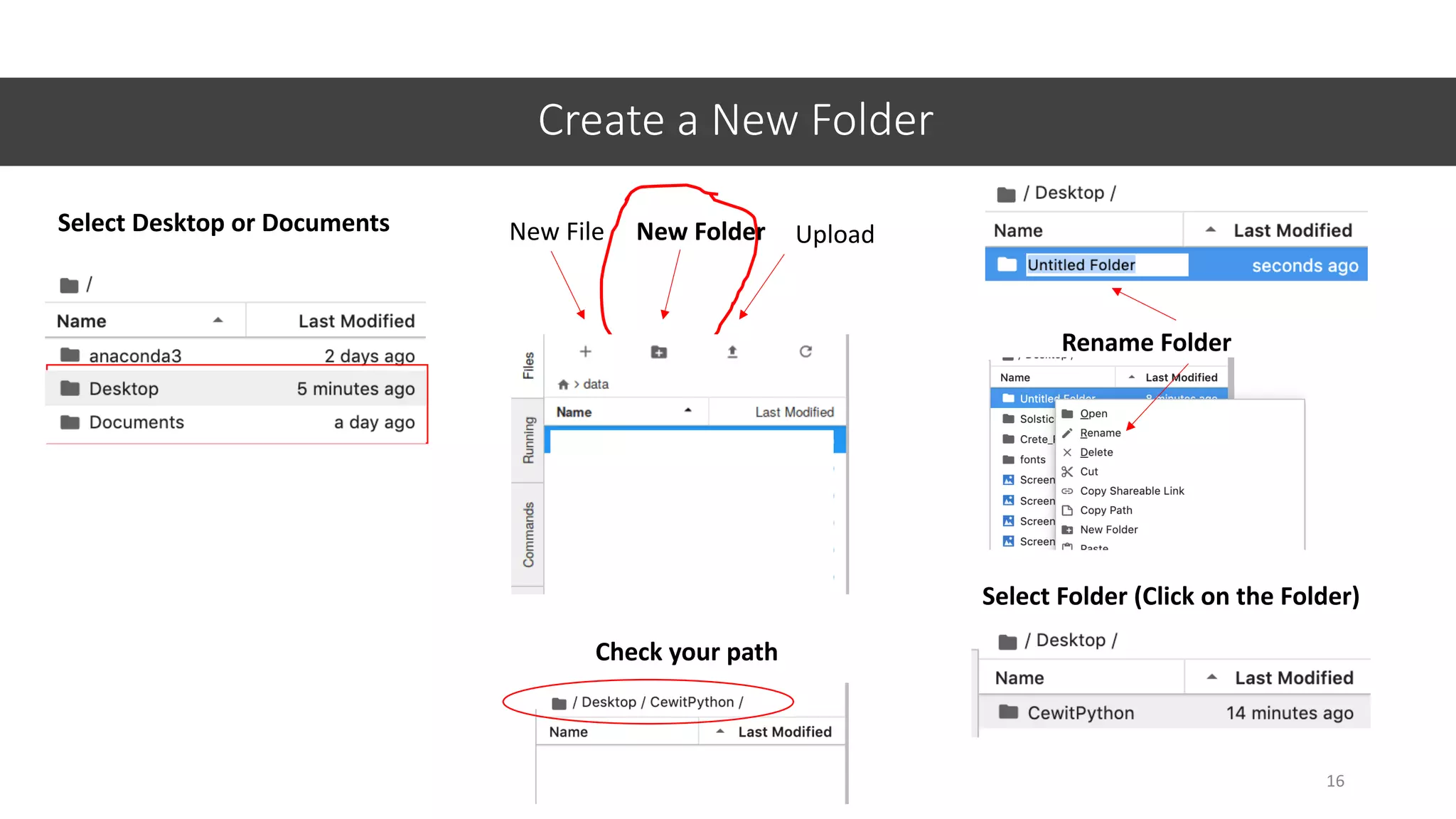
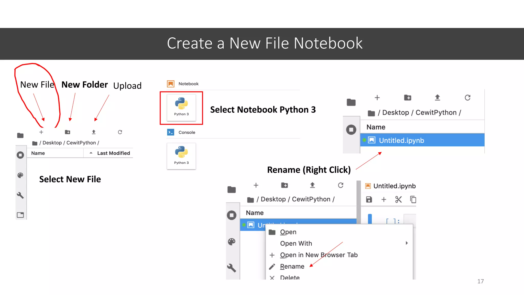
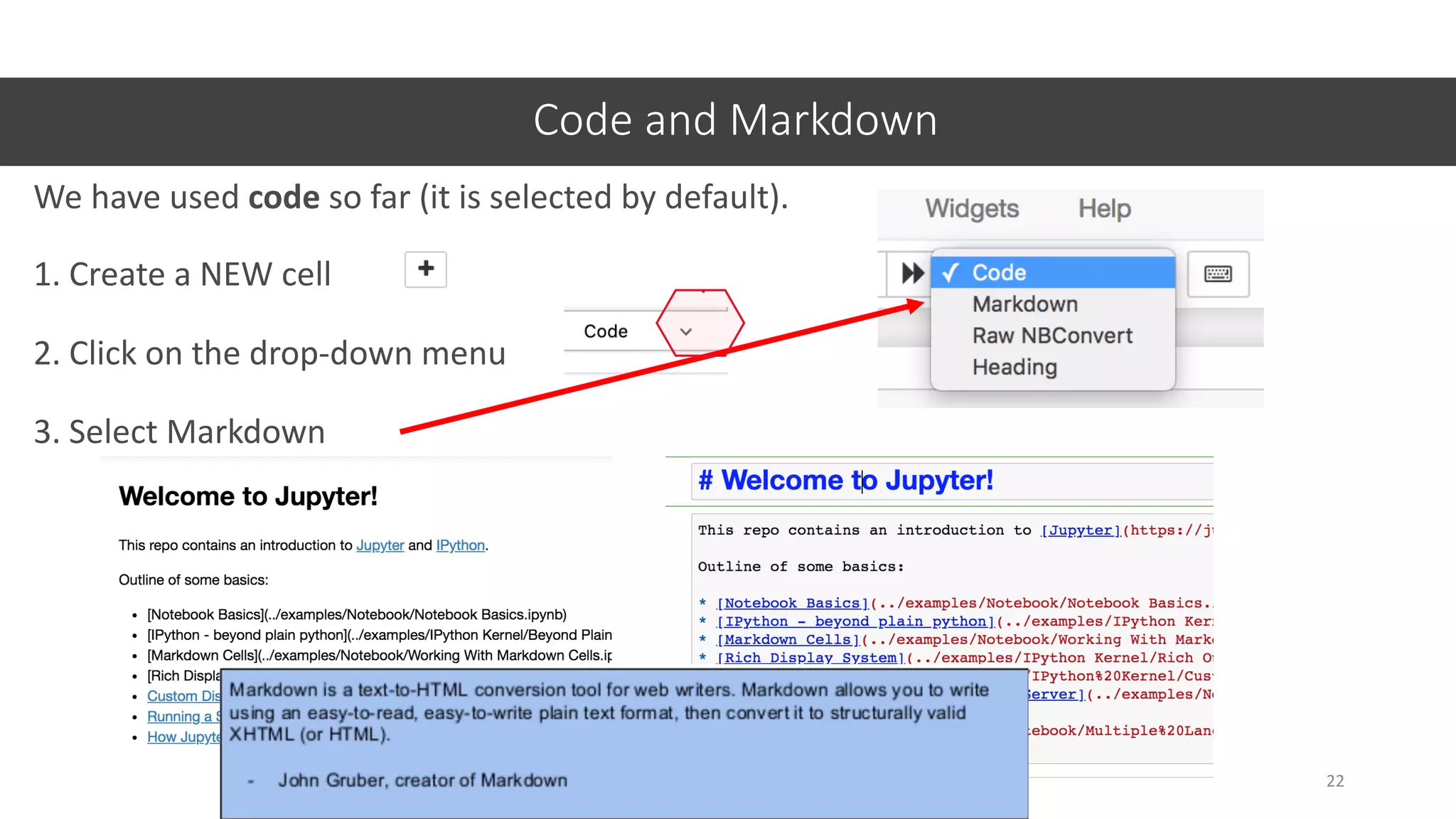
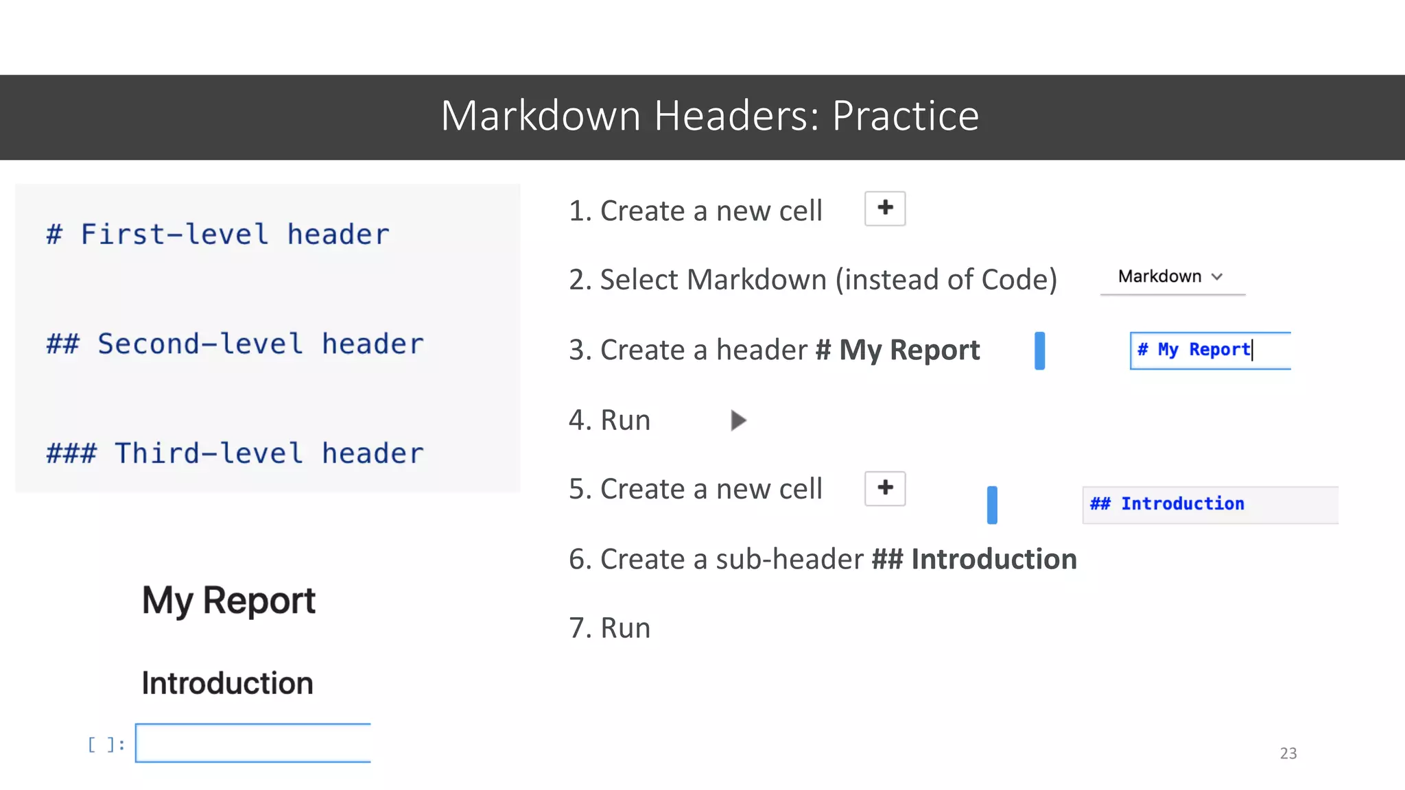
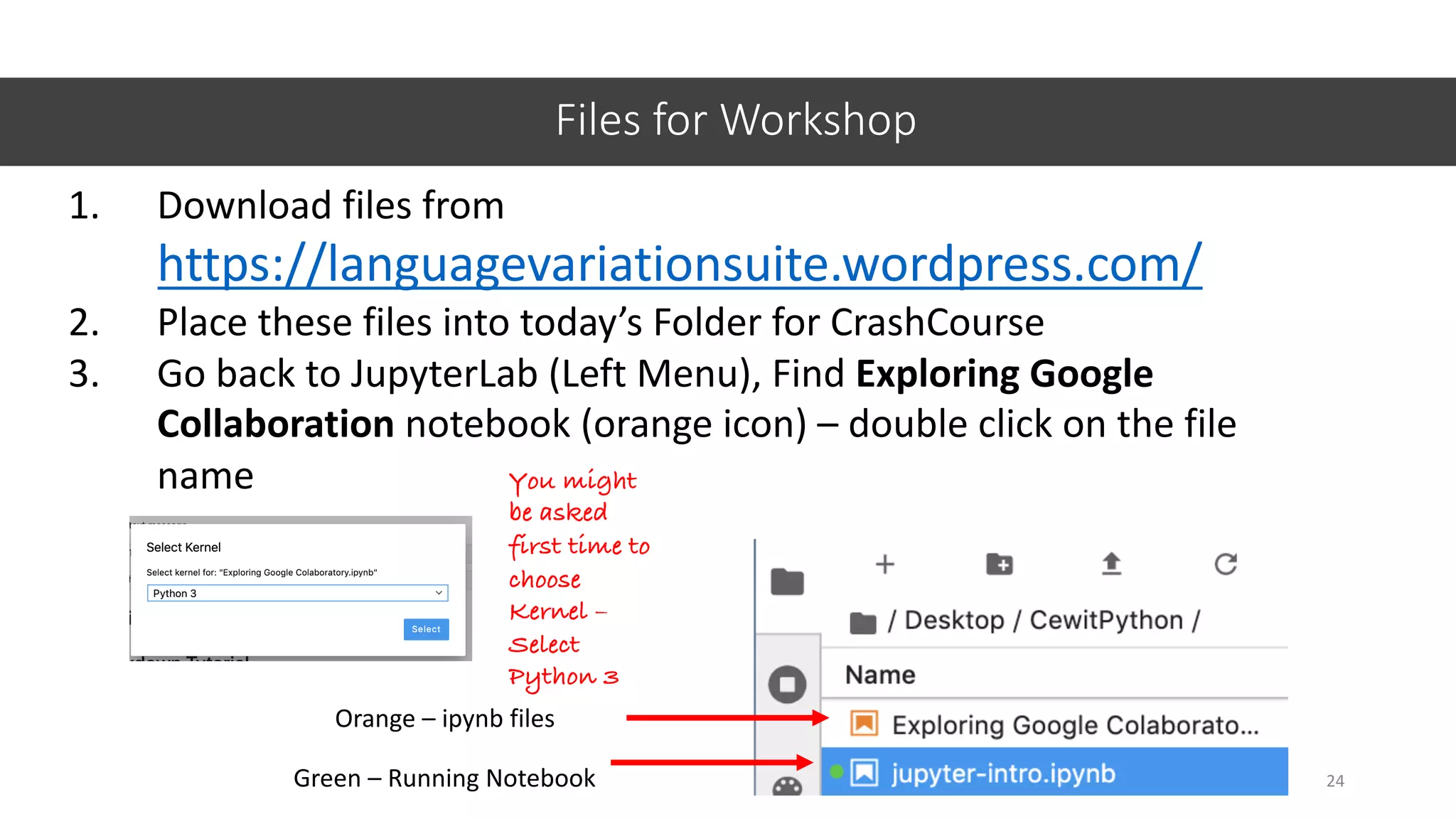
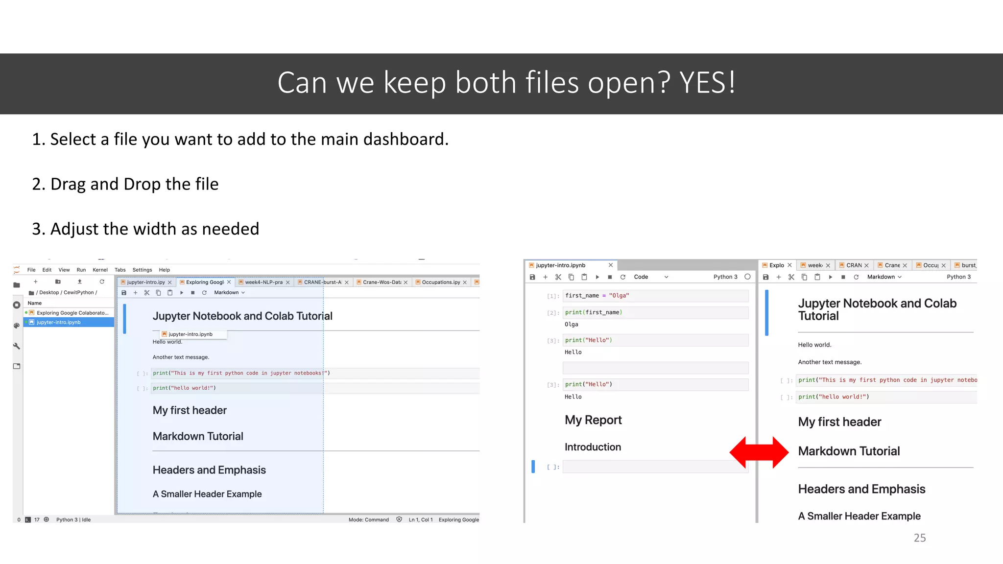
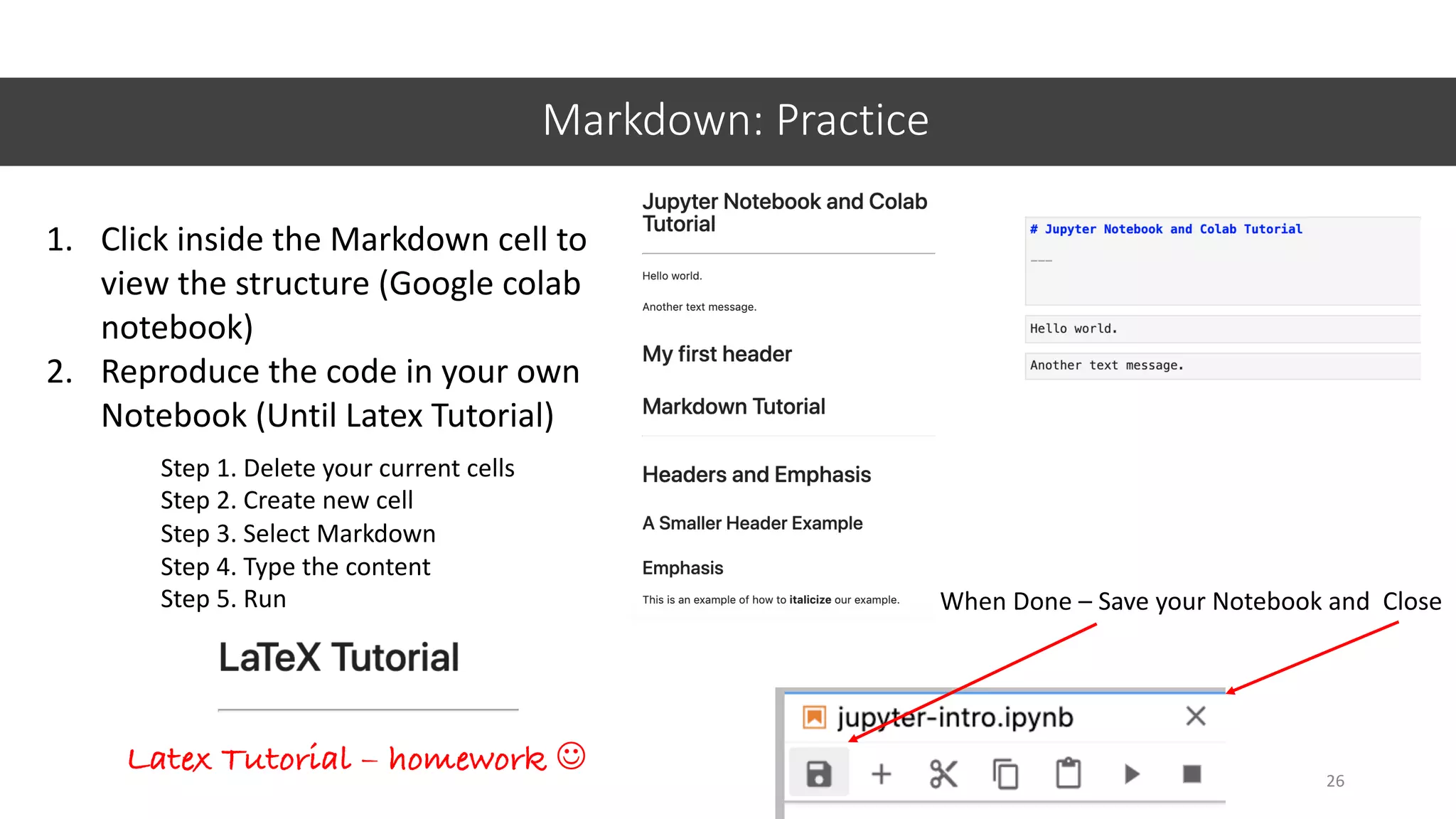
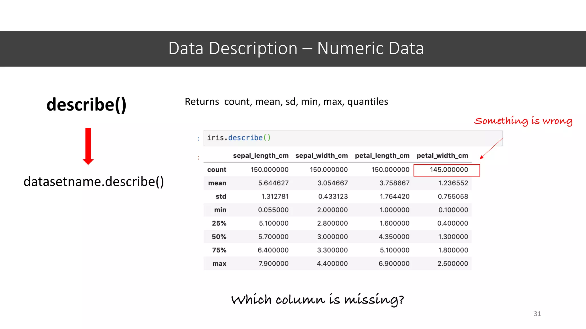
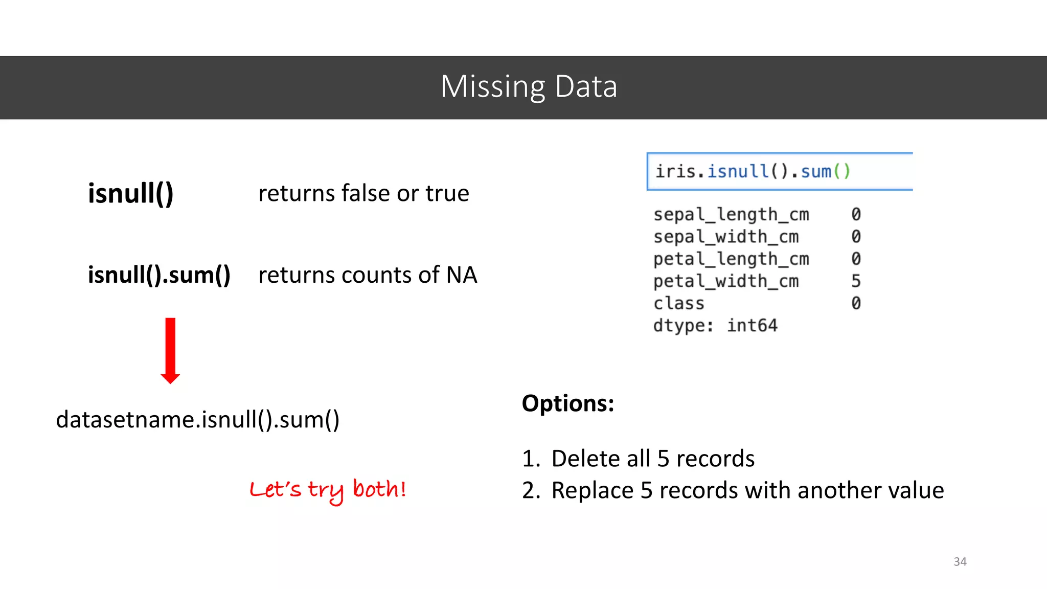
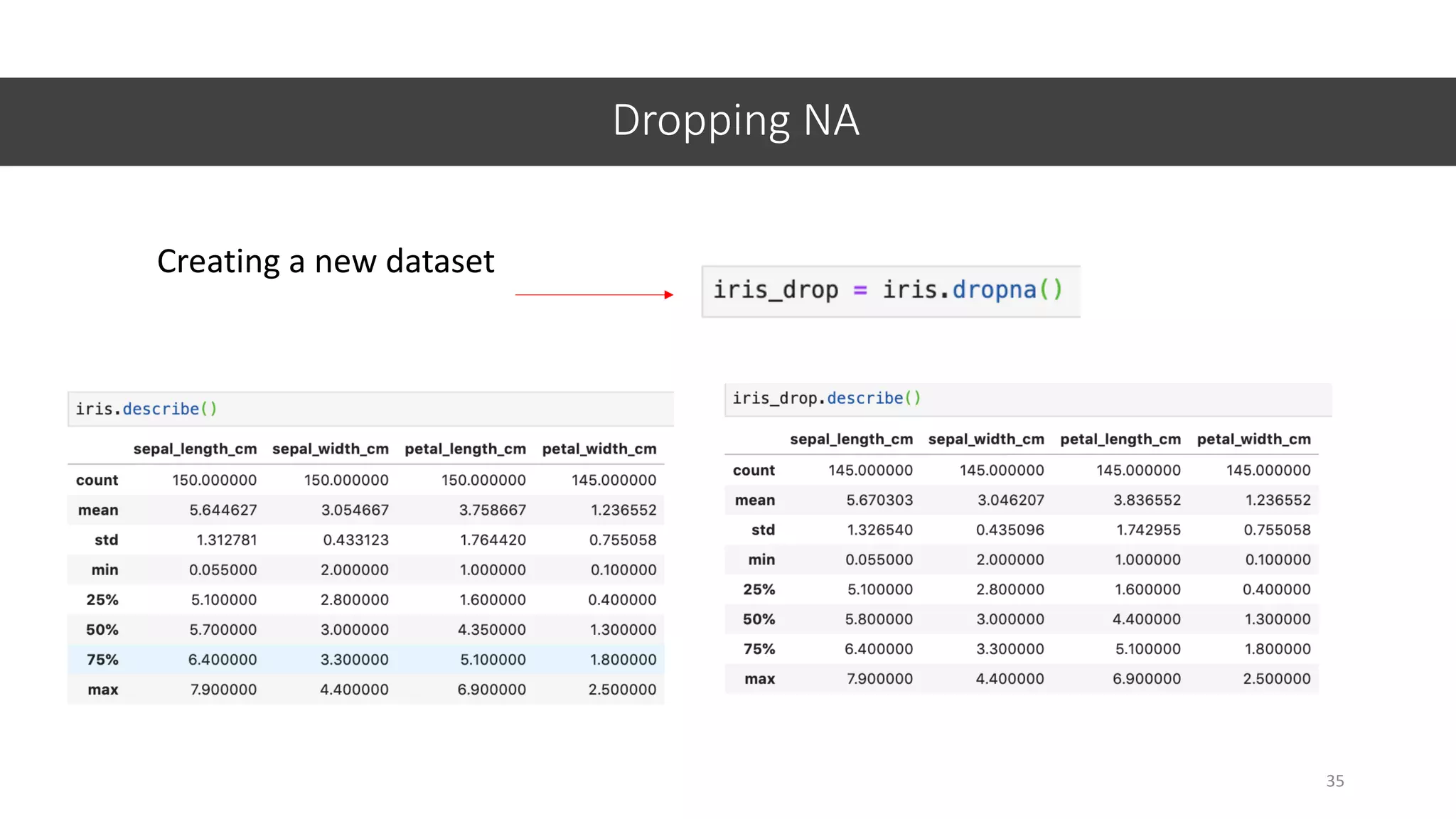
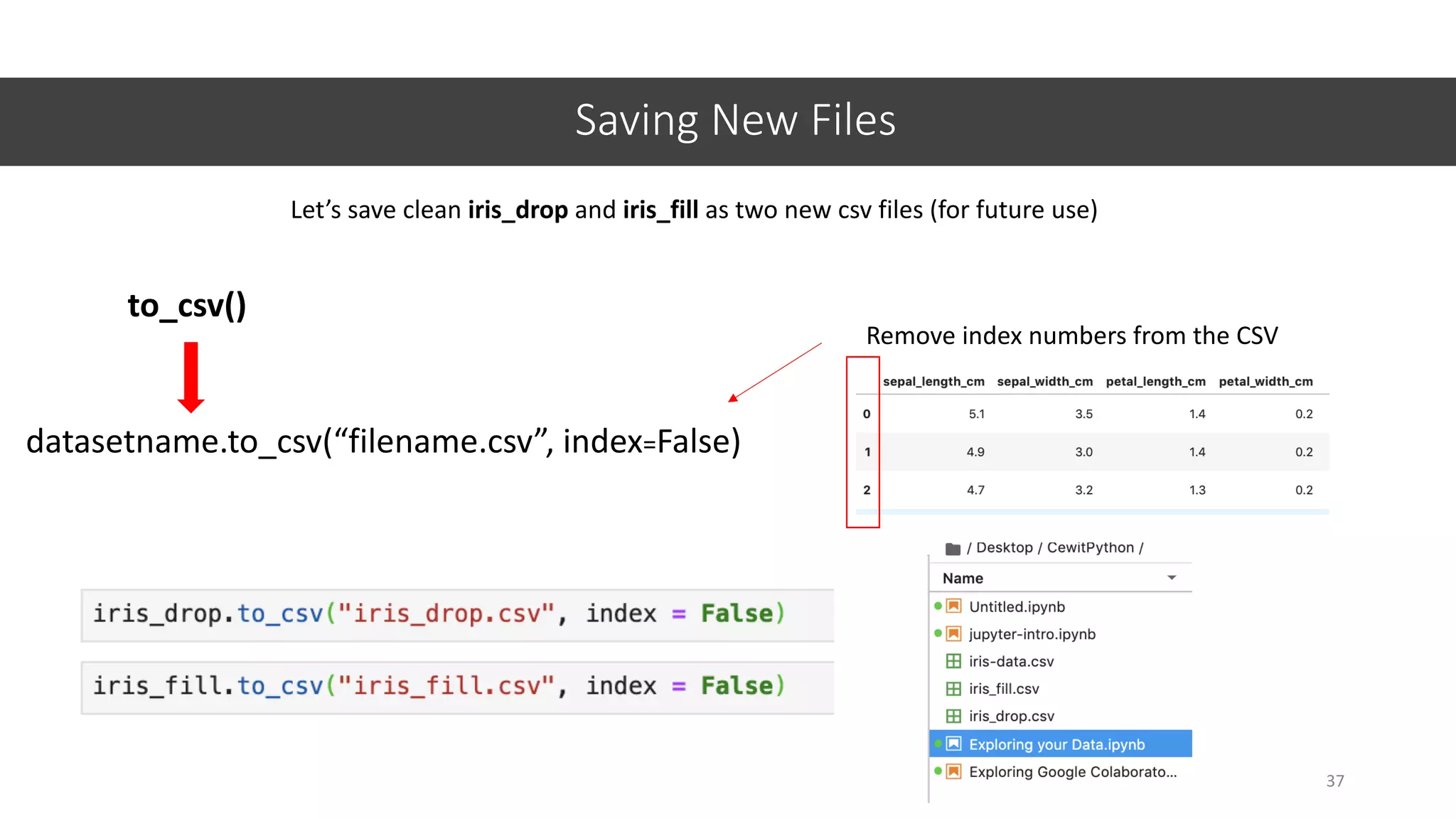
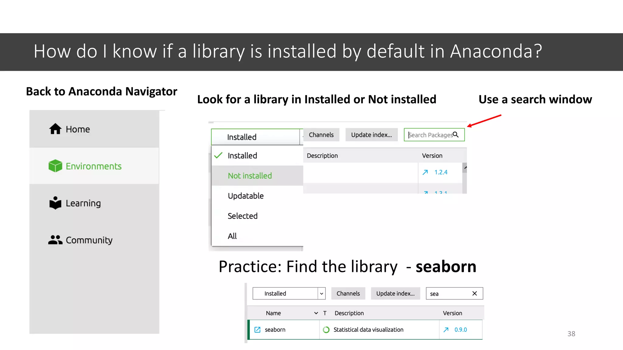
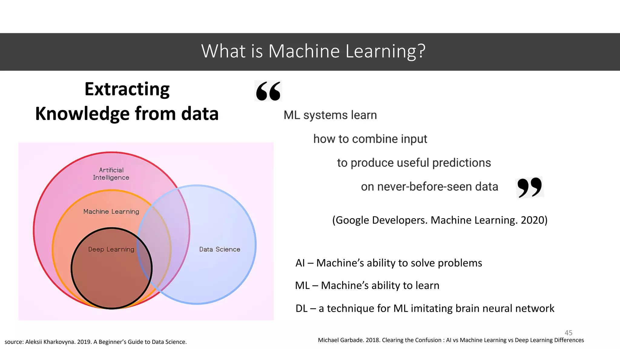
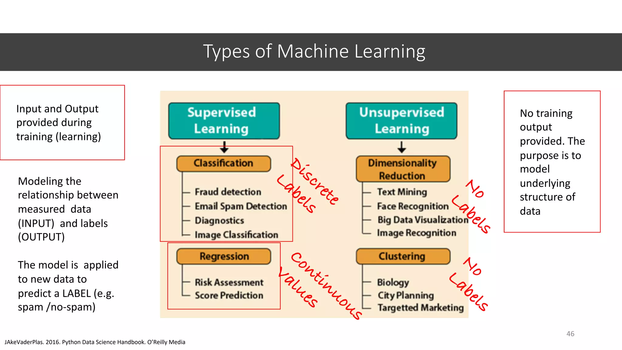
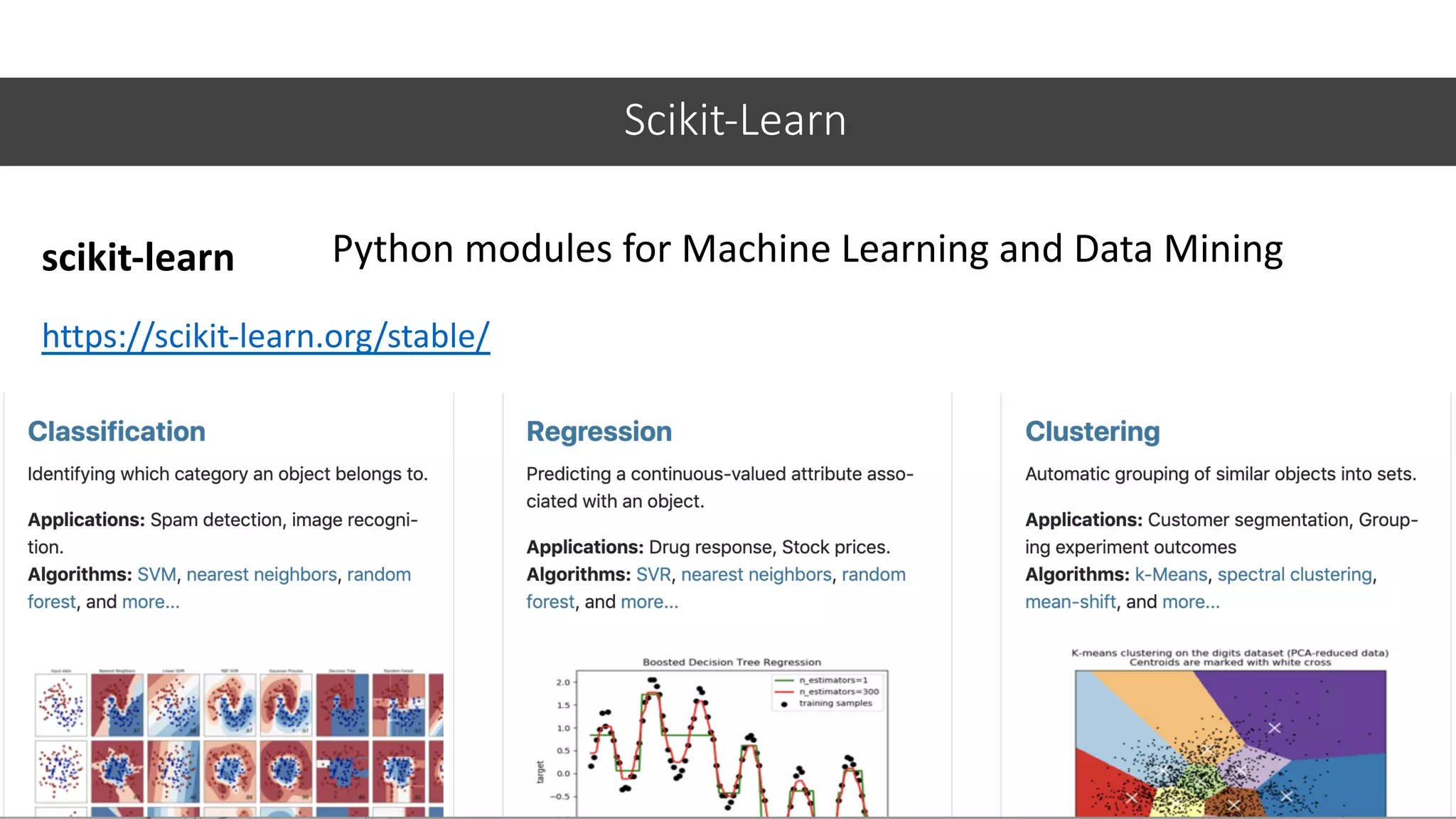
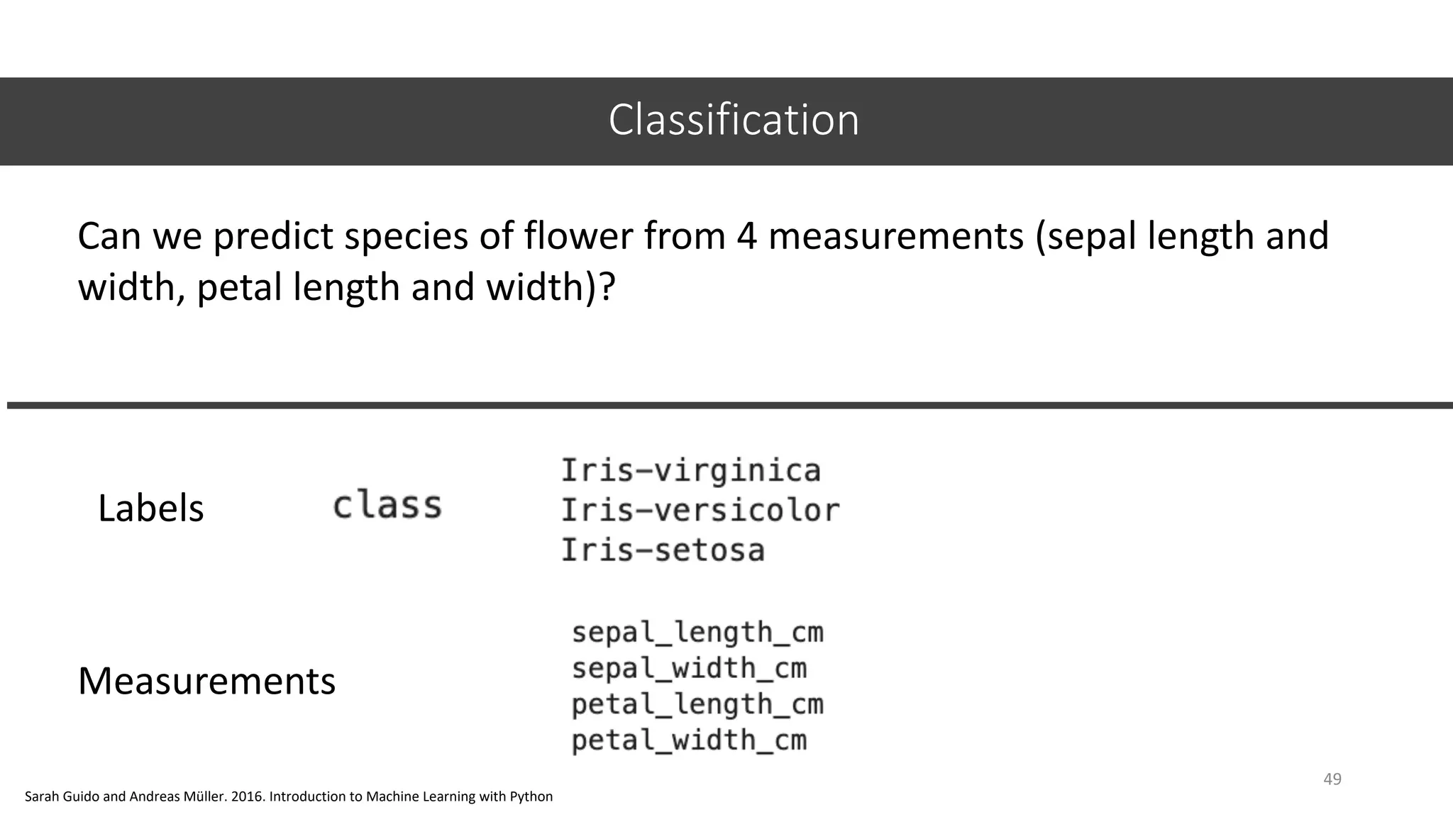
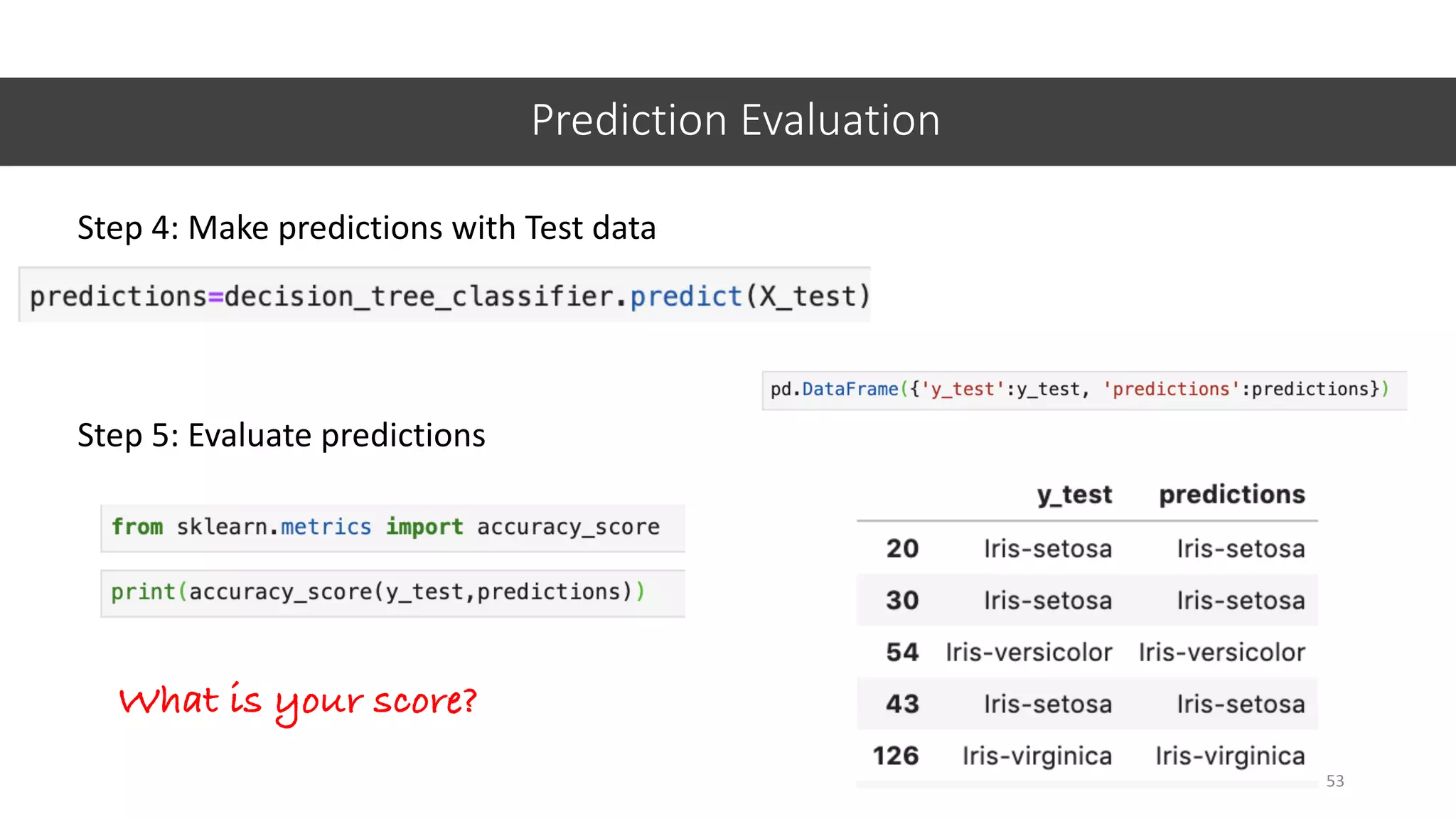
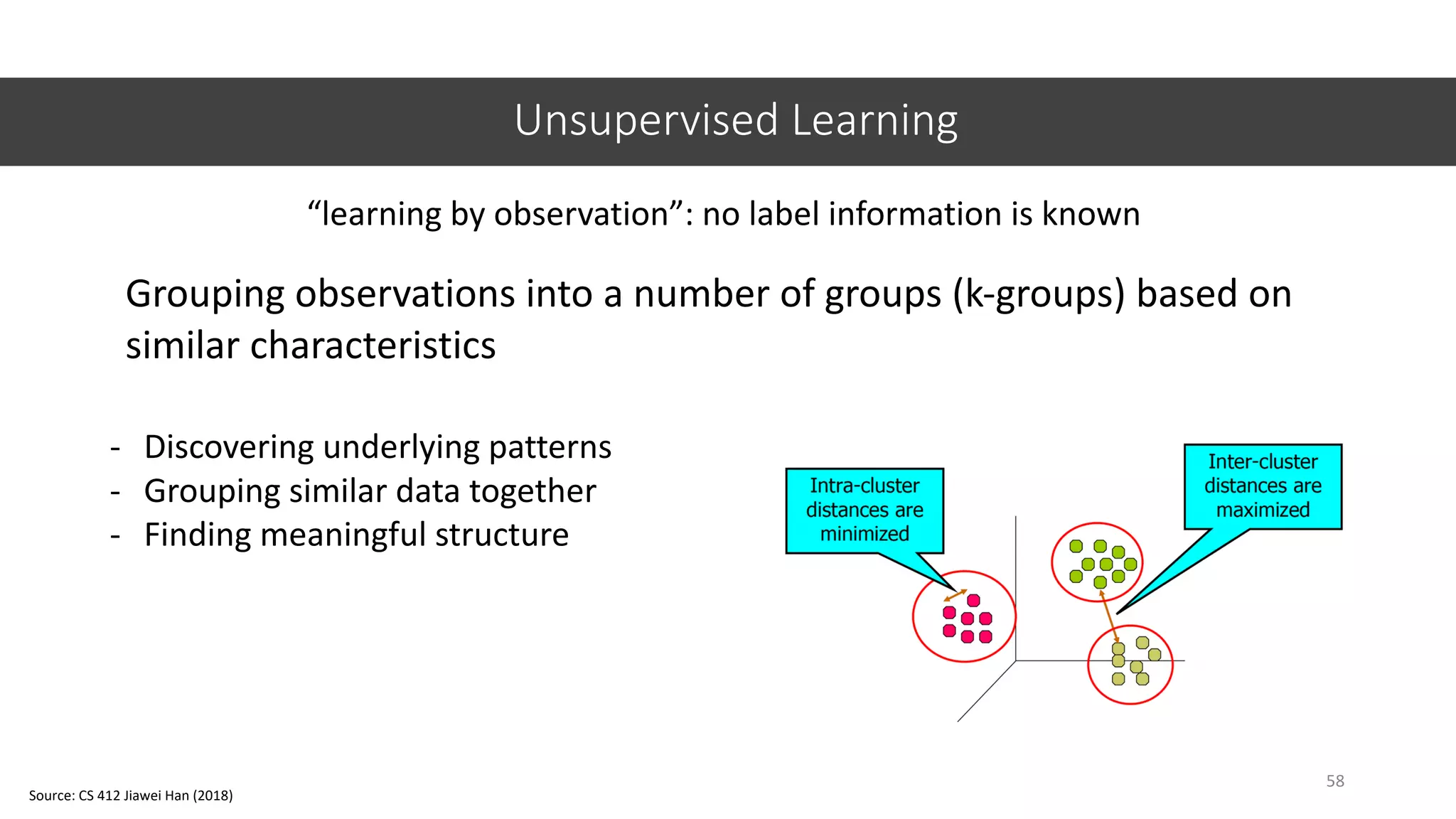
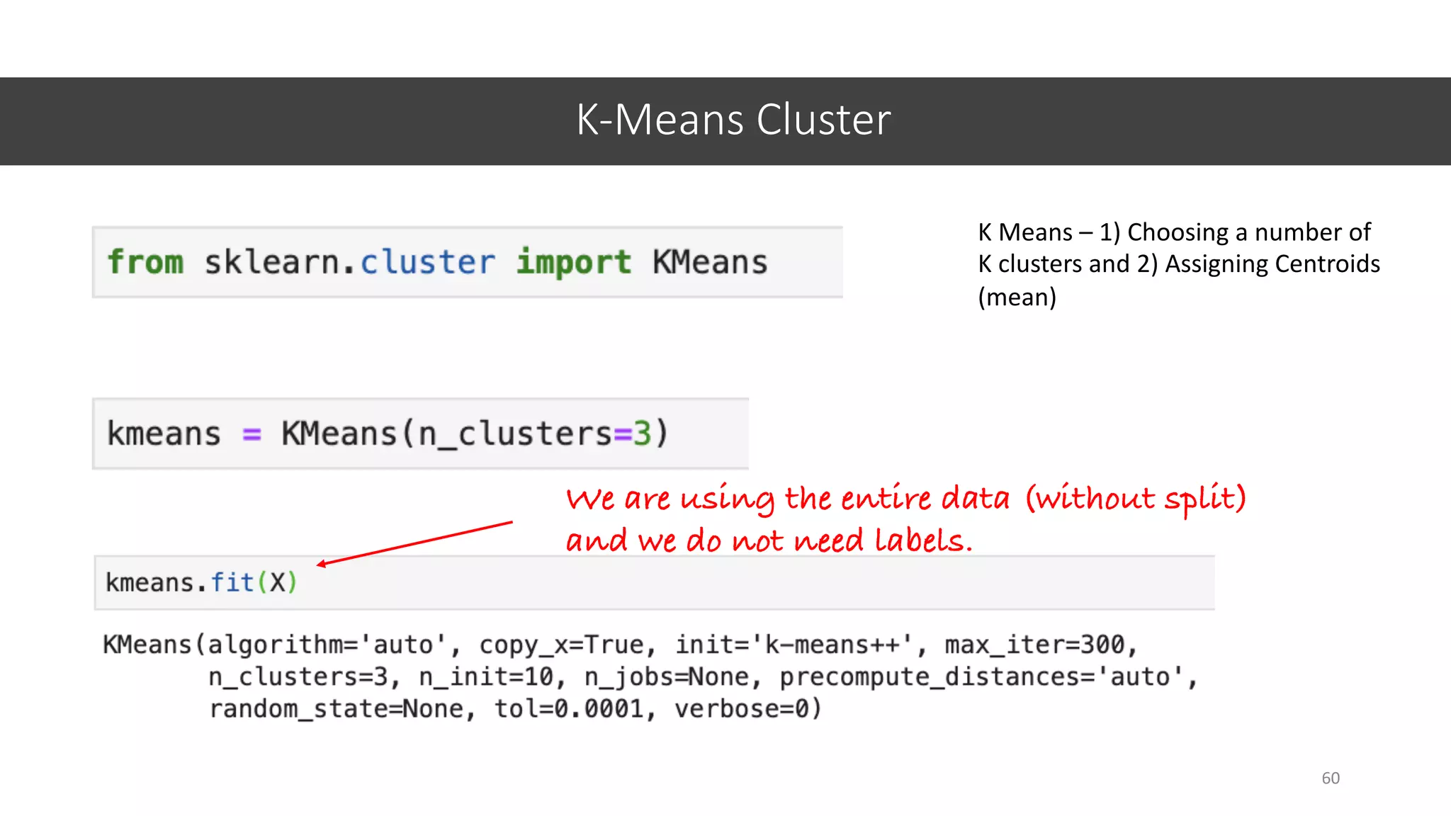
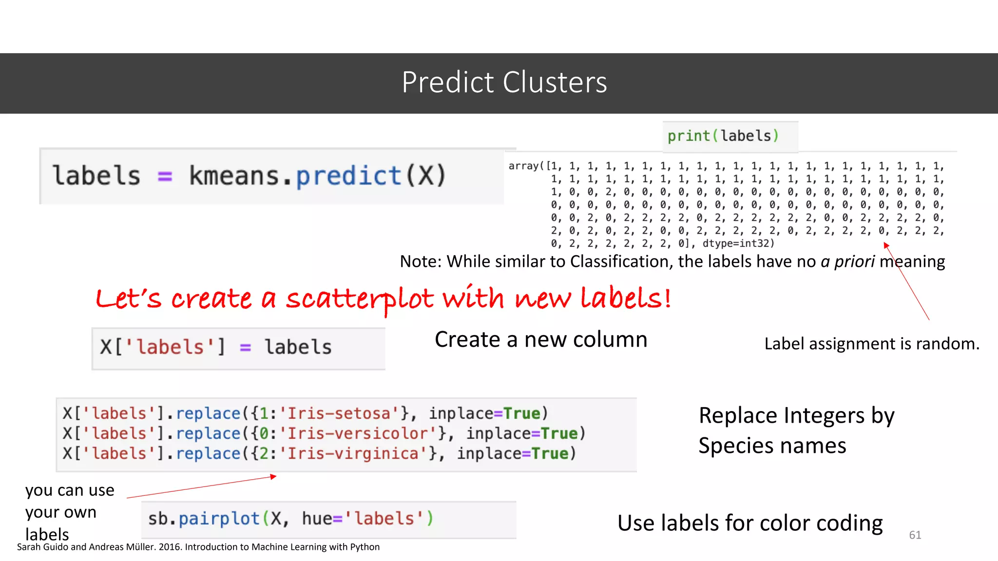
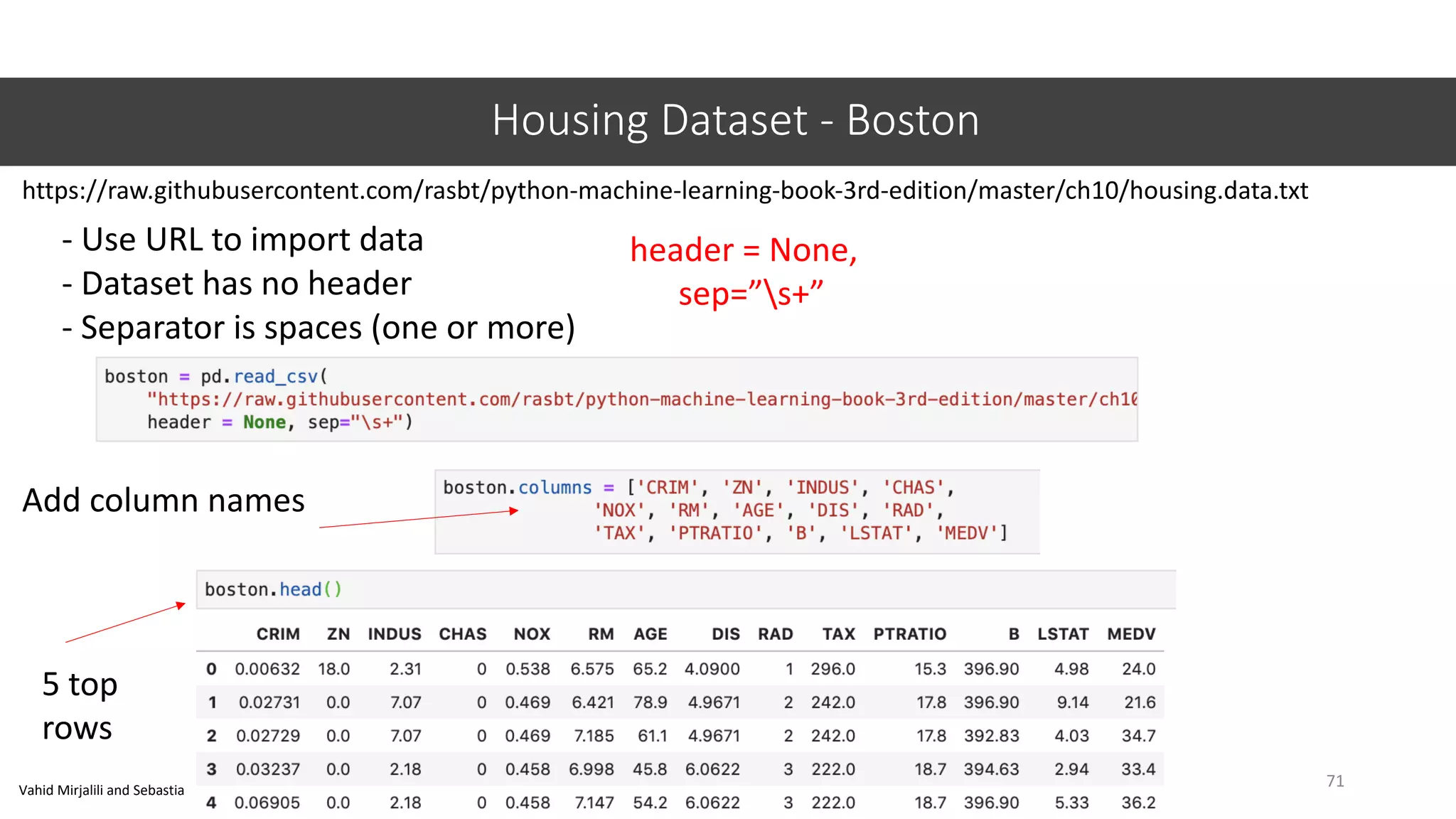
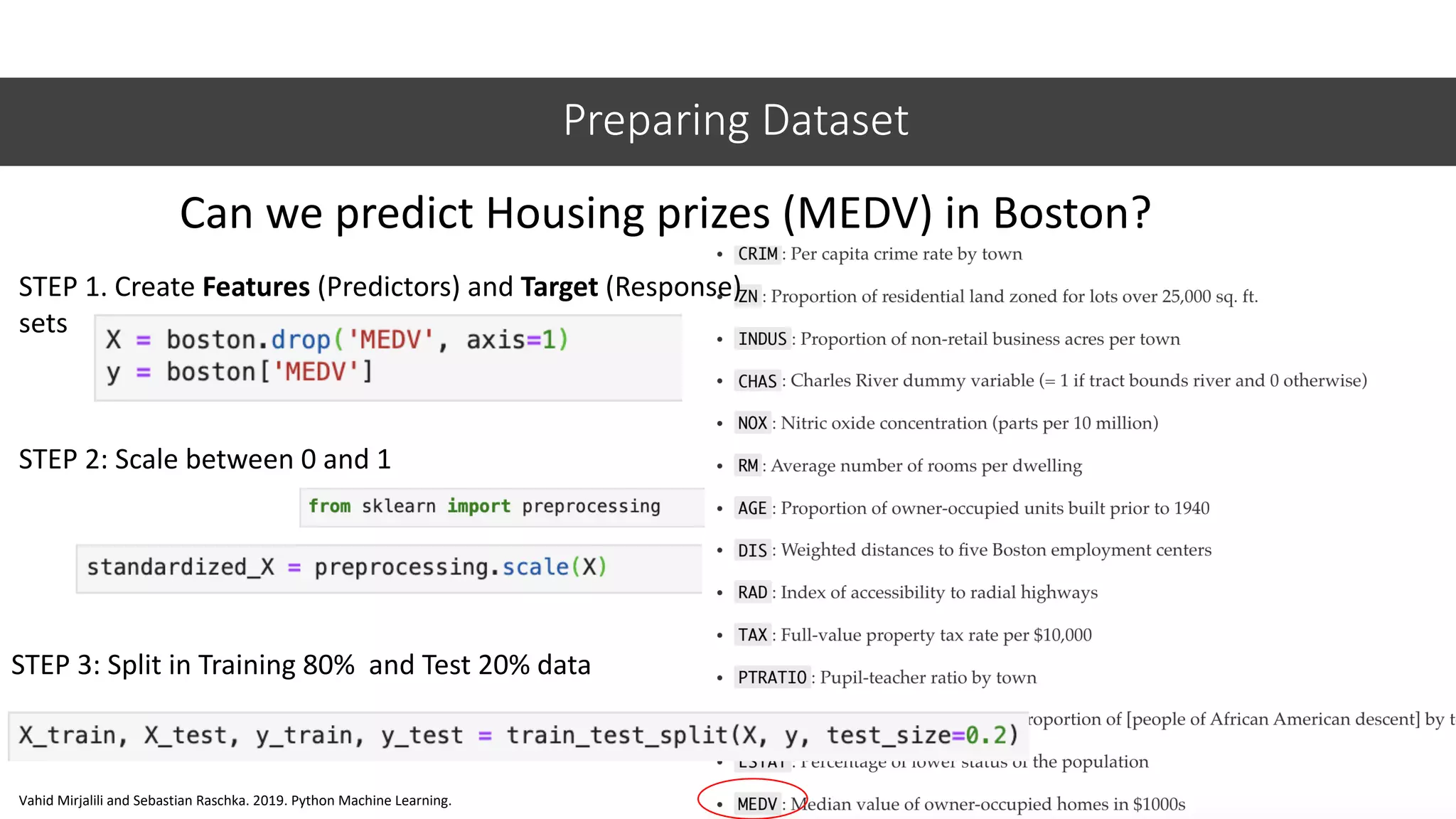
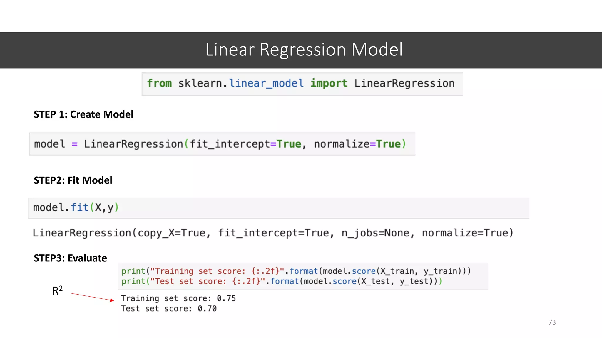
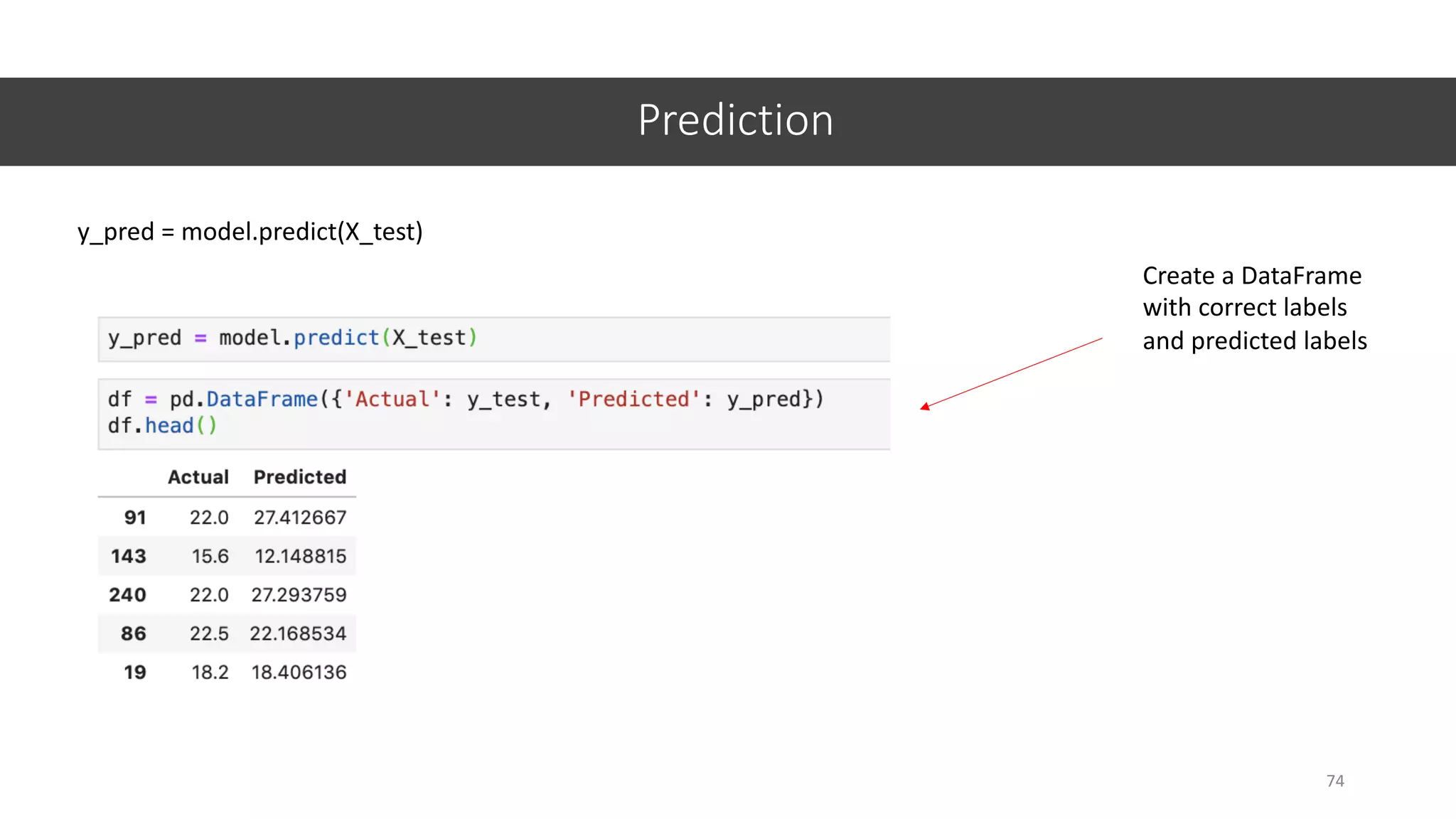
This document provides an overview of machine learning concepts including classification, regression, and clustering. It introduces Jupyter Notebook and shows how to import datasets, clean data, visualize data, train models, and evaluate predictions. Examples use the iris dataset to demonstrate classification with decision trees and k-means clustering. Requirements for linear regression are also outlined. Key Python libraries discussed include pandas, NumPy, matplotlib, and scikit-learn.