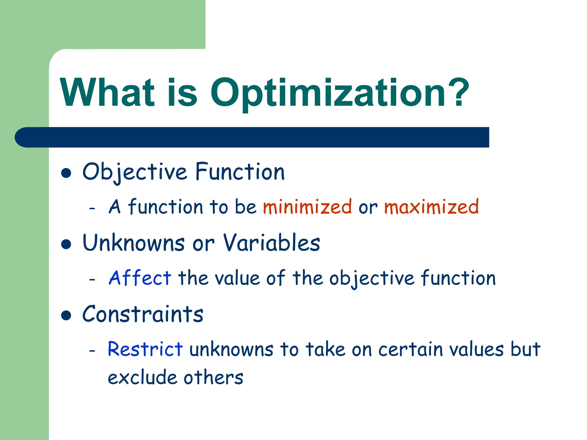
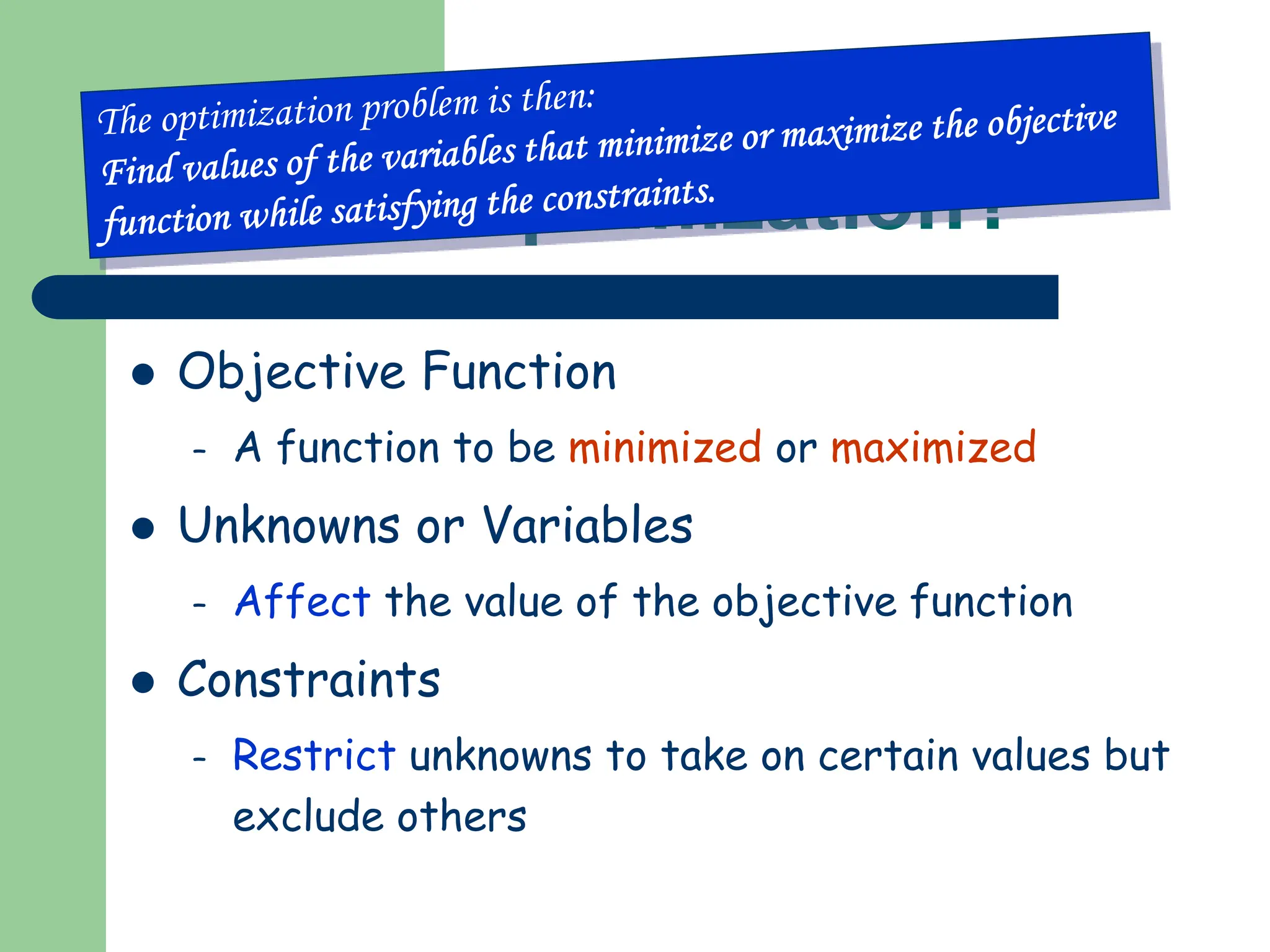
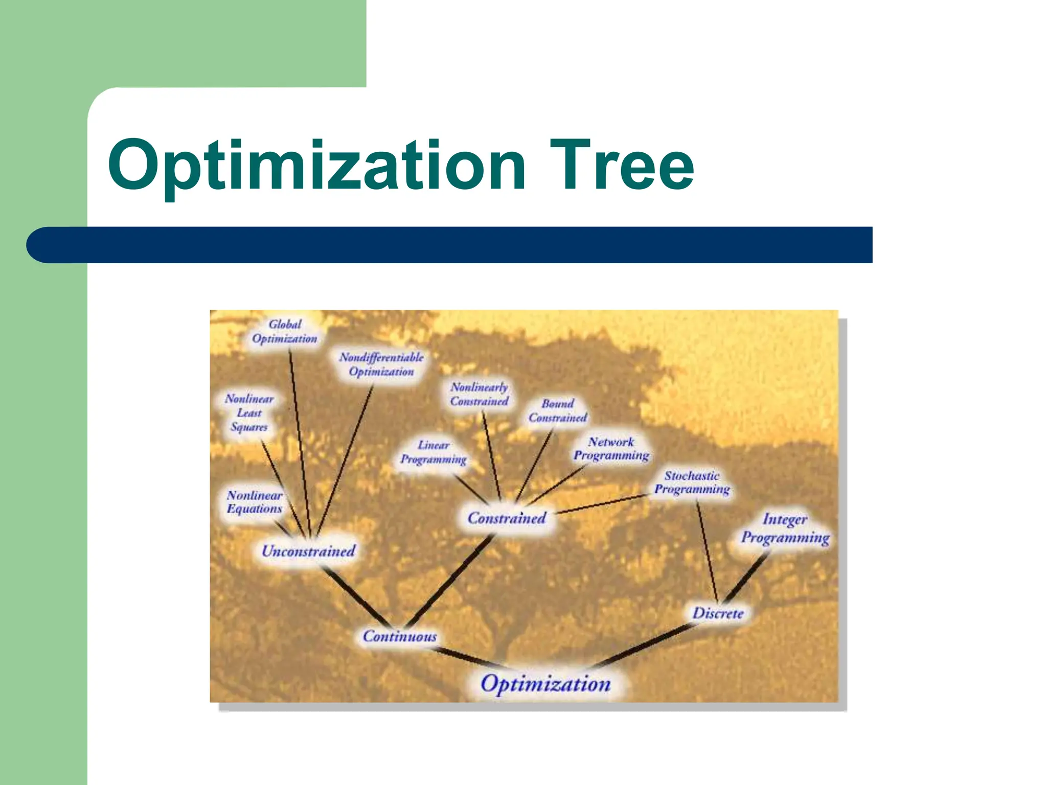
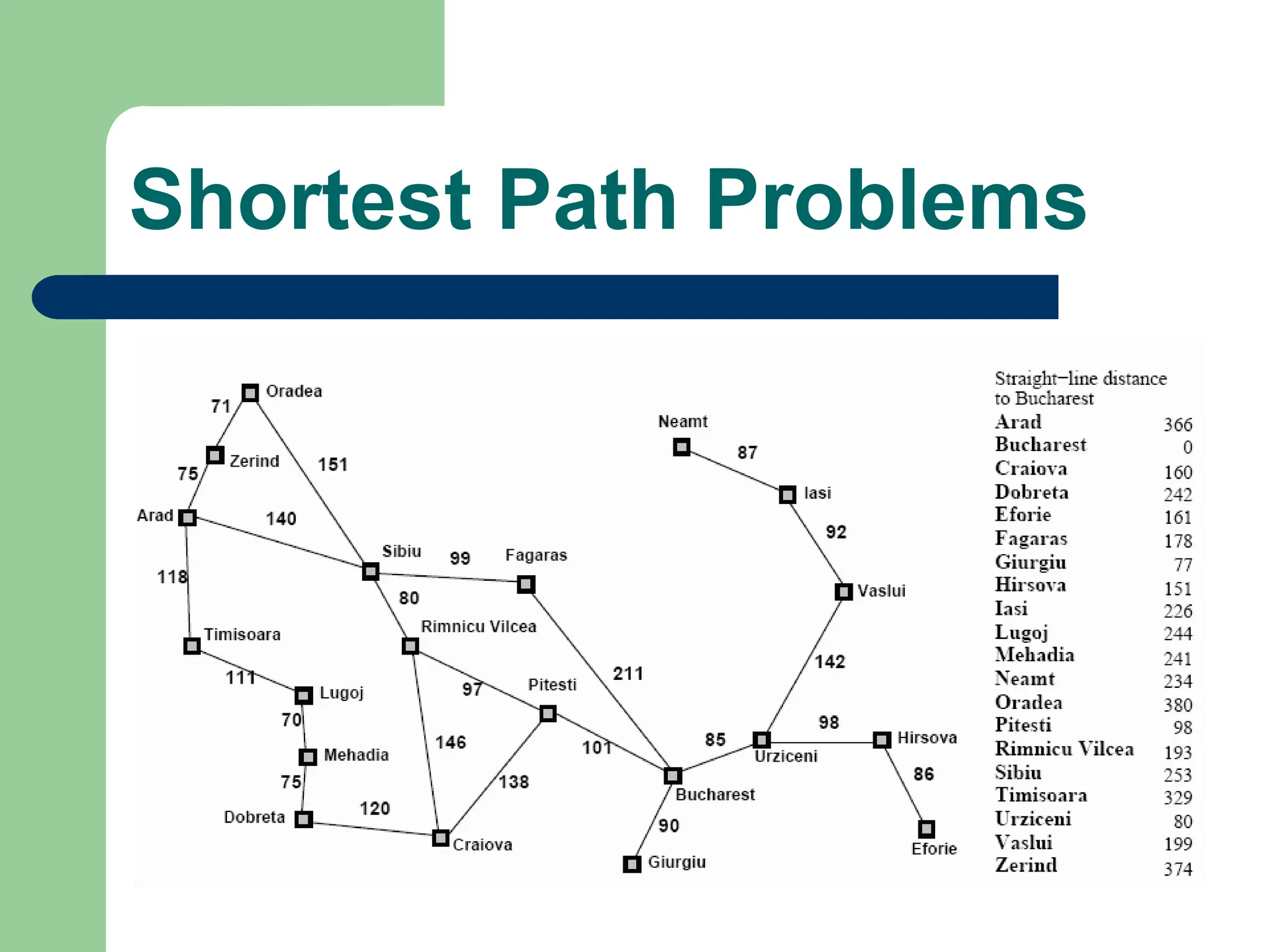
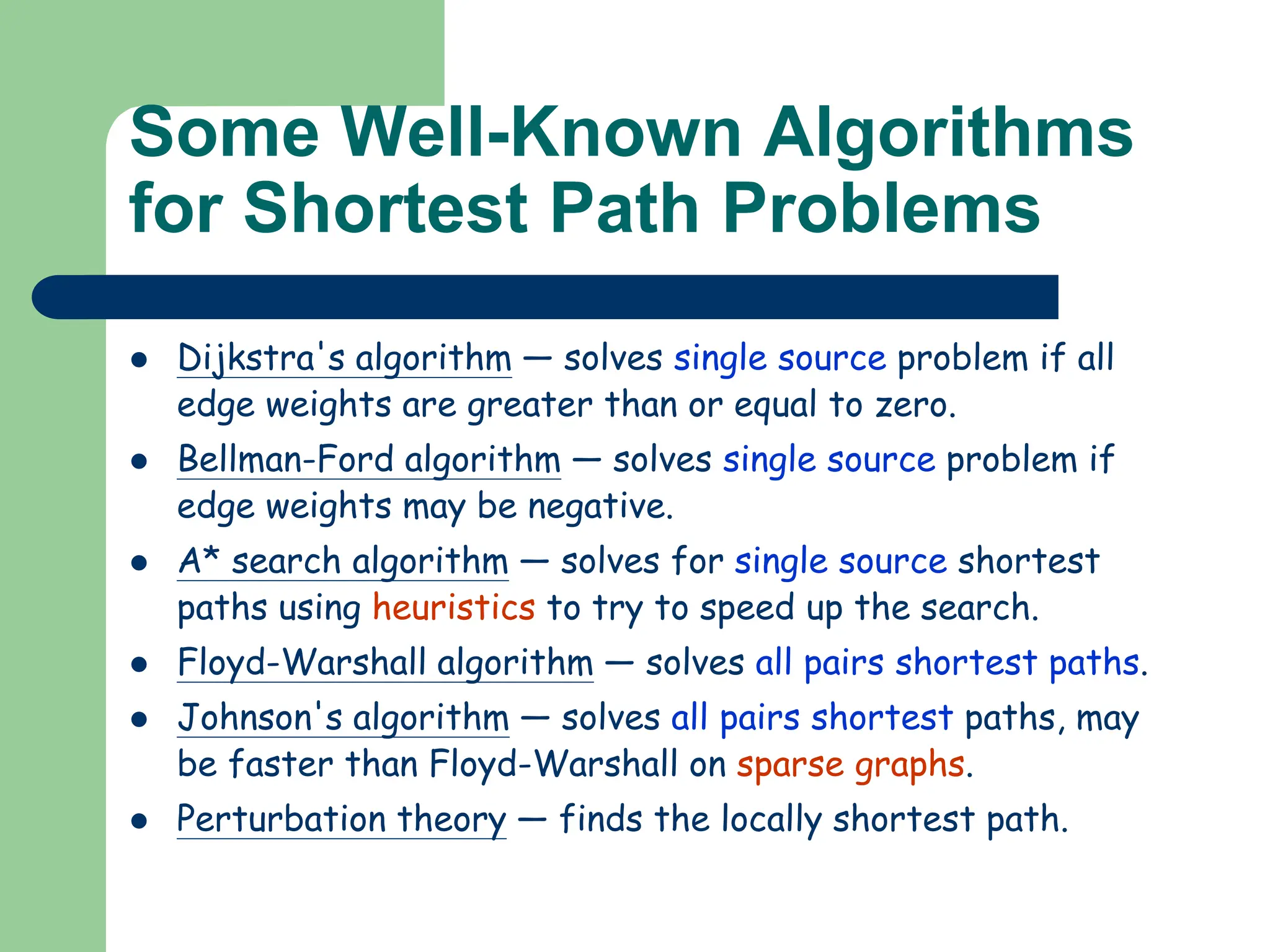
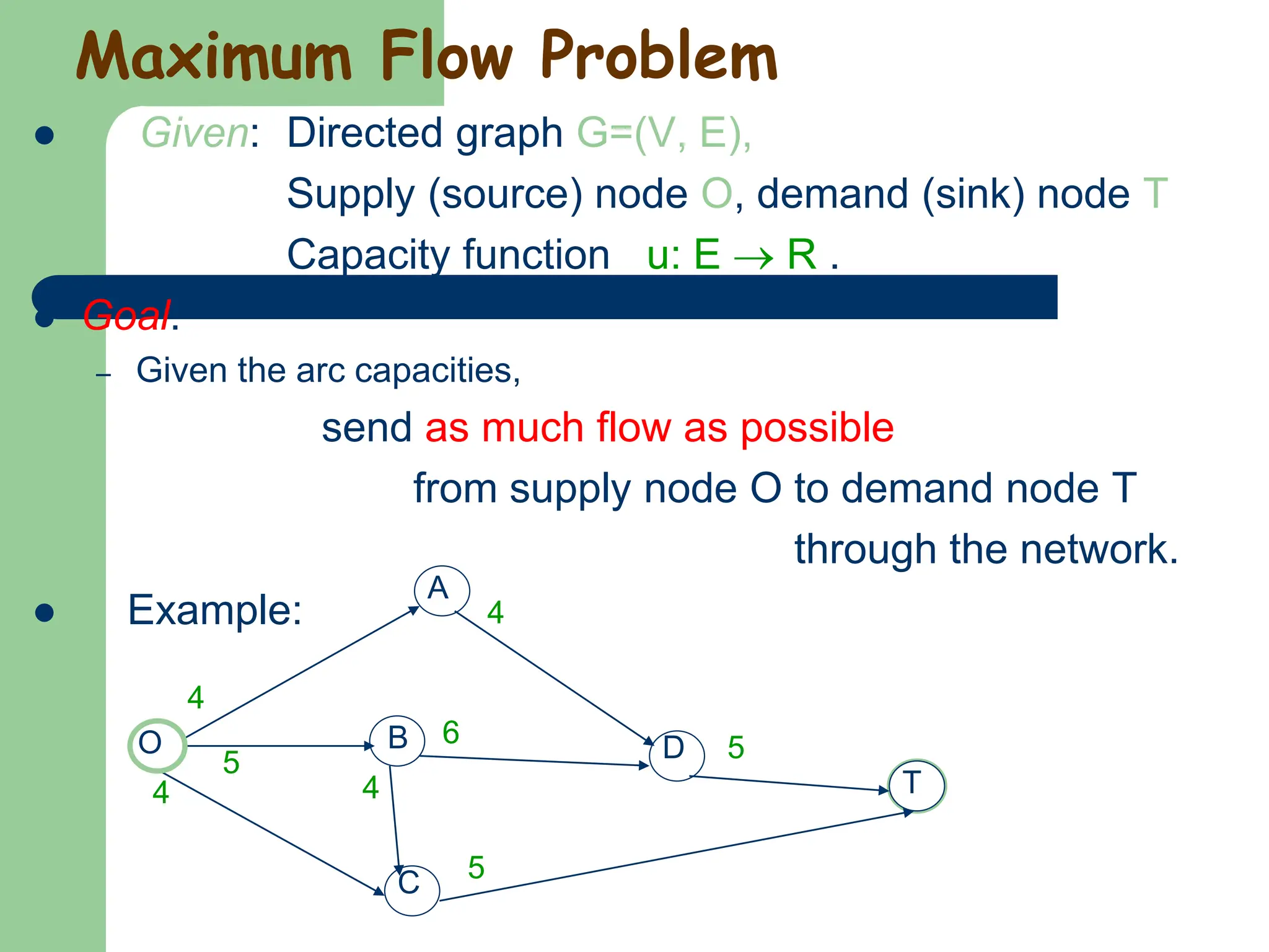
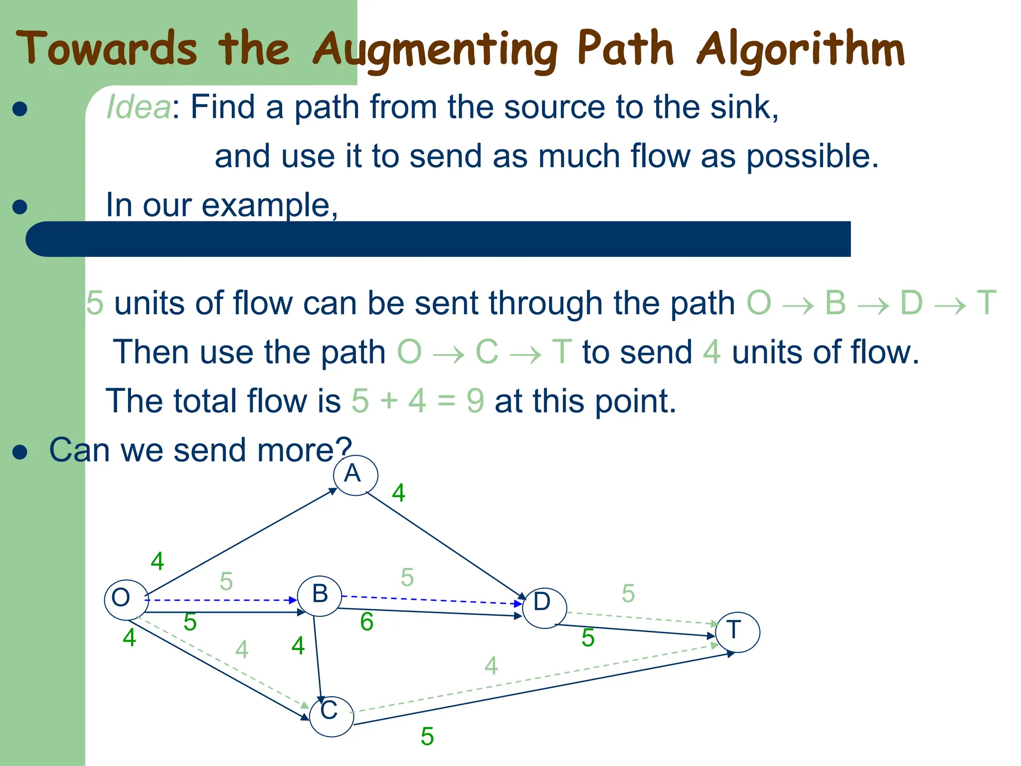
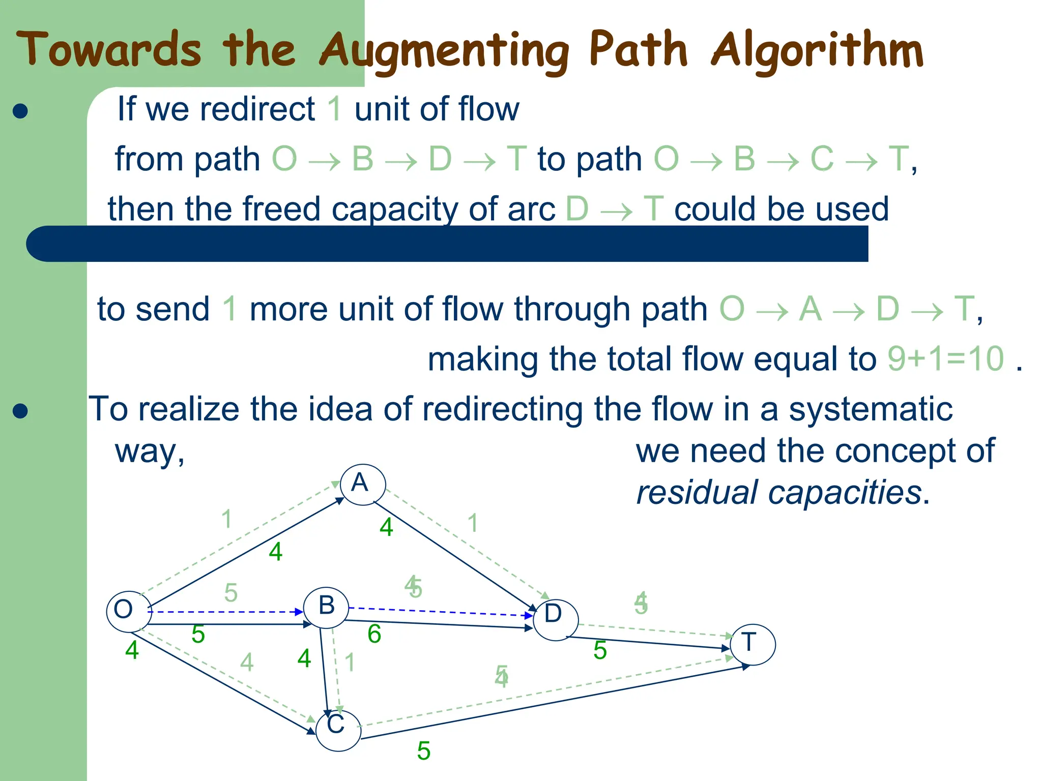
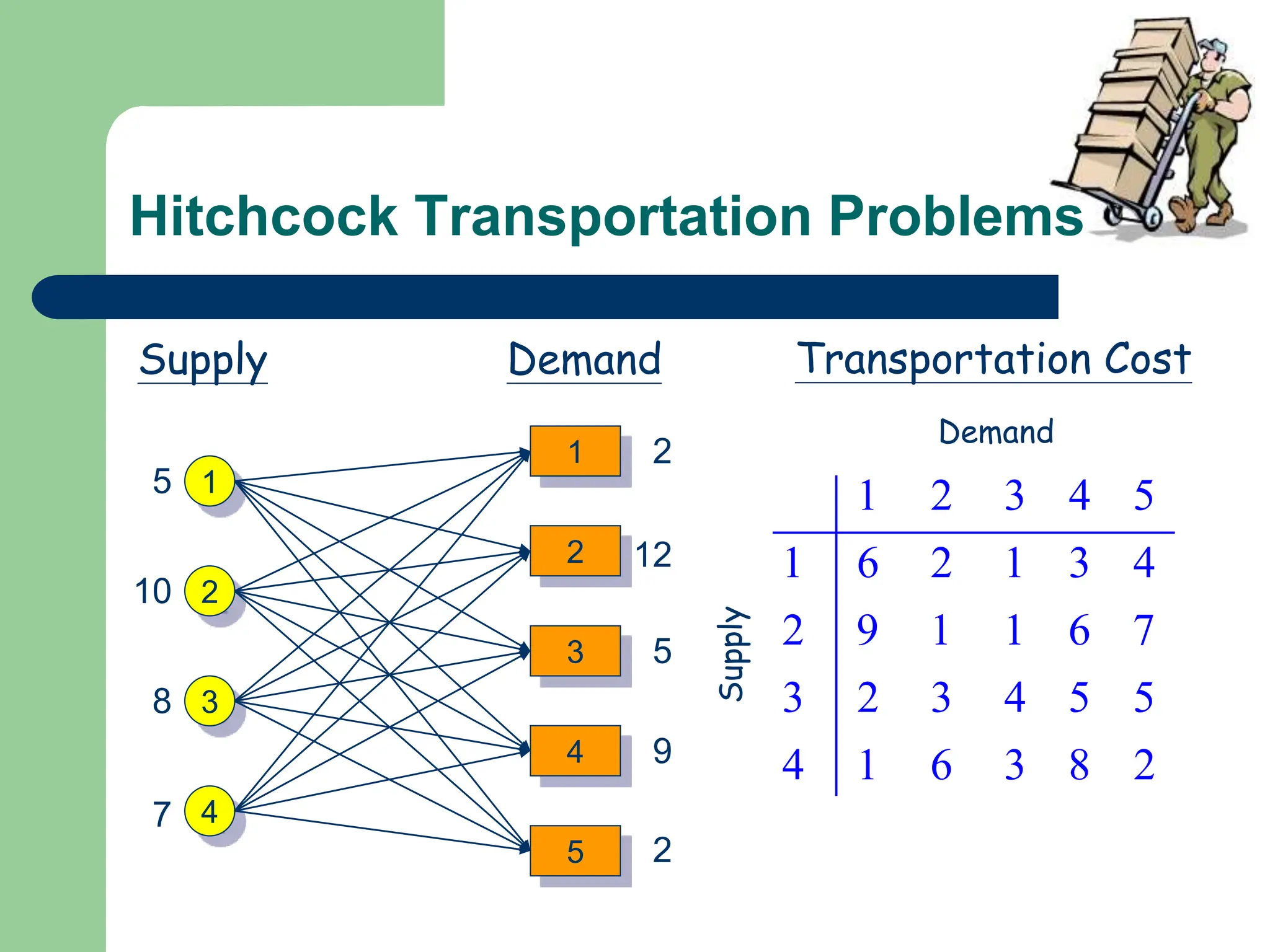
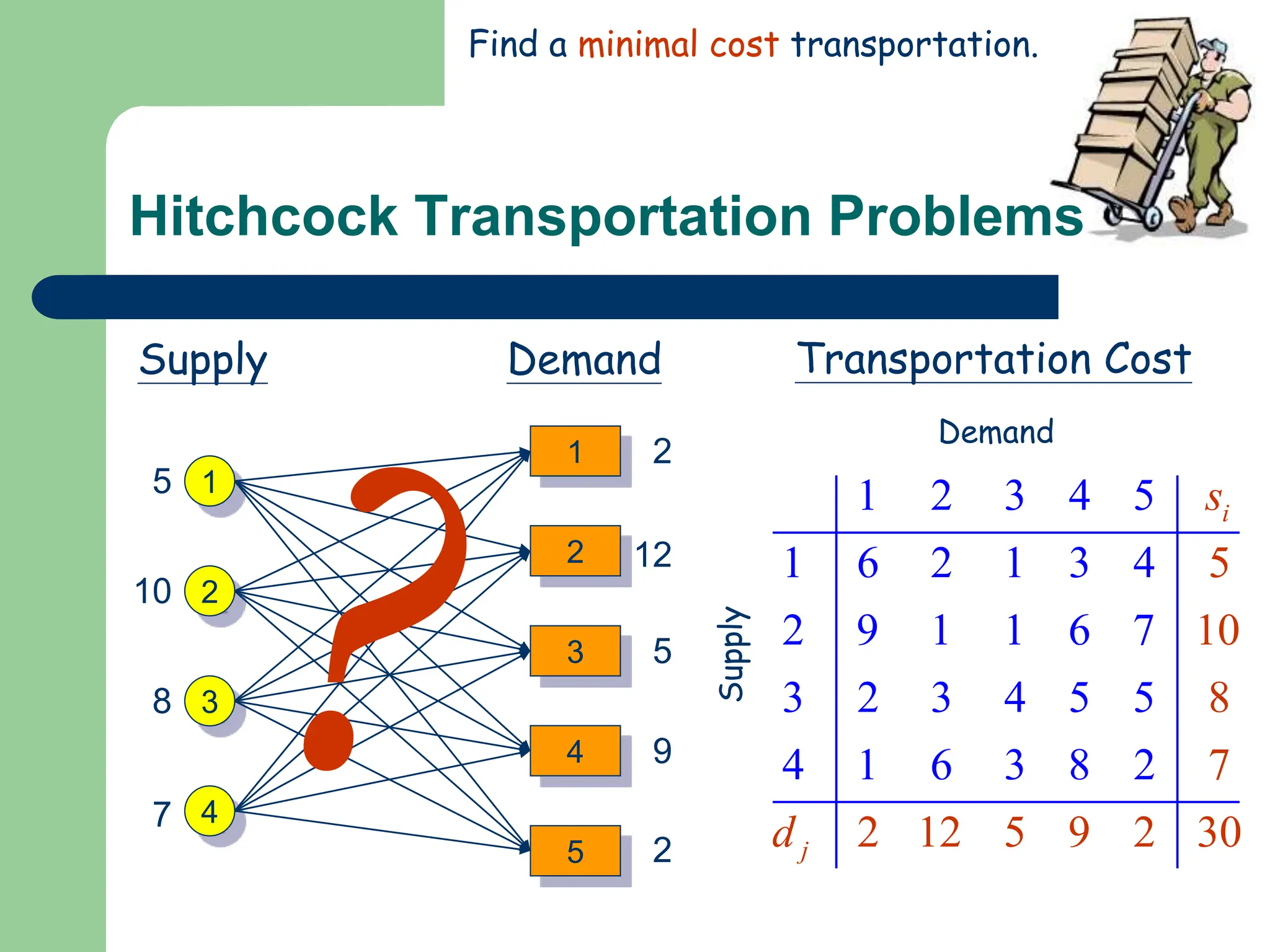
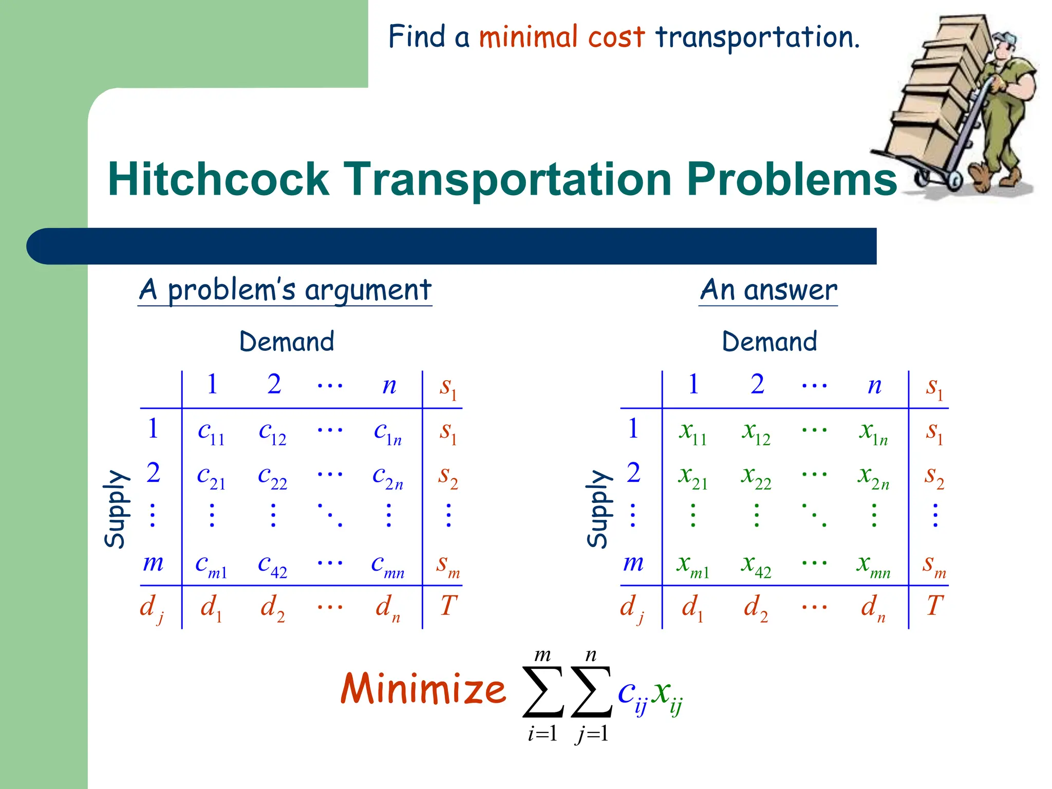
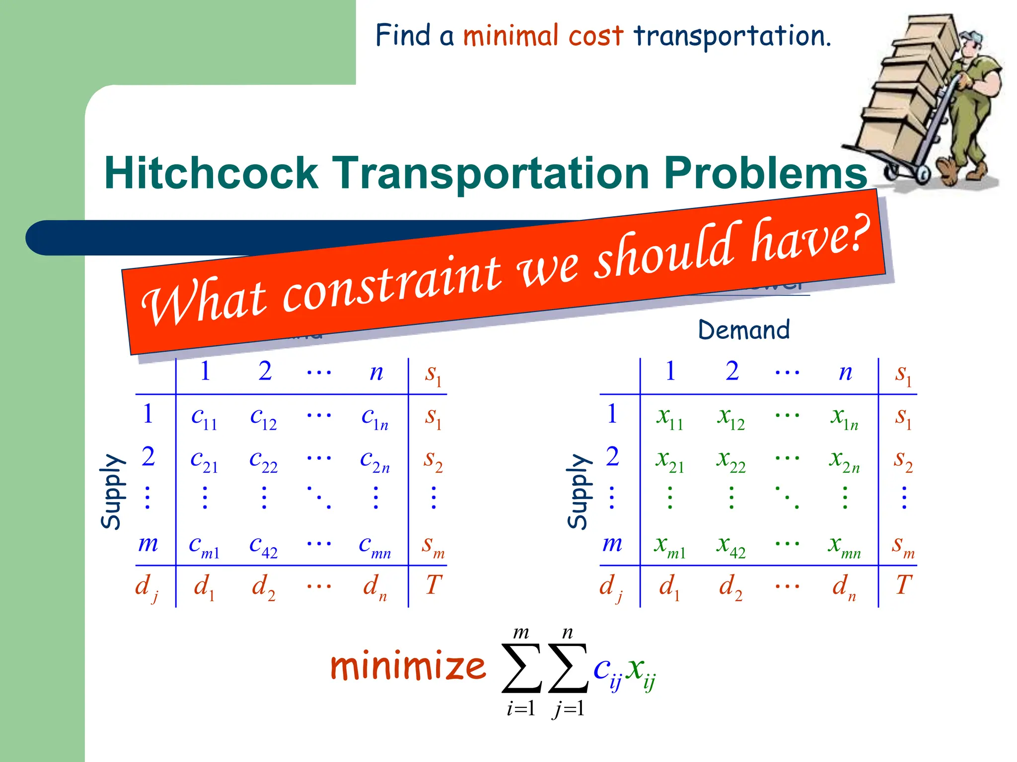
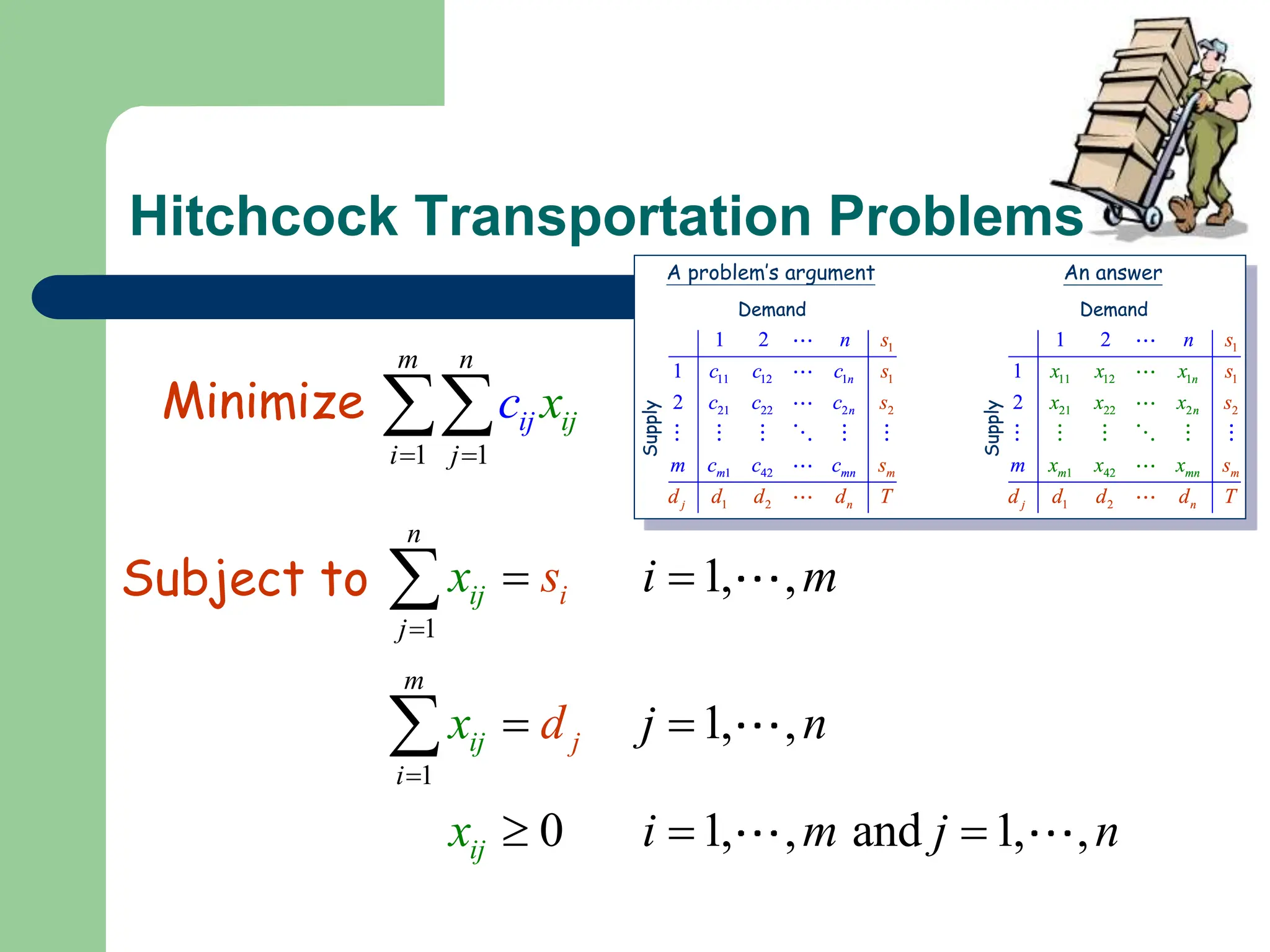
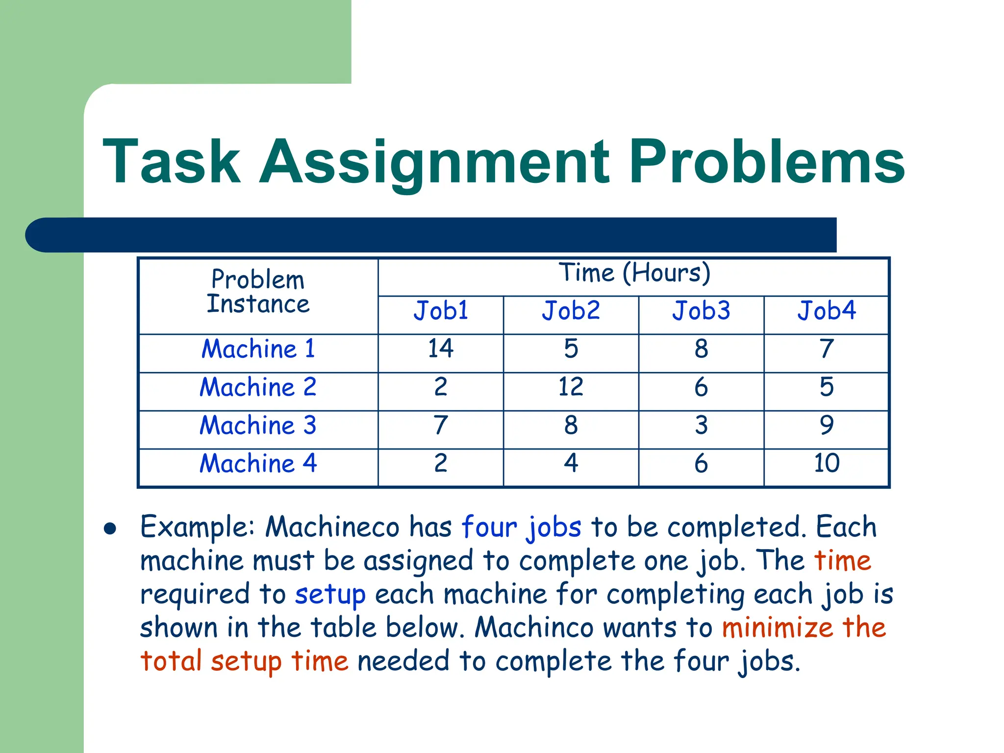
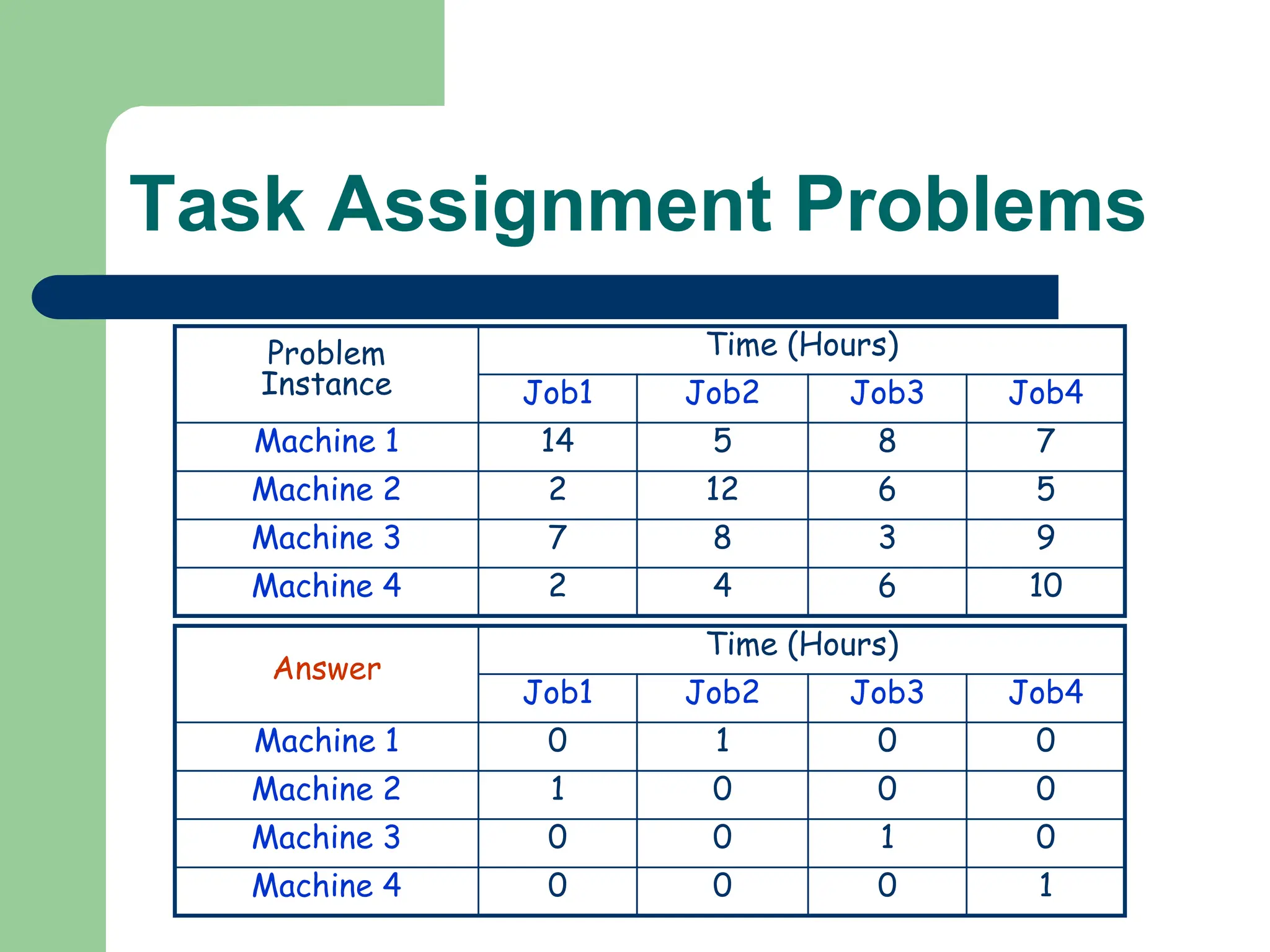
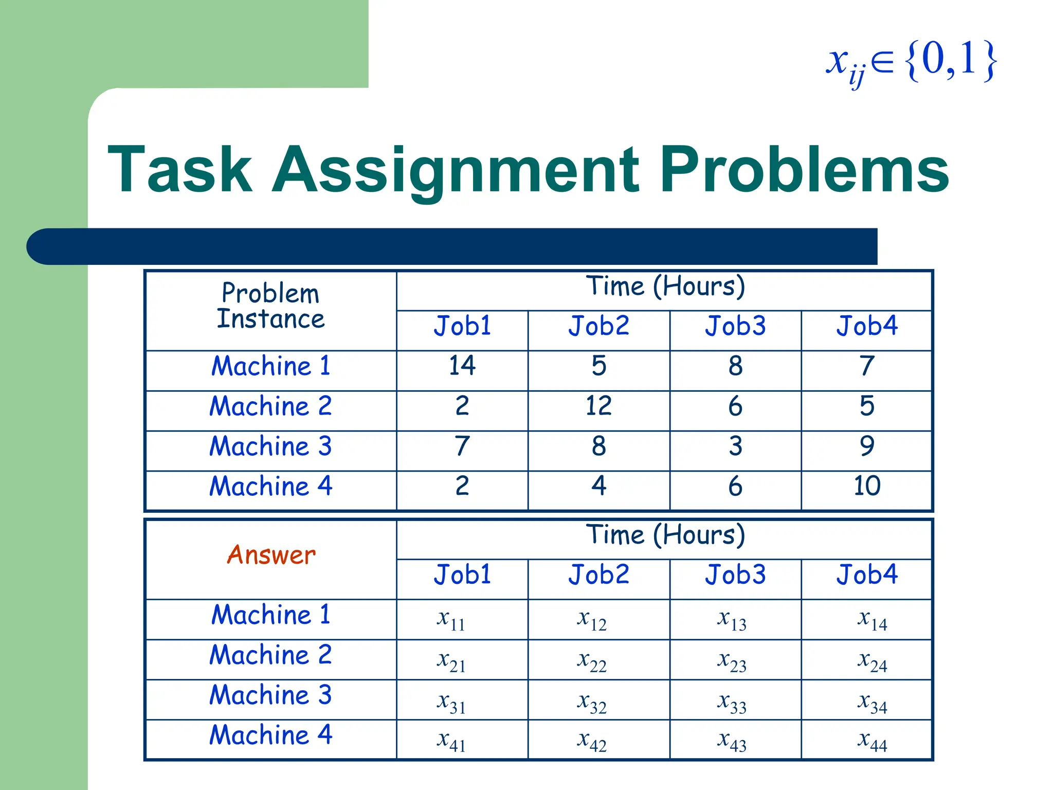
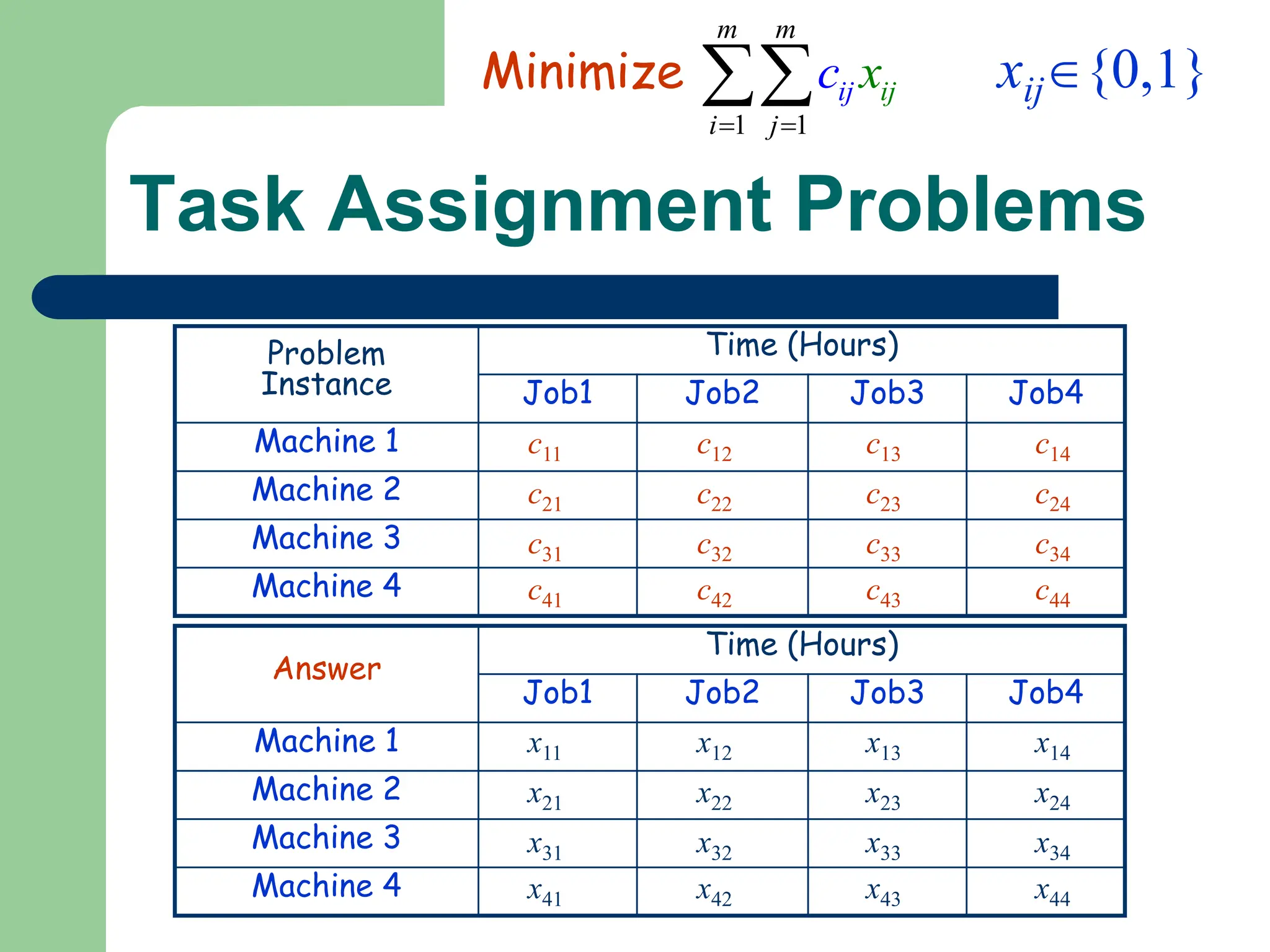
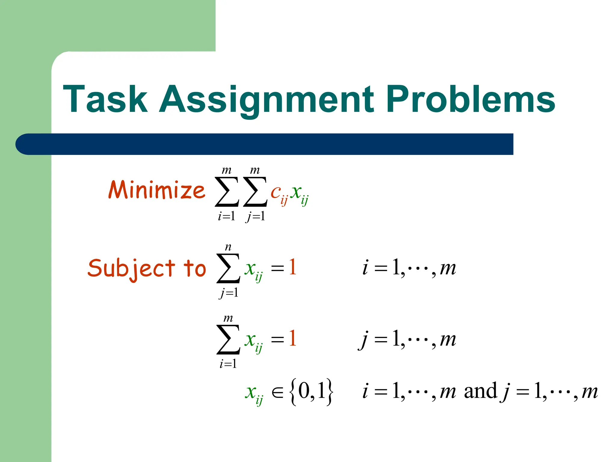
Introduction to Optimization revised.ppt

Lecture 1:
Introduction to the Course of
Optimization
What is
Optimization?

Content
 What is Optimization?
 Categorization of Optimization Problems
 Some Optimization Problems

What is Optimization?
 Objective Function
– A function to be minimized or maximized
 Unknowns or Variables
– Affect the value of the objective function
 Constraints
– Restrict unknowns to take on certain values but
exclude others

Example:
0-1 Knapsack Problem
Which boxes should be chosen
to maximize the amount of
money while still keeping the
overall weight under 15 kg ?

Example:
1 {0,1}
x 
2 {0,1}
x 
3 {0,1}
x 
5 {0,1}
x 
4 {0,1}
x 
 Constraints
's, 1, ,5
i
x i 
 , ,
0,1 1, 5
i
x i
 
1 2 3 4 5
4 2 10 2 1
Maximize
x x x x x
   
1 2 3 4 5
12 1
Subject t
15
4 2
o
1
x x x x x
  
 

Example:
1 2 3 4 5
4 2 10 2
Maxim 1
ize x x x x x
   
 
1 2 3 4 5
12 1 4 2
Subject to 15,
0,1 , 1, ,5
1
i
x x x x x
x i
    
 

Lecture 1:
Optimization
Categorization of
Optimization Problems

Minimum and maximum value of a
function
 This denotes the minimum value of the
objective function , when choosing x from
the set of real numbers . The minimum value
in this case is 1, occurring at x=0 .

Maximum value of a function
 Similarly, the notation
asks for the maximum value of the objective
function 2x, where x may be any real
number. In this case, there is no such
maximum as the objective function is
unbounded, so the answer is "infinity" or
"undefined".

 By convention, the standard form of an optimization
problem is stated in terms of minimization.
 Generally, unless both the objective function and the
feasible region are convex in a minimization
problem, there may be several local minima, where
a local minimum x* is defined as a point for which
there exists some δ > 0 so that for all x such that
 the expression
 holds; that is to say, on some region around x* all of
the function values are greater than or equal to the
value at that point. Local maxima are defined
similarly.

Ingredients of Optimization Problems
 Constraints

Optimization Problems w/o
Objective Function
 In some cases, the goal is to find a set of
variables that satisfies some constraints only, e.g.,
– circuit layouts
– n-queen
– Sudoku
 This type of problems is usually called a
feasibility problem or constraint satisfaction
problem.
• Objective Function
• Unknowns or Variables
• Constraints

Optimization Problems w/
Multiple Objective Functions
 Sometimes, we need to optimize a number of different
objectives at once, e.g.,
– In the panel design problem, it would be nice to minimize
weight and maximize strength simultaneously.
 Usually, the different objectives are not compatible
– The variables that optimize one objective may be far from
optimal for the others.
 In practice, problems with multiple objectives are
reformulated as single-objective problems by either
forming a weighted combination of the different objectives
or else replacing some of the objectives by constraints.
• Constraints

Variables
• Constraints
 Variables are essential.
– Without variables, we cannot define the objective
function and the problem constraints.
 Continuous Optimization
– all the variables are allowed to take values from
subintervals of the real line;
 Discrete Optimization
– require some or all of the variables to have integer values.

Constraints
• Constraints
 Constraints are not essential.
 Unconstrained optimization
– A large and important one for which a lot of algorithms
and software are available.
 However, almost all problems really do have
constraints, e.g.,
– Any variable denoting the “number of objects” in a system
can only be useful if it is less than the number of
elementary particles in the known universe!
– In practice, though, answers that make good sense in
terms of the underlying physical or economic problem can
often be obtained without putting constraints on the
variables.

Lecture 1:
Optimization
Some
Optimization Problems

Some Well-Known Algorithms
for Shortest Path Problems
 Dijkstra's algorithm — solves single source problem if all
edge weights are greater than or equal to zero.
 Bellman-Ford algorithm — solves single source problem if
edge weights may be negative.
 A* search algorithm — solves for single source shortest
paths using heuristics to try to speed up the search.
 Floyd-Warshall algorithm — solves all pairs shortest paths.
 Johnson's algorithm — solves all pairs shortest paths, may
be faster than Floyd-Warshall on sparse graphs.
 Perturbation theory — finds the locally shortest path.

Maximum Flow Problem
 Given: Directed graph G=(V, E),
Supply (source) node O, demand (sink) node T
Capacity function u: E  R .
 Goal:
– Given the arc capacities,
send as much flow as possible
from supply node O to demand node T
through the network.
 Example:
4
4
5
6
4
4
5
5
O
A
D
B
C
T

Towards the Augmenting Path Algorithm
 Idea: Find a path from the source to the sink,
and use it to send as much flow as possible.
 In our example,
5 units of flow can be sent through the path O  B  D  T
Then use the path O  C  T to send 4 units of flow.
The total flow is 5 + 4 = 9 at this point.
 Can we send more?
O
A
D
B
C
T
4
4
5 6
4
4 5
5
5 5
4
4
5

Towards the Augmenting Path Algorithm
 If we redirect 1 unit of flow
from path O  B  D  T to path O  B  C  T,
then the freed capacity of arc D  T could be used
to send 1 more unit of flow through path O  A  D  T,
making the total flow equal to 9+1=10 .
 To realize the idea of redirecting the flow in a systematic
way, we need the concept of
residual capacities.
O
A
D
B
C
T
4
4
5 6
4
4 5
5
5 5
5
4
4
4
4
1 5
1 1

Hitchcock Transportation Problems
Supply Demand
1
2
3
4
1
2
3
4
5
5
10
8
7
2
12
5
9
2
1 2 3 4 5
1 6 2 1 3 4
2 9 1 1 6 7
3 2 3 4 5 5
4 1 6 3
5
10
8
7
2 12 5 9 2
8
30
2
i
j
s
d
Demand
Supply
Transportation Cost

Supply Demand
1
2
3
4
1
2
3
4
5
5
10
8
7
2
12
5
9
2
1 2 3 4 5
1 6 2 1 3 4
2 9 1 1 6 7
3 2 3 4 5 5
4 1 6 3
5
10
8
7
2 12 5 9 2
8
30
2
i
j
s
d
Demand
Supply
Transportation Cost
Find a minimal cost transportation.

A problem’s argument
11 12 1
21 22 2
1
1
1
2
1
4
2
2
1 2
1
2
n
m
n
m mn
j
n
s
s
s
n
c c c
c
s
d d d d
c c
c c c
T
m
Supply
Demand
11 12 1
21 22 2
1
1
1
2
1
4
2
2
1 2
1
2
n
m
n
m mn
j
n
s
s
s
x x x
x
s
x
d d d
x
T
x
x x
d
n
m
Supply
Demand
An answer
1 1
m n
i j
j
j i
i x
c
 

Minimize

11 12 1
21 22 2
1
1
1
2
1
4
2
2
1 2
1
2
n
m
n
m mn
j
n
s
s
s
n
c c c
c
s
d d d d
c c
c c c
T
m
Supply
Demand
11 12 1
21 22 2
1
1
1
2
1
4
2
2
1 2
1
2
n
m
n
m mn
j
n
s
s
s
x x x
x
s
x
d d d
x
T
x
x x
d
n
m
Supply
Demand
An answer
1 1
m n
i j
j
j i
i x
c
 

minimize

1 1
m n
i j
j
j i
i x
c
 

Minimize
1
1
1, ,
1, ,
0 1, , and 1, ,
i
j
n
j
m
i
ij
ij
ij
i m
j n
i m j n
s
x
x
x
d


 
 
  


Subject to
11 12 1
21 22 2
1
1
1
2
1
4
2
2
1 2
1
2
n
m
n
m mn
j
n
s
s
s
n
c c c
c
s
d d d d
c c
c c c
T
m
Supply
Demand
11 12 1
21 22 2
1
1
1
2
1
4
2
2
1 2
1
2
n
m
n
m mn
j
n
s
s
s
n
c c c
c
s
d d d d
c c
c c c
T
m
Supply
Demand
11 12 1
21 22 2
1
1
1
2
1
4
2
2
1 2
1
2
n
m
n
m mn
j
n
s
s
s
x x x
x
s
x
d d d
x
T
x
x x
d
n
m
Supply
Demand
11 12 1
21 22 2
1
1
1
2
1
4
2
2
1 2
1
2
n
m
n
m mn
j
n
s
s
s
x x x
x
s
x
d d d
x
T
x
x x
d
n
m
Supply
Demand
An answer

Task Assignment Problems
 Example: Machineco has four jobs to be completed. Each
machine must be assigned to complete one job. The time
required to setup each machine for completing each job is
shown in the table below. Machinco wants to minimize the
total setup time needed to complete the four jobs.
Problem
Instance
Time (Hours)
Job1 Job2 Job3 Job4
Machine 1 14 5 8 7
Machine 2 2 12 6 5
Machine 3 7 8 3 9
Machine 4 2 4 6 10

Problem
Instance
Time (Hours)
Job1 Job2 Job3 Job4
Machine 1 14 5 8 7
Machine 2 2 12 6 5
Machine 3 7 8 3 9
Machine 4 2 4 6 10
Answer
Time (Hours)
Job1 Job2 Job3 Job4
Machine 1 0 1 0 0
Machine 2 1 0 0 0
Machine 3 0 0 1 0
Machine 4 0 0 0 1

Answer
Time (Hours)
Job1 Job2 Job3 Job4
Machine 1 0 1 0 0
Machine 2 1 0 0 0
Machine 3 0 0 1 0
Machine 4 0 0 0 1
Problem
Instance
Time (Hours)
Job1 Job2 Job3 Job4
Machine 1 14 5 8 7
Machine 2 2 12 6 5
Machine 3 7 8 3 9
Machine 4 2 4 6 10
Answer
Time (Hours)
Job1 Job2 Job3 Job4
Machine 1
Machine 2
Machine 3
Machine 4
x11 x12 x13 x14
x21 x22 x23 x24
x31 x32 x33 x34
x41 x42 x43 x44
xij{0,1}

Answer
Time (Hours)
Job1 Job2 Job3 Job4
Machine 1 0 1 0 0
Machine 2 1 0 0 0
Machine 3 0 0 1 0
Machine 4 0 0 0 1
Problem
Instance
Time (Hours)
Job1 Job2 Job3 Job4
Machine 1 14 5 8 7
Machine 2 2 12 6 5
Machine 3 7 8 3 9
Machine 4 2 4 6 10
Answer
Time (Hours)
Job1 Job2 Job3 Job4
Machine 1
Machine 2
Machine 3
Machine 4
x11 x12 x13 x14
x21 x22 x23 x24
x31 x32 x33 x34
x41 x42 x43 x44
xij{0,1}
Problem
Instance
Time (Hours)
Job1 Job2 Job3 Job4
Machine 1
Machine 2
Machine 3
Machine 4
c11 c12 c13 c14
c21 c22 c23 c24
c31 c32 c33 c34
c41 c42 c43 c44
1 1
m m
i j
j
j i
i x
c
 

Minimize

1 1
m m
i j
j
j i
i x
c
 

Minimize
 
1
1
1, ,
1, ,
0,1 1, , and 1,
1
,
1
ij
i
j
i
j
i
n
j
m
i m
j m
x
i m j
x
m
x


 
 
  


Subject to

Traveling Salesman Problem (TSP)

Traveling Salesman Problem (TSP)
How many feasible paths?
n cities
! ( 1)!
2 2
n n
n



Bin-Packing Problems
 Determine how to put the given objects in
the least number of fixed space bins.
 There are many variants, such as, 3D, 2D,
linear, pack by volume, pack by weight,
minimize volume, maximize value, fixed
shape objects, etc.

Bin-Packing Problems
Example: suppose we need a
number of pipes of different,
specific lengths to plumb a
house and we can buy pipe
stock in 5 meter lengths.
How can we cut the 5 meter
pipes to waste as little as
possible, i.e., to minimize the
cost of pipe?

Introduction to Optimization revised.ppt

More Related Content

What's hot

Similar to Introduction to Optimization revised.ppt

Recently uploaded

Introduction to Optimization revised.ppt